LEARNING SUPER-FEATURES FOR IMAGE RETRIEVAL
←
→
Page content transcription
If your browser does not render page correctly, please read the page content below

Published as a conference paper at ICLR 2022

L EARNING S UPER - FEATURES FOR I MAGE R ETRIEVAL
 Philippe Weinzaepfel, Thomas Lucas, Diane Larlus, and Yannis Kalantidis
 NAVER LABS Europe, Grenoble, France

                                           A BSTRACT

         Methods that combine local and global features have recently shown excellent
         performance on multiple challenging deep image retrieval benchmarks, but their
         use of local features raises at least two issues. First, these local features simply
         boil down to the localized map activations of a neural network, and hence can be
         extremely redundant. Second, they are typically trained with a global loss that
         only acts on top of an aggregation of local features; by contrast, testing is based
         on local feature matching, which creates a discrepancy between training and test-
         ing. In this paper, we propose a novel architecture for deep image retrieval, based
         solely on mid-level features that we call Super-features. These Super-features are
         constructed by an iterative attention module and constitute an ordered set in which
         each element focuses on a localized and discriminant image pattern. For training,
         they require only image labels. A contrastive loss operates directly at the level of
         Super-features and focuses on those that match across images. A second comple-
         mentary loss encourages diversity. Experiments on common landmark retrieval
         benchmarks validate that Super-features substantially outperform state-of-the-art
         methods when using the same number of features, and only require a significantly
         smaller memory footprint to match their performance.
         Code and models are available at: https://github.com/naver/FIRe.

1   I NTRODUCTION

Image retrieval is a task that models exemplar-based recognition, i.e. a class-agnostic, fine-grained
understanding task which requires to retrieve all images matching a query image over an (often very
large) image collection. It requires learning features that are discriminative enough for a highly
detailed visual understanding but also robust enough to extreme viewpoint/pose or illumination
changes. A popular image retrieval task is landmark retrieval, whose goal is to single out pictures of
the exact same landmark out of millions of images, possibly containing a different landmark from
the exact same fine-grained class (e.g. ‘gothic-era churches with twin bell towers’).
While early approaches relied on handcrafted local descriptors, recent methods use image-level
(global) or local Convolutional Neural Networks (CNN) features, see Csurka & Humenberger (2018)
for a review. The current state of the art performs matching or re-ranking using CNN-based local
features (Noh et al., 2017; Cao et al., 2020; Tolias et al., 2020) and only learns with global (i.e.
image-level) annotations and losses. This is done by aggregating all local features into a global
representation on which the loss is applied, creating a discrepancy between training and inference.
Attention maps from modules like the ones proposed by Vaswani et al. (2017) are able to capture
intermediate scene-level information, which makes them fundamentally similar to mid-level fea-
tures (Xiao et al., 2015; Chen et al., 2019). Unlike individual neurons in CNNs which are highly
localized, attention maps may span the full input tensor and focus on more global or semantic pat-
terns. Yet, the applicability of mid-level features for instance-level recognition and image retrieval
is currently underwhelming; we argue that this is due to the following reasons: generic attention
maps are not localized and may fire on multiple unrelated locations; at the same time, object-centric
attentions such as the one proposed by Locatello et al. (2020) produce too few attentional features
and there is no mechanism to supervise them individually. In both cases, methods apply supervision
at the global level, and the produced attentional features are simply not discriminative enough.
In this paper, we present a novel image representation and training framework based solely on at-
tentional features we call Super-features. We introduce an iterative Local feature Integration Trans-

                                                  1
Published as a conference paper at ICLR 2022

Figure 1: Super-features attention maps produced by our iterative attention module (LIT) for three
images (left), with the first two that match, for five Super-features. They tend to consistently fire on
some semantic patterns, e.g. circular shapes, windows, building tops (second to fourth columns).

former (LIT), which tailors existing attention modules to the task of image retrieval. Compared
to the slot attention (Locatello et al., 2020) for example, it is able to output an ordered and much
larger set of features, as it is based on learned templates, and has a simplified recurrence mechanism.
For learning, we devise a loss that is applied directly to Super-features, yet it only requires image-
level annotations. It pairs a contrastive loss on a set of matching Super-features across matching
images, with a decorrelation loss on the attention maps of each image, to encourage Super-feature
diversity. In the end, our network extracts for each image a fixed-size set of Super-features that are
semantically ordered, i.e., each firing on different types of patterns; see Figure 1 for some examples.
At test time, we follow the protocol of the best performing recent retrieval methods and use
ASMK (Tolias et al., 2013), except that we aggregate and match Super-features instead of local
features. Our experiments show that the proposed method significantly outperforms the state of the
art on common benchmarks like ROxford and RParis (Radenović et al., 2018a), while requiring
less memory. We further show that performance gains persist in the larger scale, i.e. after adding
1M distractor images. Exhaustive ablations suggest that Super-features are less redundant and more
discriminative than local features.
Contributions. Our contribution is threefold: (a) an image representation based on Super-features
and an iterative module to extract them; (b) a framework to learn such representations, based on a
loss applied directly on Super-features yet only requiring image-level labels; (c) extensive evalua-
tions that show significant performance gains over the state of the art for landmark image retrieval.
We call our method Feature Integration-based Retrieval or FIRe for short.

2   BACKGROUND : L EARNING LOCAL FEATURES WITH A GLOBAL LOSS

Let function f : I Ñ RW ˆHˆD denote a convolutional neural network (CNN) backbone that
encodes an input image x P I into a pW ˆ H ˆ Dq-sized tensor of D-dimensional local activations
over a pW ˆ Hq spatial grid. After flattening the spatial dimensions, the output of f can also be
seen as set of L “ W ¨ H feature vectors denoted by U “ tul P RD : l P 1 .. Lu; note that the
size of this set varies with the resolution of the input image. These local features are then typically
whitened and their dimension reduced, a process that we represent by function op¨q in this paper.
Global representations, i.e. image-level feature vectors, are commonly produced by averaging all
local features, e.g. via global average or max pooling (Babenko & Lempitsky, 2015; Tolias et al.,
2016; Gordo et al., 2016).
A global contrastive loss for training. Tolias et al. (2020) argue that optimizing global representa-
tions is a good surrogate for learning local features to be used together with efficient match kernels
for image retrieval. When building their global representation gpUq, they weight the contribution of

                                                   2
Published as a conference paper at ICLR 2022

                                                                    first iteration
                                                                            first iteration             ~       ~
                                                                                                            σ       σ
                                                                                                            o       o

                                                                           ~      ~
                                                                                              σ     σ

                                                                             ~      ~                                   +   +

                                                                                                                        +   +
                                                                                                        o       o
                                                                                                          last iteration
                                                                                                  last iteration

                (a) The FIRe training process.                           (b) The LIT module architecture.
Figure 2: An overview of FIRe. Given a pair of matching images encoded by a CNN encoder, the
iterative attention module LIT (Section 3.1) outputs an ordered set of Super-features. A filtering
process keeps only reliable Super-feature pairs across matching images (Section 3.2§1), which are
fed into a Super-feature-level contrastive loss (Section 3.2§2), while a decorrelation loss reduces the
spatial redundancy of the Super-features attention maps for each image (Section 3.2§3).

each local feature to the aggregated vector using its l2 norm:
                                                              L
                                      ĝpUq                   ÿ
                          gpUq “             ,      ĝpUq “         }ul }2 ¨ opul q,                                            (1)
                                    }ĝpUq}2                  l“1
where }¨}2 denotes the l2 norm. Given a database where each image pair is annotated as matching
with each other or not, they minimize a contrastive loss over tuples of global representations. Intu-
itively, this loss encourages the global representations of matching images to be similar and those
of non-matching images to be dissimilar. Let tuple pU, U` , V1´ , . . . , Vn´ q represent the sets of local
features of images px, x` , y1´ , . . . , yn´ q, where x and x` are matching images (i.e. a positive pair)
and none of the images y1´ , . . . , yn´ is matching with image x (i.e. they are negatives). Let r¨s`
denote the positive part and µ a margin hyper-parameter. They define a contrastive loss over global
representations as:
                                                n
                             ›             ›2 ÿ   “     ›              ›2 ‰`
                   Lglobal “ ›gpUq ´ gpU` q›2 `     µ ´ ›gpUq ´ gpVj´ q›2 .                                                     (2)
                                                     j“1
In HOW, Tolias et al. (2020) employ the global contrastive loss of Eq.(2) to learn a model whose local
features are then used with match kernels such as ASMK (Tolias et al., 2013) for image retrieval.
ASMK is a matching process defined over selective matching kernels of local features; it is a much
stricter and more precise matching function than comparing global representations, and is crucial for
achieving good performance. By learning solely using a loss defined over global representations and
directly using ASMK over local features U, HOW achieves excellent image retrieval performance.

3    L EARNING WITH S UPER - FEATURES
Methods using a global loss for training but local features for matching have a number of disadvan-
tages. First, using local activations as local features leads to high redundancy, as they exhaustively
cover highly overlapping patches of the input image. Second, using ASMK on local features from
a model trained with a global loss introduces a mismatch between training and testing: the local
features used for ASMK are only trained implicitly, but are expected to individually match in the
matching kernel. To obtain less redundant feature sets, we propose to learn Super-features using a
loss function that operates directly on those features, and to also use the latter during retrieval; the
train/testing discrepancy of the pipeline presented in Section 2 is thus eliminated.
In this section, we first introduce the Local feature Integration Transformer (LIT), an iterative at-
tention module which produces an ordered set of Super-features (Section 3.1). We then present a
framework for effectively learning such features (Section 3.2) that consists of two losses: A con-
trastive loss that matches individual Super-features across positive image pairs, and a decorrelation

                                                    3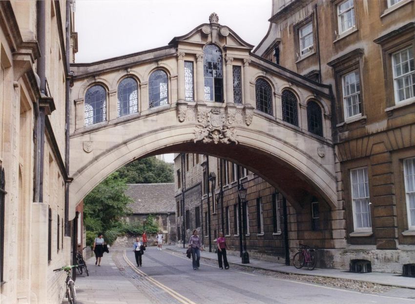
Published as a conference paper at ICLR 2022

loss on the Super-feature attention maps that encourages them to be diverse. An overview of the
pipeline is depicted in Figure 2. We refer to our approach as Feature Integration-based Retrieval or
FIRe for short, an homage to the feature integration theory of Treisman & Gelade (1980).

3.1      L OCAL FEATURE I NTEGRATION T RANSFORMER (LIT)

Inspired by the recent success of attention mechanisms for encoding semantics from global context
in sequences (Vaswani et al., 2017) or images (Caron et al., 2021), we rely on attention to design our
Local feature Integration Transformer (LIT), a module that outputs an ordered set of Super-features.
Let LIT be represented by function ΦpUq : RLˆD Ñ RN ˆd that takes as input the set of local
features U and outputs N Super-features. We define LIT as an iterative module:
                                ΦpUq “ Q T ,       Q t “ φpU; Q t´1 q,                             (3)
                                                                           0    N ˆd
where φ denotes the core function of the module applied T times, and Q P R            denotes a set of
learnable templates, i.e. a matrix of learnable parameters. Super-features are progressively formed
by iterative refinement of the templates, conditioned on the local features from the CNN.
The architecture of the core function φ is inspired by the Transformer architecture (Vaswani et al.,
2017) and is composed of a dot-product attention function ψ, followed by a multi-layer perceptron
(MLP). The dot-product attention function ψ receives three inputs, the key, the value and the query1
which are passed through layer normalization and fed to linear projection functions K, V and Q that
project them to dimensions dk , dv and dq , respectively. In practice, we set dk “dv “dq “d“1024.
The key and value inputs are set as the local features ul P U across all iterations. The query input
is the set of templates Q t “ tqnt P Rd , n “ 1 .. N u. It is initialized as the learnable templates
Q 0 for iteration 0, and is set as the previous output of function φ for the following iterations. After
projecting with the corresponding linear projection functions, the key and the query are multiplied
to construct a set of N attention maps over the local features, i.e., the columns of matrix α P RLˆN ,
while the L rows αl of that matrix can be seen as the responsibility that each of the N templates has
for each local feature l, and is given by2 :
             » fi
               α1
             — .. ffi                      α̂l               e Ml                Kpul q ¨ Qpqnt q
       α “ – . fl P RLˆN , αl “ řL                 , α̂l “ řN          , Mln “        ?           . (4)
                                          i“1  α̂i          n“1 eMln                     d
               αL

The dot product between keys and templates can be interpreted as a tensor of compatibility scores
between local features and templates. These scores are normalized across templates via a softmax
function, and are further turned into attention maps by l1 normalization across all L spatial locations.
This is a common way of approximating a joint normalization function across rows and columns,
also used by Locatello et al. (2020). The input value is first projected with V , re-weighted with the
attention maps and then residually fed to a MLP3 to produce the output of function φ:
   Q t “ φpU; Q t´1 q,              φpU; Qq “ MLPpψpU; Qqq ` ψpU; Qq,                                ψpU; Qq “ V pUq ¨ α ` Q. (5)
Following standard image retrieval practice, we further whiten and l2 -normalize the output of ΦpUq
to get the final set of Super-features. Specifically, let ΦpUq “ rŝ1 ; . . . ; ŝN s P RN ˆd be the raw
output of our iterative attention module, we define the ordered set of Super-features as:
                                  !               opŝn q                )
                             S “ sn : sn “                 , n “ 1, .., N ,                           (6)
                                                }opŝn q}2
where, as in Section 2, op¨q denotes dimensionality reduction and whitening. Figure 2 (right) illus-
trates the architecture of LIT. Note that all learnable parameters of φ are shared across all iterations.
What do Super-features attend to? Each Super-feature in S is a function of all local features
in U, invariant to permutation of its elements, and can thus attend arbitrary regions of the image.
    1
       The term ‘query’ has a precise meaning for retrieval; yet, for this subsection only, we overload the term to refer to one of the inputs of
the dot-product attention, consistently with the terminology from seminal works on attention by Vaswani et al. (2017).
     2
       The attention maps presented in Eq.(4) are technically taken at iteration t, but we omit iteration superscripts for clarity. For the rest of the
paper and visualizations, we use attention maps to refer to the attention maps of Eq.(4) after the final (T -th) iteration of the iterative module.
     3
       The MLP function consists of a layer-norm, a fully-connected layer with half the dimensions of the features, a ReLU activation and a
fully-connected layer that projects features back to their initial dimension.

                                                                          4
Published as a conference paper at ICLR 2022

To visualize the patterns captured by Super-features, Figure 1 shows the attention maps of the same
five Super-features for three images, including two of the same landmark (first two rows). The type
of patterns depends on the learned initialization templates Q 0 ; this explains why the Super-features
form an ordered set, a property which allows to directly compare Super-features with the same ID.
We observe the attention maps to be similar across images of the same landmark and to contain
some mid-level patterns (such as a half-circle on the second column, or windows on the third one).

3.2   L EARNING WITH S UPER - FEATURES

We jointly fine-tune the parameters of the CNN and of the LIT module using contrastive learning.
However, departing from recent approaches like HOW (Tolias et al., 2020) or DELG (Cao et al.,
2020) that use a global contrastive loss similar to the one presented in Eq. (2), we introduce a
contrastive loss that operates directly on Super-features, the representations we use at test time,
and yet only requires image-level labels. Given a positive pair (i.e. matching images of the same
landmark) and a set of negative images, we select promising Super-feature pairs by exploiting their
ordered nature and without requiring any extra supervision signal. We then minimize their pairwise
distance, while simultaneously reducing the spatial redundancy of Super-features within an image.
Selecting matching Super-features. Since we are only provided with pairs of matching images,
i.e. image-level labels, defining correspondences at the Super-feature level is not trivial. Instead
of approximating sophisticated metrics (Liu et al., 2020; Mialon et al., 2021)–see Section 5 for a
discussion–, we leverage the fact that Super-features are ordered and we select promising matches
and filter out erroneous ones only relying on simple, nearest neighbor-based constraints.
For any s P S, let ipsq be the function that returns the position/order or Super-feature ID, i.e.
ipsi q “ i, @si P S. Further let function nps, Sq “ arg minsi PS }s ´ si }2 be the function that
returns the nearest neighbor of s from set S. Now, given a positive pair of images x, x` , let
s P S, s1 P S 1 be two Super-features from their Super-feature sets S, S 1 , respectively. In order for
Super-feature pair ps, s1 q to be eligible, all of the following criteria must be met: a) s, s1 have to be
reciprocal nearest neighbors, b) they need to pass Lowe’s first-to-second neighbor ratio test (Lowe,
2004) and c) they need to have the same Super-feature ID. Let P be the set of eligible pairs and τ
the hyper-parameter that controls the ratio test; the conditions above can formally be written as:
                     "                                  "
       1               s “ nps1 , Sq                     ipsq “ ips1 q
  ps, s q P P ðñ                             and                                                    . (7)
                       s1 “ nps, S 1 q                   }s ´ s1 }2 { }s1 ´ nps1 , Sztsuq}2 ě τ
We set τ “ 0.9. Our ablations (Section 4.1) show that all criteria are important. Note that the pair
selection step is non-differentiable and no gradients are computed for Super-features not in P. We
further discuss this in Appendix B.4 and empirically show that all Super-features are trained.
A contrastive loss on Super-features. Once the set P of all eligible Super-feature pairs has been
constructed, we define a contrastive margin loss on these matches. Let pair p “ ps, s` q P P be a pair
of Super-features, selected from a pair of matching images x, x` , and let Npjq “ tnkj : k “ 1 .. nu
for j “ 1 .. N be the set of Super-features with Super-feature ID j extracted from negative images
py1´ , . . . , yn´ q. The contrastive Super-feature loss can be written as:
                                      ÿ ”›                                           ı
                                             ›s ´ s` ›2 `
                                                      ›       ÿ                  2 `
                                                                      1
                        Lsuper “                       2
                                                                    rµ  ´ }s ´ n}2 s  ,            (8)
                              ps,s` qPP                 nPNpipsqq

where µ1 is a margin hyper-parameter and the negatives for each s are the Super-features from all n
negative images of the training tuple with Super-feature ID equal to ipsq.
Reducing the spatial correlation between attention maps. To obtain Super-features that are as
complementary as possible, we encourage them to attend to different local features, i.e. different
locations of the image. To this end, we minimize the cosine similarity between the attention maps
of all Super-features of every image.
Specifically, let matrix α “ rα̃1 , . . . , α̃N s now be seen as column vectors denoting the N attention
maps after the last iteration of LIT. The attention decorrelation loss is given by:
                                     1        ÿ       α̃|i ¨ α̃j
                   Lattn pxq “                                      ,   i, j P t1, .., N u.           (9)
                                 N pN ´ 1q          }α̃i }2 }α̃j }2
                                              i‰j

                                                    5
Published as a conference paper at ICLR 2022

 reci-     ratio   same   SfM-120k    ROxford       RParis                                                          0.7
 proc.      test    ID       val     med hard      med hard

                                                                                                                          Match ratio
                                                                                                                    0.6
                            68.3     64.3   39.8   74.1   52.4                        With same-ID constraint
 X                          79.6     69.2   44.3   79.2   60.9                        Without same-ID constraint    0.5
 X          X               80.8     70.7   45.1   80.3   61.9                                                      0.4
                    X       75.9     63.8   35.1   77.3   56.5
 X          X       X       89.7     81.8   61.2   85.3   70.0                                                      0.3
                                                                      0          50         100       150         200 Epochs
Table 1: Ablation on matching constraints: Impact                    Figure 3: Evolution of the matching quality mea-
of removing constraints on reciprocity, Lowe’s ratio                 sured as the ratio of matches coming from the positive
test and the Super-feature ID.                                       pair over all pairs with the query in each training tuple.

In other words, this loss minimizes the off-diagonal elements of the N ˆN self-correlation matrix of
α̃. We ablate the benefit of this loss and others components presented in this section in Section 4.1.
Image retrieval with Super-features. Our full pipeline, FIRe, is composed of a model that outputs
Super-features, trained with the contrastive Super-feature loss of Eq.(8) and the attention decorre-
lation loss of Eq.(9). As our ablations show (see Section 4), the combination of these two losses
is required for achieving state-of-the-art performance, while adding a third loss on the aggregated
global features as in Eq.(2) does not bring any gain.

4        E XPERIMENTS

This section validates our proposed FIRe approach on standard landmark retrieval tasks. We use
the SfM-120k dataset (Radenović et al., 2018b) following the 551/162 3D model train/val split
from Tolias et al. (2020). For testing, we evaluate instance-level search on the ROxford (Philbin
et al., 2007) and the RParis (Philbin et al., 2008) datasets in their revisited version (Radenović et al.,
2018a), with and without the 1 million distractor set called R1M. They both contain 70 queries,
with 4993 and 6322 images respectively. We report mean average precision (mAP) on the Medium
(med) and Hard (hard) setups, or the average over these two setups (avg).

Image search with Super-features. At test time, we follow the exact procedure described by
Tolias et al. (2020) and extract Super-features from each image at 7 resolutions/scales {2.0, 1.414,
1.0, 0.707, 0.5, 0.353, 0.25}. We then keep the top Super-features (the top 1000 unless otherwise
stated) according to their L2 norm and use the binary version of ASMK with a codebook of 65536
clusters. Note that one can measure the memory footprint of a database image x via the number of
non-empty ASMK clusters, i.e. clusters with at least one assignment, denoted as |Cpxq|.
Implementation details. We build our codebase on HOW (Tolias et al., 2020)4 and sample tuples
composed of one query image, one positive image and 5 hard negatives. Each epoch is composed
of 400 batches of 5 tuples each, while hard negatives are updated at each epoch using the global
features of Eq.(1). We train our model for 200 epochs on SfM-120k using an initial learning rate of
3.10´5 and random flipping as data augmentation. We multiply the learning rate by a factor of 0.99
at each epoch, and use an Adam optimizer with a weight decay of 10´4 . We use a ResNet50 (He
et al., 2016) without the last convolutional block as backbone (R50´ ). For LIT, we use D “ dk “
dq “ dv “ d “ 1024. Following HOW, we reduce the dimensionality of features to 128 and
initialize op¨q using PCA and whitening before training and keep it frozen. We pretrain the LIT
module with the backbone on ImageNet-1K for image classification, see details in Appendix B.6.
We use µ1 “ 1.1 in Eq.(8) and weight Lsuper and Lattn with 0.02 and 0.1, respectively.

4.1       A NALYSIS AND ABLATIONS

In this section, we analyze the proposed FIRe framework and perform exhaustive ablations on the
training losses and the matching constraints. The impact of the number of iterations (T ) and tem-
plates (N ) in LIT is studied in Appendix A.1. For the rest of the paper, we set T “ 6 and N “ 256.
Matching constraints ablation. Table 1 reports the impact of the different matching constraints:
nearest neighbor, reciprocity, Lowe ratio test and constraint on Super-features ID. Adding reciprocity
     4
         https://github.com/gtolias/how

                                                                 6
Published as a conference paper at ICLR 2022

                                                                                  1          256         1            256
                                                                              1                     1                        low
                                 SfM-120k    ROxford       RParis
 Lglobal       Lattn   Lsuper
                                    val     med hard      med hard

                                                                                                                             Correlation
 X                                 79.0     64.3   38.0   75.4   51.7
 X             X                   87.7     75.8   51.2   79.0   57.0
 X             X       X           88.4     79.0   57.2   83.0   65.6
                       X           61.7     59.3   32.8   69.9   47.3
               X       X           89.7     81.9   61.5   85.3   70.1                                                        high
                                                                            256                    256
Table 2: Ablation on loss components: Im-                                   Figure 4: Impact of Lattn on the correlation
pact of removing Lattn , using either a global loss                         matrix between attention maps (the darker, the
Lglobal or a loss directly on Super-features Lsuper                         lower is the correlation) at the last iteration of
or a combination of both.                                                   LIT when training with (left) and without (right).
                                                                            This is averaged over the 70 queries of ROxford.

                            ROxford (avg)                                                        RParis (avg)
               1000
                                                                                          1000
  70                             2000                                         75
                                                                                                   2000
  65                    1000                                                  70
                                                                                           1000

  60
                                                     FIRe                     65                                     FIRe
                                                     HOW                                                             HOW
           0               500       1,000         1,500                              0     500              1,000   1,500
                  average |Cpxq|                                       average |Cpxq|
Figure 5: Performance versus memory for HOW and FIRe. The x-axis shows the average number
of clusters per image used in ASMK (proportional to memory usage). We vary the number of
features extracted per image before aggregation in t200, . . . , 2000, 2500, . . . , 5000u; solid markers
denote the commonly used settings (1000/2000). FIRe has at most 1,792 features (256 per scale).
and Lowe’s ratio test significantly improves performance, which indicates that it reduces the number
of incorrect matches. Keeping all pairs with the same ID yields lower performance: the ID constraint
alone is not enough. One possible explanation is that two images from the same landmark may differ
significantly, e.g. when some parts are visible in only one of the two images. In that case, the other
constraints allow features attending non-overlapping regions of a positive image pair to be excluded
from P. Finally, combining the selective ID constraint with the others yields the best performance.
In order to better understand the impact of the Super-feature ID constraint, a constraint only applica-
ble for Super-features due to their ordered nature, we measure the quality of selected matches during
training with and without it. Since there is no ground-truth for such localized matches on landmark
retrieval datasets, we measure instead the ratio of matches coming from the positive pair, over all
matches (from the positive and all negatives). Ideally, a minimal number of matches should come
from the negatives, hence this ratio should be close to 1. In Figure 3 we plot this match ratio for all
epochs; we observe that it is significantly higher when using the Super-features ID constraint.
Training losses ablation. We study the impact of the different training losses in Table 2. We start
from a global loss similar to HOW (first row). We then add the decorrelation loss (second row)
and observe a clear gain. It can be explained by the fact that without this loss, Super-features tend
to be redundant (see the correlation matrices in Figure 4). Adding the loss operating directly on
the Super-features further improves performance (third row). Next, we remove the global loss and
keep only the loss on Super-features alone (fourth row) or with the decorrelation loss (last row).
The latter performs best (fourth vs last row). Figure 4 displays the correlation matrix of Super-
features attention maps with and without Lattn . Without it, we observe that most Super-features have
correlated attentions. In contrast, training with Lattn leads to uncorrelated attention maps. This is
illustrated in Figure 1 which shows several attention maps focusing on different areas.
Varying the number of features at test time. Figure 5 compares HOW (Tolias et al., 2020) with
our approach, as we vary the number of local features / Super-features. The x-axis shows the average
number of clusters used in ASMK for the database images, i.e., which is proportional to the average
memory footprint of an image. We observe that our approach does not only significantly improve

                                                                        7
Published as a conference paper at ICLR 2022

                         Scale of selected features (%)                        Features selected per scale(%)                      Total nb. features per scale
                                                                         0.6
                              HOW
    features (%)

                                                          features (%)
                   0.3                                                                                                       4K

                                                                                                                # features
                              FIRe
                                                                         0.4                                                 3K
                   0.2
                                                                                                                             2K
                   0.1                                                   0.2
                                                                                                                             1K
                     0
                         0.25 0.35 0.5 0.7 1.0 1.4 2.0                         0.25 0.35 0.5 0.7 1.0 1.4 2.0                      0.25 0.35 0.5 0.7 1.0 1.4 2.0

Figure 6: Statistics on the feature selected across scales for HOW and FIRe, averaged over the 70
queries from ROxford. Left: Among the 1000 selected features, we show the percentage coming
from each scale. Middle: For each scale, we show the ratio of features that are selected. Right: Total
number of features per scale; we extract N “ 256 Super-features regardless of scale.

accuracy compared to HOW, but also requires overall less memory. Notably, FIRe matches the
best performance of HOW with a memory footprint reduced by a factor of 4. For both methods,
performance goes down once feature selection no longer discards background features. The gain in
terms of performance is even larger when considering a single scale at test time (see Appendix B.1).
Statistics on the number of selected features per scale. The left plot of Figure 6 shows the
percentage of the 1000 selected features that comes from each scale, for HOW and FIRe. For HOW
most selected features come from the higher resolution inputs; by contrast, selected Super-features
are almost uniformly distributed across scales. Interestingly, Figure 6 (middle) shows that HOW
keeps a higher percentage of the features coming from coarser scales. Yet, the final feature selection
for HOW is still dominated by features from higher scales, due to the fact that the number of local
features significantly increases with the input resolution (see Figure 6 right).

4.2                C OMPARISON TO THE STATE OF THE ART

We compare our method to the state of the art in Table 3. All reported methods are trained on
SfM-120k for a fair comparison.5 First, we observe that methods based on global descriptors (Tolias
et al., 2016; Revaud et al., 2019a) compared with a L2 distance tend to be less robust than methods
based on local features (Noh et al., 2017; Tolias et al., 2020). DELG (Cao et al., 2020) shows better
performance, owing to a re-ranking step based on local features, at the cost of re-extracting local
features for the top-ranked images of a given query, given that local features would take too much
memory to store. Our FIRe method outperforms DELF (Noh et al., 2017) as well as HOW (Tolias
et al., 2020) by a significant margin when extracting 1000 features per image. Importantly, our
approach also requires less memory, as it uses fewer ASMK clusters per image, as shown in Figure 5:
for the whole R1M set, HOW uses 469 clusters per image while FIRe uses only 383, on average.

5                  R ELATED W ORK
Image descriptors for retrieval. The first approaches for image retrieval were based on handcrafted
local descriptors and bag-of-words representations borrowed from text retrieval (Sivic & Zisserman,
2003; Csurka et al., 2004), or other aggregation techniques like Fisher Vectors (Perronnin et al.,
2010), VLAD (Jégou et al., 2010) or ASMK (Tolias et al., 2013). First deep learning techniques were
extracting a global vector per image either directly or by aggregating local activations (Gordo et al.,
2016; Radenović et al., 2018b) and have shown to highly outperform handcrafted local features,
see (Csurka & Humenberger, 2018) for a review. Methods that perform matching or re-ranking using
CNN-based local features are currently the state of the art in the area (Noh et al., 2017; Teichmann
et al., 2019; Cao et al., 2020; Tolias et al., 2020). They are able to learn with global (i.e. image-level)
annotations. Most of them use simple variants of attention mechanisms (Noh et al., 2017; Ng et al.,
2020) or simply the feature norm (Tolias et al., 2020) to weight local activations.
Low-level features aggregation. Aggregating local features into regional features has a long his-
tory. Crucial to the success of traditional approaches, popular methods include selecting discrimi-
native patches in the input image (Singh et al., 2012; Gordo, 2015), regressing saliency map scores
        5
      The GLDv2-clean dataset (Yokoo et al., 2020) is sometimes used for training. Yet, there is significant overlap between its training classes
and the ROxford and RParis query landmarks. This departs from standard image retrieval evaluation protocols. See Appendix B.8 for details.

                                                                                        8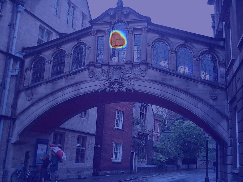
Published as a conference paper at ICLR 2022

                                                   Mem       ROxford          ROxford +R1M           RParis            RParis +R1M
    method                                  FCN
                                                   (GB)    med   hard          med     hard        med    hard         med     hard
    Global descriptors
     RMAC (Tolias et al., 2016)             R101    7.6    60.9      32.4      39.3      12.5      78.9      59.4      54.8      28.0
     AP-GeM; (Revaud et al., 2019a)         R101    7.6    67.1      42.3      47.8      22.5      80.3      60.9      51.9      24.6
     GeM+SOLAR (Ng et al., 2020)            R101    7.6    69.9      47.9      53.5      29.9      81.6      64.5      59.2      33.4
    Global descriptors + reranking with local features
     DELG (Cao et al., 2020)           R50         7.6     75.1      54.2      61.1      36.8      82.3      64.9      60.5      34.8
     DELG (Cao et al., 2020)           R101        7.6     78.5      59.3      62.7      39.3      82.9      65.5      62.6      37.0
    Local features + ASMK matching (max. 1000 features per image)
     DELF (Noh et al., 2017)              R50´  9.2   67.8     43.1            53.8      31.2      76.9      55.4      57.3      26.4
     DELF-R-ASMK (Teichmann et al., 2019) R50´ 27.4   76.0     52.4            64.0      38.1      80.2      58.6      59.7      29.4
     HOW (Tolias et al., 2020)            R50´  7.9   78.3     55.8            63.6      36.8      80.1      60.1      58.4      30.7
     FIRe (ours)                          R50´  6.4   81.8     61.2            66.5      40.1      85.3      70.0      67.6      42.9
         (standard deviation over 5 runs)                 (˘0.6)    (˘1.0)    (˘0.8)    (˘1.1)    (˘0.4)    (˘0.6)    (˘0.7)    (˘0.8)
         (mAP gains over HOW)                             (Ò 3.5)   (Ò 5.4)   (Ò 2.9)   (Ò 3.3)   (Ò 5.2)   (Ò 9.9)   (Ò 9.2)   (Ò 12.2)
Table 3: Comparison to the state of the art. All models are trained on SfM-120k. FCN denotes
the fully-convolutional network backbone, with R50´ denoting a ResNet-50 without the last block.
Memory is reported for the image representation of the full R1M set (without counting local features
for the global descriptors + reranking methods). ; result from (Tolias et al., 2020). Bold denotes
best performance, underlined second best among methods using ASMK, italics second best overall.

at different resolutions (Jiang et al., 2013), aggregating SIFT descriptors with coding and pooling
schemes (Boureau et al., 2010), or mining frequent patterns in sets of SIFT features (Singh et al.,
2012). More recently, Hausler et al. (2021) introduced a multi-scale fusion of patch features.
Supervision for local features. Several works provide supervision at the level of local features in
the context of contrastive learning. Xie et al. (2021) and Chen et al. (2021) obtain several views
of an input image using data augmentations with known pixel displacements. Similarly, Liu et al.
(2020) train a model to predict the probability for a pair of local features to match, evaluated using
known displacements. Wang et al. (2020) and Zhou et al. (2021) obtain local supervision by relying
on epipolar coordinates and relative camera poses. Positive pairs in image retrieval depart from these
setups, as pixel-level correspondences cannot be known. To build matches, Wang et al. (2021) use a
standard nearest neighbor algorithm to build pairs of features, similarly to our approach, but without
the use of filtering which is critical to our final performance. Using the current model predictions
to define targets is reminiscent of modern self-supervised learning approaches which learn without
any label (Caron et al., 2021; Grill et al., 2020). The additional filtering step can be seen as a way to
keep only the most reliable model predictions, similar to self-distillation as in e.g. Sohn et al. (2020).
Attention modules. Our LIT module is an iterative variant of standard attention (Bahdanau et al.,
2015; Vaswani et al., 2017), adapted to map a variable number of input features to an ordered set
of N output features, similar to Lee et al. (2019). The Perceiver model (Jaegle et al., 2021) has
demonstrated the flexibility of such constructions by using it to scale attention-based deep networks
to large inputs. Our design was heavily inspired by slot-attention (Locatello et al., 2020), but has
some key differences that enable us to achieve high performance in more complex visual environ-
ments: a) unlike the slot attention which initializes its slots with i.i.d sampling, we learn the initial
templates and therefore define an ordering on the output set, a crucial property for selecting promis-
ing matches; b) we replace the recurrent network gates with a residual connection across iterations.
These modifications, together with the attention decorrelation loss enable our module to go from a
handful of object-oriented slots to a much larger set of output features. For object detection, Carion
et al. (2020) rely on a set of learned object queries to initialize a stack of transformer layers. Unlike
ours, their module is not recurrent; Appendix A.1 experimentally shows substantial benefits from
applying LIT T times, with weight sharing, to increase model flexibility without extra parameters.

6       C ONCLUSIONS
We present an approach that aggregates local features into Super-features for image retrieval, a task
that has up to now been dominated by approaches that work at the local feature level. We design an
attention mechanism that outputs an ordered set of such features that are more discriminative and
expressive than local features. Exploiting their ordered nature and without any extra supervision, we
present a loss working directly on the proposed features. Our method not only significantly improves
performance, but also requires less memory, a crucial requirement for scalable image retrieval.

                                                                    9
Published as a conference paper at ICLR 2022

R EFERENCES
Artem Babenko and Victor Lempitsky. Aggregating deep convolutional features for image retrieval. In Proc.
  ICCV, 2015.

Dzmitry Bahdanau, Kyunghyun Cho, and Yoshua Bengio. Neural machine translation by jointly learning to
  align and translate. In Proc. ICLR, 2015.

Y-Lan Boureau, Francis Bach, Yann LeCun, and Jean Ponce. Learning mid-level features for recognition. In
  Proc. CVPR, 2010.

Bingyi Cao, André Araujo, and Jack Sim. Unifying deep local and global features for image search. In Proc.
  ECCV, 2020.

Nicolas Carion, Francisco Massa, Gabriel Synnaeve, Nicolas Usunier, Alexander Kirillov, and Sergey
  Zagoruyko. End-to-end object detection with transformers. Proc. ECCV, 2020.

Mathilde Caron, Hugo Touvron, Ishan Misra, Hervé Jégou, Julien Mairal, Piotr Bojanowski, and Armand
  Joulin. Emerging properties in self-supervised vision transformers. In Proc. ICCV, 2021.

Kai Chen, Lanqing Hong, Hang Xu, Zhenguo Li, and Dit-Yan Yeung. Multisiam: Self-supervised multi-
  instance siamese representation learning for autonomous driving. In Proc. ICCV, 2021.

Yunpeng Chen, Marcus Rohrbach, Zhicheng Yan, Yan Shuicheng, Jiashi Feng, and Yannis Kalantidis. Graph-
  based global reasoning networks. In Proc. CVPR, 2019.

Gabriela Csurka and Martin Humenberger. From handcrafted to deep local invariant features. arXiv preprint
  arXiv:1807.10254, 2018.

Gabriela Csurka, Christopher Dance, Lixin Fan, Jutta Willamowski, and Cédric Bray. Visual categorization
  with bags of keypoints. In Proc. ECCV Worshops, 2004.

Albert Gordo. Supervised mid-level features for word image representation. In Proc. CVPR, 2015.

Albert Gordo, Jon Almazán, Jerome Revaud, and Diane Larlus. Deep image retrieval: Learning global repre-
  sentations for image search. In Proc. ECCV, 2016.

Jean-Bastien Grill, Florian Strub, Florent Altché, Corentin Tallec, Kavukcuoglu Koray, Rémi Munos, and
   Michal Valko. Bootstrap your own latent: A new approach to self-supervised learning. In Proc. NeurIPS,
   2020.

Stephen Hausler, Sourav Garg, Ming Xu, Michael Milford, and Tobias Fischer. Patch-netvlad: Multi-scale
   fusion of locally-global descriptors for place recognition. In Proc. CVPR, 2021.

Kaiming He, Xiangyu Zhang, Shaoqing Ren, and Jian Sun. Deep residual learning for image recognition. In
  Proc. CVPR, 2016.

Martin Humenberger, Yohann Cabon, Nicolas Guerin, Julien Morat, Jérôme Revaud, Philippe Rerole, Noé
  Pion, Cesar de Souza, Vincent Leroy, and Gabriela Csurka. Robust image retrieval-based visual localization
  using kapture. arXiv preprint arXiv:2007.13867, 2020.

Andrew Jaegle, Felix Gimeno, Andrew Brock, Andrew Zisserman, Oriol Vinyals, and Joao Carreira. Perceiver:
  General perception with iterative attention. In Proc. ICML, 2021.

Hervé Jégou, Matthijs Douze, Cordelia Schmid, and Patrick Pérez. Aggregating local descriptors into a compact
  image representation. In Proc. CVPR, 2010.

Huaizu Jiang, Jingdong Wang, Zejian Yuan, Yang Wu, Nanning Zheng, and Shipeng Li. Salient object detec-
  tion: A discriminative regional feature integration approach. In Proc. CVPR, 2013.

Juho Lee, Yoonho Lee, Jungtaek Kim, Adam R. Kosiorek, Seungjin Choi, and Yee Whye Teh. Set transformer
  a framework for attention-based permutation-invariant neural networks. In Proc. ICML, 2019.

Songtao Liu, Zeming Li, and Jian Sun. Self-emd: Self-supervised object detection without imagenet. arXiv
  preprint arXiv:2011.13677, 2020.

Francesco Locatello, Dirk Weissenborn, Thomas Unterthiner, Aravindh Mahendran, Georg Heigold, Jakob
   Uszkoreit, Alexey Dosovitskiy, and Thomas Kipf. Object-centric learning with slot attention. In Proc.
   NeurIPS, 2020.

                                                      10
Published as a conference paper at ICLR 2022
David G Lowe. Distinctive image features from scale-invariant keypoints. IJCV, 2004.
Grégoire Mialon, Dexiong Chen, Alexandre d’Aspremont, and Julien Mairal. A trainable optimal transport
embedding for feature aggregation and its relationship to attention. In Proc. ICLR, 2021.
Tony Ng, Vassileios Balntas, Yurun Tian, and Krystian Mikolajczyk. Solar: second-order loss and attention for
image retrieval. In Proc. ECCV, 2020.
Hyeonwoo Noh, Andre Araujo, Jack Sim, Tobias Weyand, and Bohyung Han. Large-scale image retrieval with
attentive deep local features. In Proc. ICCV, 2017.
Florent Perronnin, Yan Liu, Jorge Sánchez, and Hervé Poirier. Large-scale image retrieval with compressed
fisher vectors. In Proc. CVPR, 2010.
James Philbin, Ondrej Chum, Michael Isard, Josef Sivic, and Andrew Zisserman. Object retrieval with large
vocabularies and fast spatial matching. In Proc. CVPR, 2007.
James Philbin, Ondrej Chum, Michael Isard, Josef Sivic, and Andrew Zisserman. Lost in quantization: Im-
proving particular object retrieval in large scale image databases. In Proc. CVPR, 2008.
Filip Radenović, Ahmet Iscen, Giorgos Tolias, Yannis Avrithis, and Ondřej Chum. Revisiting oxford and paris:
Large-scale image retrieval benchmarking. In Proc. CVPR, 2018a.
Filip Radenović, Giorgos Tolias, and Ondřej Chum. Fine-tuning cnn image retrieval with no human annotation.
IEEE Trans PAMI, 2018b.
Jerome Revaud, Jon Almazán, Rafael S Rezende, and Cesar Roberto de Souza. Learning with average precision:
Training image retrieval with a listwise loss. In Proc. ICCV, 2019a.
Jerome Revaud, Cesar De Souza, Martin Humenberger, and Philippe Weinzaepfel. R2D2: Reliable and repeat-
able detector and descriptor. In Proc. NeurIPS, 2019b.
Torsten Sattler, Will Maddern, Carl Toft, Akihiko Torii, Lars Hammarstrand, Erik Stenborg, Daniel Safari,
Masatoshi Okutomi, Marc Pollefeys, Josef Sivic, et al. Benchmarking 6dof outdoor visual localization in
changing conditions. In Proc. CVPR, 2018.
Saurabh Singh, Abhinav Gupta, and Alexei A Efros. Unsupervised discovery of mid-level discriminative
patches. In Proc. ECCV, 2012.
Josef Sivic and Andrew Zisserman. Video google: A text retrieval approach to object matching in videos. In
Proc. ICCV, 2003.
Kihyuk Sohn, David Berthelot, Chun-Liang Li, Zizhao Zhang, Nicholas Carlini, Ekin D. Cubuk, Alex Ku-
rakin, Han Zhang, and Colin Raffel. Fixmatch: Simplifying semi-supervised learning with consistency and
confidence. Proc. NeurIPS, 2020.
Marvin Teichmann, Andre Araujo, Menglong Zhu, and Jack Sim. Detect-to-retrieve: Efficient regional aggre-
gation for image search. In Proc. CVPR, 2019.
Giorgos Tolias, Yannis Avrithis, and Hervé Jégou. To aggregate or not to aggregate: Selective match kernels
for image search. In Proc. ICCV, 2013.
Giorgos Tolias, Ronan Sicre, and Hervé Jégou. Particular object retrieval with integral max-pooling of cnn
activations. In Proc. ICLR, 2016.
Giorgos Tolias, Tomas Jenicek, and Ondřej Chum. Learning and aggregating deep local descriptors for instance-
level recognition. In Proc. ECCV, 2020.
Anne M Treisman and Garry Gelade. A feature-integration theory of attention. Cognitive psychology, 1980.
Ashish Vaswani, Noam Shazeer, Niki Parmar, Jakob Uszkoreit, Llion Jones, Aidan N Gomez, Łukasz Kaiser,
and Illia Polosukhin. Attention is all you need. In Proc. NeurIPS, 2017.
Qianqian Wang, Xiaowei Zhou, Bharath Hariharan, and Noah Snavely. Learning feature descriptors using
camera pose supervision. In Proc. ECCV, 2020.
Xinlong Wang, Rufeng Zhang, Chunhua Shen, Tao Kong, and Lei Li. Dense contrastive learning for self-
supervised visual pre-training. In Proc. CVPR, 2021.
11Published as a conference paper at ICLR 2022
Tobias Weyand, Andre Araujo, Bingyi Cao, and Jack Sim. Google landmarks dataset v2-a large-scale bench-
mark for instance-level recognition and retrieval. In Proc. CVPR, 2020.
Tianjun Xiao, Yichong Xu, Kuiyuan Yang, Jiaxing Zhang, Yuxin Peng, and Zheng Zhang. The application of
two-level attention models in deep convolutional neural network for fine-grained image classification. In
Proc. CVPR, 2015.
Zhenda Xie, Yutong Lin, Zheng Zhang, Yue Cao, Stephen Lin, and Han Hu. Propagate yourself: Exploring
pixel-level consistency for unsupervised visual representation learning. In Proc. CVPR, 2021.
Shuhei Yokoo, Kohei Ozaki, Edgar Simo-Serra, and Satoshi Iizuka. Two-stage discriminative re-ranking for
large-scale landmark retrieval. In Proc. CVPR Worshops, 2020.
Qunjie Zhou, Torsten Sattler, and Laura Leal-Taixe. Patch2pix: Epipolar-guided pixel-level correspondences.
In Proc. CVPR, 2021.
12Published as a conference paper at ICLR 2022
Appendix
Table of Contents
A Additional ablations 14
A.1 Impact of the iteration and the number of templates hyper-parameters . . . . . . 14
A.2 Impact of hard negatives . . . . . . . . . . . . . . . . . . . . . . . . . . . . . . 14
A.3 Impact of the update function . . . . . . . . . . . . . . . . . . . . . . . . . . . 15
A.4 Extended ablation on matching constraints . . . . . . . . . . . . . . . . . . . . 15
A.5 Impact of the template initialization . . . . . . . . . . . . . . . . . . . . . . . . 15
B Analysis and discussions 16
B.1 Single-scale results . . . . . . . . . . . . . . . . . . . . . . . . . . . . . . . . 16
B.2 Consistency of attention maps across scales . . . . . . . . . . . . . . . . . . . . 16
B.3 Redundancy in Super-features . . . . . . . . . . . . . . . . . . . . . . . . . . . 16
B.4 Are all Super-features trained? . . . . . . . . . . . . . . . . . . . . . . . . . . 17
B.5 Using the Super-feature loss with local features . . . . . . . . . . . . . . . . . . 17
B.6 Pretraining the backbone together with LIT . . . . . . . . . . . . . . . . . . . . 18
B.7 Computational cost of Super-features extraction . . . . . . . . . . . . . . . . . 18
B.8 Is Google Landmarks v2 clean an appropriate training dataset for testing on
ROxford and RParis? . . . . . . . . . . . . . . . . . . . . . . . . . . . . . . . 18
C Application to visual localization 18
In this appendix, we present additional ablations (Appendix A), a deeper analysis of our framework
(Appendix B) as well as results of the application of our FIRe framework for image retrieval to
the task of visual localization (Appendix C). We briefly summarize the findings in the following
paragraphs.
Ablations. We study the impact of some hyper-parameters of our model, namely the size N of
the set of Super-features, and the number of iterations T in the LIT module, in Appendix A.1.
We show that 256 Super-features and 6 iterations offer the best trade-off between performance and
computational cost. We also show in Appendix A.2 that we obtain further performance gains of over
1% by increasing the number of negatives to 10 or 15. We then study the impact of replacing the
residual connection inside the LIT module by a recurrent network (Appendix A.3). In Appendix A.4
we present an extended version of Table 1 with further matching constraints and we finally study the
impact of the template initialization on performance in Appendix A.5.
Properties of Super-features. We show single-scale results in Appendix B.1. In Appendix B.2,
we display the attention maps of Super-features, at different scales for a fixed Super-feature ID.
We further study the amount of redundancy in Super-features, compared to local features, in Ap-
pendix B.3. Next, we verify in Appendix B.4 that all Super-features receive training signal, as a
sanity check. We discuss the case of applying a loss directly on local features in Appendix B.5 and
give details about the pretraining on ImageNet in Appendix B.6. In Appendix B.7 we report the
average extraction time for the proposed Super-features, while in Appendix B.8 we discuss the fact
that there is an overlap between the queries from the common ROxford and RParis datasets and the
Google Landmarks-v2-clean dataset that is commonly used as training set for retrieval on ROxford
and RParis.
Application to visual localization. We further evaluate our model using a visual localization setting
on the Aachen Day-Night v1.1 dataset (Sattler et al., 2018) in Appendix C. To do so, we leverage a
retrieval + local feature matching pipeline, and show that it is beneficial to use our method, especially
in hard settings.
13Published as a conference paper at ICLR 2022
A A DDITIONAL ABLATIONS
A.1 I MPACT OF THE ITERATION AND THE NUMBER OF TEMPLATES HYPER - PARAMETERS
In this section, we perform ablations on the number of Super-features N and the number of iterations
T in the Local feature Integration Transformer. We first study the impact of the number N of Super-
features extracted for each scale of each image in Figure 7a. We observe that the best value is 256 on
both the validation and test sets (ROxford and RParis). We then study the impact of the number of
iterations T in Figure 7b. While the performance decreases when doing 2 or 3 iterations compared to
just 1, a better performance is reached for 6 iterations, after which the performance saturates while
requiring more computations. We thus use T “ 6.
SfM-120k val. ROxford (avg) RParis (avg)
90 90
80 80
mAP
mAP
70 70
60
60
64 128 256 512 1024 1 2 3 4 6 9 12
number of templates (N) number of iterations (T)
(a) Impact of the number of Super-features (b) Impact of the number of iterations
Figure 7: Varying the number of Super-features N and of iterations T in the Local feature
Integration Transformer.
A.2 I MPACT OF HARD NEGATIVES
Each training tuple is composed of one image pair depicting the same landmark, and 5 negative
images (i.e. from different landmarks). We plot the performance when varying this number in Fig-
ure 8. We observe that adding more negatives improves overall the performance on all datasets, i.e.
by more than 1% when increasing it to 10 or 15 negatives, but at the cost of a longer training time
as more images need to be processed at each iteration. This is why we use 5 negatives in the rest of
the paper as it offers a good compromise between performance and cost.
SfM-120k val. ROxford (avg) RParis (avg)
90
80
mAP
70
60
1 2 3 4 5 7 10 15
number of negatives per tuple
Figure 8: Varying the number of hard negatives per training tuple.
14Published as a conference paper at ICLR 2022
A.3 I MPACT OF THE UPDATE FUNCTION
The formula for ψ in Equation (5) sums the previous Q with the output of the attention component
V pUq ¨ α, i.e., with a residual connection. This is a different choice than the one made in the
object-centric slot attention of Locatello et al. (2020), which proposes to use a Gated Recurrent
Unit: ψpU; Qq “ GRUpV pUq ¨ α, Q ). We thus compare the residual connection we use to a GRU
function and report results in Table 4 with T “ 3. We observe that the residual connection reaches
a better performance in all datasets while having the interest of not adding extra parameters.
update SfM-120k ROxford RParis
function val med hard med hard
residual 79.9 71.3 43.9 78.7 59.4
GRU 74.7 66.7 41.4 77.2 57.8
Table 4: Impact of the update function in the LIT module. We compare the performance of the
residual combination of the previous template value with the cross-attention tensor compared to a
GRU as used in slot attention (Locatello et al., 2020). In this experiment, we use T “ 3.
In summary, we propose the LIT module to obtain a few hundred features for image retrieval
while slot attention handles a handful of object attentions. Technical differences to the slot attention
include: a) we use a learned initialization of the templates instead of i.i.d. sampling, which allows to
obtain an ordered set of features, and thus to apply the constraint on the ID for the matching, leading
to a clear gain, see Table 1 and Figure 3, b) to handle a larger number of templates, we also add a
decorrelation loss on the attention maps, which has clear benefit, see Table 2 and Figure 4, c) we use
a residual connection with 6 iterations instead of a GRU, leading to improved performance for our
task (see Table 4).
A.4 E XTENDED ABLATION ON MATCHING CONSTRAINTS
reci- ratio same SfM-120k ROxford RParis
proc. test ID val med hard med hard
68.3 64.3 39.8 74.1 52.4
X 79.6 69.2 44.3 79.2 60.9
X X 89.9 81.9 61.1 85.1 69.6
X 73.5 64.6 39.0 75.5 55.0
X X 84.2 75.0 49.8 79.4 61.1
X X 80.8 70.7 45.1 80.3 61.9
X 75.9 63.8 35.1 77.3 56.5
X X X 89.7 81.8 61.2 85.3 70.0
Table 5: Extended ablation on matching constraints. We study the impact of removing constraints
on reciprocity, Lowe’s ratio test and the Super-feature ID.
We show in Table 5 an extended version of Table 1 of the main paper, where we evaluate all possible
combinations of constraints among reciprocity, Lowe’s ratio test and the Super-feature ID. We ob-
serve that the reciprocity constraint and the Super-feature ID constraint are the two most important
ones, while the Lowe’s ratio only only brings a small improvement.
A.5 I MPACT OF THE TEMPLATE INITIALIZATION
In the LIT module, initial templates Q 0 P RN ˆd are learned together with the LIT module. We can
therefore assume that they are adapted to the task at hand. To explore the sensitivity to the initial
templates, we run a variant of FIRe where the initializations are not fine-tuned, but instead frozen
to the values after pretraining on ImageNet. We report performance in Table 6. We observe that
the two variants perform overall similarly. This ablation suggests that the initial templates are up to
some point transferable to other tasks.
15Published as a conference paper at ICLR 2022
Template SfM-120k ROxford RParis
Initialization val med hard med hard
Frozen from ImageNet pretraining 89.5 81.3 59.6 85.3 70.2
Fine-tuned for landmark retrieval 89.7 81.8 61.2 85.3 70.0
Table 6: Fine-tuning the initial templates. Comparison where we either fine-tune the initial tem-
plates Q 0 of LIT (bottom row, as in the main paper) or keep them frozen after ImageNet pretraining
(top row).
ROxford (avg) RParis (avg)
60
55 200 200
50 50
45 200 200
40
40 HOW HOW
35 FIRe FIRe
30
0 50 100 150 200 250 0 50 100 150 200 250
average |Cpxq| average |Cpxq|
Figure 9: Performance versus memory when varying the number of selected features at a
single scale for HOW and FIRe. The x-axis represents the average number of vectors per image
in ASMK, which is proportional to the memory, when varying the number of selected features in
p25, 50, 100, 150, 200, 300, 400, 500, 600q, FIRe is limited to 256 features.
B A NALYSIS AND DISCUSSIONS
B.1 S INGLE - SCALE RESULTS
Similar to Figure 5 of the main paper, we perform the same ablation in Figure 9 when extracting
features at a single scale (1.0). We observe that FIRe significantly improves the mAP on the two
datasets compared to HOW. The average number of clusters, i.e. the memory footprint of images,
remains similar for both methods at a same number of selected features. This stands in contrast to
the multi-scale case where our approach allows to save memory (about 20%), which we hypothesize
is due to the correlation of our features across scales that we discuss below.
B.2 C ONSISTENCY OF ATTENTION MAPS ACROSS SCALES
At test time, we extract Super-features at different image resolutions. We propose here to study if
the attention maps of the Super-features across different image scales are correlated. We show in
Figure 10 the attention maps at the last iteration of LIT for the different image scales. We observe
that they fire at the same image location at the different scales. Note that the attention maps are
larger/smoother at small scales (right columns), as for visualization, we resize lower resolution
attention maps to the original image size.
B.3 R EDUNDANCY IN S UPER - FEATURES
To evaluate the redundancy of Super-features versus local features, Figure 11 displays the aver-
age cosine similarity between every local feature / Super-feature and its K nearest local features /
Super-features from the same image, for different values of K. We observe that Super-features are
significantly less correlated to the most similar other ones, compared to local features used in HOW.
16You can also read