Lineage: Visualizing Multivariate Clinical Data in Genealogy Graphs
←
→
Page content transcription
If your browser does not render page correctly, please read the page content below

1

                       Lineage: Visualizing Multivariate
                      Clinical Data in Genealogy Graphs
                             Carolina Nobre, Nils Gehlenborg, Hilary Coon, and Alexander Lex

      Abstract—The majority of diseases that are a significant challenge for public and individual heath are caused by a combination of
      hereditary and environmental factors. In this paper we introduce Lineage, a novel visual analysis tool designed to support domain experts
      who study such multifactorial diseases in the context of genealogies. Incorporating familial relationships between cases with other data
      can provide insights into shared genomic variants and shared environmental exposures that may be implicated in such diseases. We
      introduce a data and task abstraction, and argue that the problem of analyzing such diseases based on genealogical, clinical, and genetic
      data can be mapped to a multivariate graph visualization problem. The main contribution of our design study is a novel visual
      representation for tree-like, multivariate graphs, which we apply to genealogies and clinical data about the individuals in these families.
      We introduce data-driven aggregation methods to scale to multiple families. By designing the genealogy graph layout to align with a
      tabular view, we are able to incorporate extensive, multivariate attributes in the analysis of the genealogy without cluttering the graph. We
      validate our designs by conducting case studies with our domain collaborators.

      Index Terms—Multivariate networks, biology visualization, genealogies, hereditary genetics, multifactorial diseases.

                                                                                F

1    I NTRODUCTION
      TUDYING ancestry and familial relationships, i.e., genealogies,               have developed in collaboration with psychiatrists and geneticists
S    is both a pasttime enjoyed by amateurs and a research area for
professionals [53]. It is hence not surprising that there are numerous
                                                                                    studying the genetic underpinnings and the environmental factors
                                                                                    of suicide and autism. We use data from the Utah Population
tools to record and visualize genealogies. Yet, most of these tools                 Database1 , a uniquely rich resource for population-based analysis
focus on analyzing family structures for historical purposes, and                   of hereditary diseases.
only a few target a clinical use case of analyzing genealogies                           We contribute a novel technique to visualize large, tree-
in the context of complex, hereditary diseases. Geneticists, on                     like graphs (rooted, directed graphs that have some cycles but
the other hand, have long used genealogical graphs to study how                     are predominantly in tree form) associated with rich numerical,
a genetic disease manifests itself in families. They use drawing                    categorical, and textual attributes. Our approach leverages the tree-
conventions and standardized symbols to show both the family                        like structure of the graphs to produce a linearized layout that
structure and the phenotype, i.e., the observable characteristics                   enables the direct association of the nodes with rich attributes in
of an individual [6]. These charts can provide insights about                       a tightly integrated tabular visualization. We address the issue of
the heritability and segregation patterns of genetic diseases. In                   scalability by introducing novel forms of degree-of-interest-based
their current form, however, they are predominantly useful for                      aggregation that preserve the structure of the graph, and, if desired,
Mendelian diseases, or genetic diseases caused by a small number                    also provide an overview of the attributes of aggregated individu als.
of mutations. Complex diseases such as cancer, autism, diabetes,                    We demonstrate our technique in the context of genealogical data,
obesity, and psychiatric conditions such as depression or suicide,                  and we argue that it can be equally applied to other multivariate
are known to have hereditary components that are regulated by                       trees or tree-like graphs.
a multitude of genes, each having a modest effect on risk, and                           We also contribute a detailed characterization of the domain
also to depend strongly on environmental conditions and chance.                     problems and the domain data as they are encountered when
When studying these conditions in a population, it is imperative to                 analyzing large, clinical genealogies2 and a set of task and
simultaneously consider genetic similarities, shared characteristics                data abstractions derived from these characterizations. Finally,
of the phenotype, and environmental conditions. Also, for these                     we contribute the open-source Lineage visualization tool (https:
polygenic conditions, one needs to consider significantly larger                    //lineage.caleydoapp.org), shown in Figure 1, which implements
populations to reason about hereditary relationships and pursue the                 the technique, and describe multiple design decisions tailored to
discovery of genetic risk mutations.                                                genealogical data visualization.
     Current medical or historical genealogy visualization tools are                     Lineage is in the process of being adopted by our collaborators,
ill equipped to help researchers find patterns in these large, highly               and has undergone iterative design refinements. We have also
multivariate graphs of families and their rich medical histories. In                demonstrated it to other research groups working with genealogical
this paper, we present a novel genealogy visualization tool that we                 and genetic data and have encountered overwhelming enthusiasm.
                                                                                    We validate this work in an illustrative usage scenario and through
•   Carolina Nobre and Alexander Lex are with the University of Utah. E-mail:       qualitative user feedback from domain experts.
    {cnobre, alex}@sci.utah.edu
•   Hilary Coon is with the University of Utah. E-Mail: hilary.coon@utah.edu          1. https://healthcare.utah.edu/huntsmancancerinstitute/research/updb/
•   Nils Gehlenborg is with Harvard Medical School. E-mail: nils@hms.
                                                                                      2. The terms genealogy and pedigree can be used interchangeably in this
    harvard.edu.
                                                                                    context. However, for simplicity, we will always use genealogy.
2

Fig. 1. Lineage visualizing the genealogy of two families with increased numbers of suicides. The genealogy view shows the family relationships in a
linear tree layout, where each node corresponds to a row in the associated table. Suicide cases are highlighted in blue, and a glyph next to the nodes
indicates whether individuals were diagnosed with a personality disorder. The branches use different levels of aggregation (hidden, aggregated,
expanded). The table shows detailed attributes about individuals, or, when branches are aggregated, for groups of individuals.

2    D OMAIN BACKGROUND AND DATA                                            provides genealogical data. Genealogies describe the familial
                                                                            relationships of individuals across multiple generations.
Our collaborators study the genetic underpinnings and the environ-
mental factors influencing psychiatric conditions, such as autism               Figure 2 shows two genealogies using standardized drawing
and suicide, using detailed genealogical, clinical, and genetic             conventions [6]. Females are drawn as circles, males as squares.
data. In this paper, we will focus on suicide, yet our methods              Couples are connected by an edge, and children connect to this
are easily transferable to other complex, multifactorial conditions         edge using orthogonally routed links. The vertical position of
and diseases. Suicide is a high-impact application, as it is one of         nodes is given by their generation. A phenotype of interest is
the leading causes of life-years lost [76] and the 10th most common         marked by a filled-in node. When studying family relationships, a
cause of death in the United States [56]. Suicide is believed to            common approach is to draw family trees considering the ancestry
be caused by a complex combination of risk factors, including               of an individual. Figure 2(a), for example, shows the family of the
environmental stressors and genetic vulnerability. Aggregated data          woman marked in black. The genealogy includes her two siblings
across multiple large studies has produced a heritability estimate          and traces her family tree for two generations to include parents,
of completed suicide of 45% [51], [61]. Genetic risk factors for            uncles and aunts, and grandparents.
suicide are complex and can be classified as multiple subtypes.                 In contrast, our collaborators are interested in understanding
These subtypes often are characterized by co-occurring psychiatric          genetic relationships between individuals afflicted with a condition
conditions (comorbidities) and/or a combined risk of psychiatric            and hence care about individuals who share genetic variants. They
diagnosis. For example, the genetic risk for schizophrenia is also          select families for study that have a statistically increased rate of
associated with a risk for suicide [68].                                    a condition. These family trees are constructed by tracing cases
    Our collaborators have compiled a unique dataset of suicide             back to a “founder”, as illustrated in Figure 2(b). The underlying
cases, including DNA and clinical profiles on 4,017 cases. These            hypothesis is that such founders have genetic risk variants that
cases are linked to the Utah Population Database (UPDB), which              they passed on to their descendants. Within the genealogy, the
3

                                                   Founder                  at the University of Utah. Six domain experts participated in
                                                                            the project. We loosely followed the design study methodology
                                                                            proposed by Sedlmair et al. [64]. Our “discover” phase consisted
                                                                            of multiple meetings with individual collaborators and with the
                                                                            whole group as a team, studying the domain literature and the tools
                                                                            they currently use.
                                                                                We also ran a creativity workshop, specifically the wishful
             (a)                                  (b)
                                                                            thinking component described by Goodwin et al. [24], involving all
                                                                            the collaborators. In the workshop, we asked participants to think
Fig. 2. Two genealogies using standardized symbols focusing on different    about the analysis of suicide data and then discuss in small groups
aspects of the family structure. Females are shown as circles, males as
squares. Individuals with a phenotype of interest are filled-in in black.   and take notes on post-its about what it is they would like to know,
(a) A genealogy showing the family of the female in black, including        see, and do. This idea-generation phase was followed by a phase
siblings, parents, uncles/aunts, and grandparents. (b) A genealogy          in which the teams had to prioritize their insights and then finally
based on a founder, tracing down generations to include the families
of individuals with a phenotype of interest (black).
                                                                            give the whole team an overview of their key ideas. We recorded
                                                                            the workshop and transcribed both the audio and the post-its. We
likelihood of genetic homogeneity is increased, and is more easily          then coded the artifacts and three themes emerged: the data, the
detected through the repeated occurrence of the genetic risk variant        factors involved in suicide, and the analysis tasks. The insights on
in the familial cases. Note that this genealogy contains only               the data and the factors involved in suicide were described in the
individuals who are descendants of one founder and his or her               previous section.
spouse, with the exception of spouses of descendants. Also, the                 The overarching goal of our collaborators is to gain a better
dataset contains only individuals with direct links to a case; i.e.,        understanding of the determining or associated factors of suicide.
siblings, descendants, and direct ancestors are included, whereas,          Our collaborators classify the factors associated with suicide into
for example, uncles/aunts and cousins are not.                              comorbidities and demographic, genetic, and environmental factors.
    The dataset our collaborators have compiled contains about              Specifically, they are interested in identifying and defining detailed
19,000 suicide cases, including 4,585 recent cases with detailed            phenotypes associated with suicide and the degree to which these
data, backed by family structures made up of 118,000 individ-               phenotypes are familial. By finding people who are similar to each
uals from 551 families. Suicide is frequently associated with               other in a relevant way, our collaborators hope to reason about
psychiatric comorbidities, i.e., co-occurring chronic conditions,           genetic homogeneity, i.e., shared genetic factors contributing to
such as depression, bipolar disorder, substance abuse, PTSD,                suicide. They currently rely only on familial structure as a proxy for
or schizophrenia [68]. Also, nonpsychiatric conditions such as              genetic homogeneity. However, they recognize that this approach is
asthma [30] may play a role in some cases. Environmental factors,           limited both as too broad — it is possible that they should consider
such as socioeconomic status, pollution, and seasonality, are also          only a part of a family — and as too narrow — people outside
known to be factors in suicide [2]. To capture this information,            a family who have a similar phenotype could also have a similar
our datasets include demographic variables such as gender, race,            genotype. Robust and detailed phenotypes are, of course, also
age at death, method of death, family demographics (marriage,               interesting by themselves, because they can be used, for example,
divorce, number of siblings/children), and place of residence at the        as part of a risk assessment in a clinical context.
time of death. The datasets also include records of other diagnoses             It is important to note that the contextual knowledge of a
captured as codes from the International Classification of Diseases         researcher is beneficial to the task of classifying a phenotype. For
(ICD) systems, the frequency with which these diagnoses were                example, a diagnosis of depression is weighted differently if it
made, and the time of the first diagnosis.                                  is diagnosed dozens of times and was first diagnosed early in a
    To summarize, each of our many graphs describes a family,               patient’s life. Similarly, a young person who commits suicide in
with individuals as nodes and family relationships as edges. Since          a rural community is unlikely to have a detailed medical history.
the graphs are constructed by tracing ancestry to a founder, they are       Hence, such a case could be similar to others, even if certain
predominantly tree-like, but they do include cycles, for example,           phenotypes are not recorded, if other factors, such as a close
when two cousins have offspring. In addition, we have attributes on         familial relationship, indicate it.
the individuals/nodes in the graphs of various data types, including
                                                                                Our collaborators need a visualization tool that is embedded in
numerical, categorical, temporal, geographic, and textual data.
                                                                            a larger analysis process, one that includes calculating statistically
These attributes are often sparse because only about 10% of
                                                                            significant familial risk (upstream) and searching for shared genetic
individuals in the dataset have committed suicide, and our detailed
                                                                            variants (downstream). They need a tool that focuses on finding
records extend to only about 2% (4,017) of individuals across all
                                                                            individuals and families that are “interesting” with respect to both
families. These detailed records capture about 3,000 dimensions
                                                                            their relatedness and their attributes, which can then be used in
that contain demographic information and information about the
                                                                            further analysis and validation.
manner of death, but predominantly contain comorbidities in the
                                                                                We identified the following domain tasks as the most important
form of disease codes and the time and frequency of these diagnosis.
                                                                            aspects in the workflow of our collaborators:
These dimensions are themselves often sparse because, among
other reasons, a colloquial diagnosis such as “depression” can be           T1 Select families of interest. The analysts want to select a
recorded using one of about 30 ICD codes.                                      family by browsing, by selecting a specific family based on
                                                                               prior knowledge, or in a data driven way. An example of the
3    D OMAIN G OALS AND TASKS                                                  data-driven approach is to find families with high rates of
                                                                               suicide or with individuals for which suicide co-occurs with
This project is rooted in a collaboration with faculty, clinicians,            bipolar disorder.
analysts, and graduate students in the Department of Psychiatry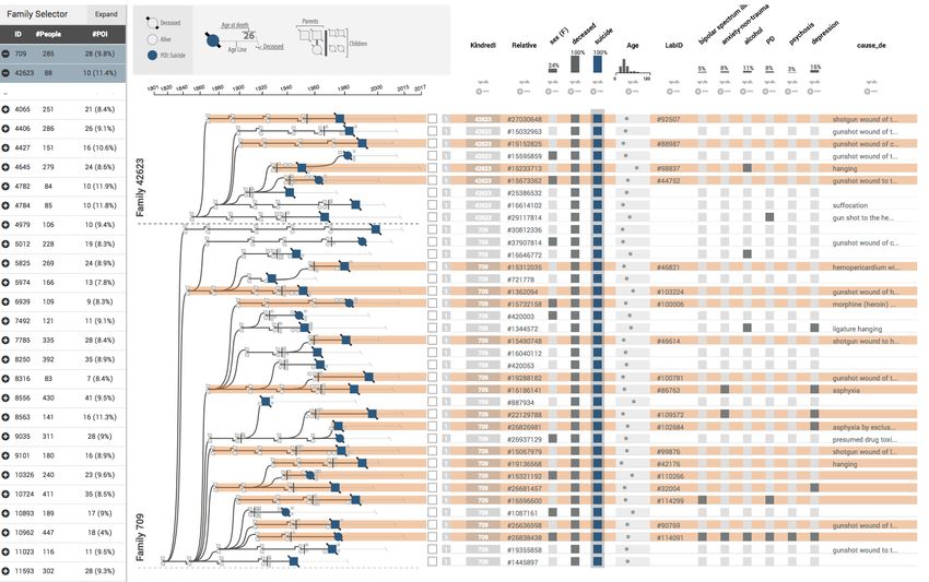
4

 T2 Analyze individual case. Our collaborators need to investi-         graph visualization techniques are optimized for either topology
    gate the context of a case. For example, a potential genetic        or attribute-based tasks [72], yet in many applications topology
    component contributing to suicide is judged differently if the      and attributes have to be judged in concert [59]. When analyzing
    person had many psychiatric comorbidities and committed             genealogies, for example, our collaborators want to understand how
    suicide at a young age, compared to a late-life suicide of a        two people with a similar phenotype are related, requiring them to
    person with a terminal disease.                                     first identify the phenotypes using the attributes, and then to judge
                                                                        their relatedness using the topology of the genealogy.
 T3 Compare cases. This task encompasses comparing indi-
    viduals and identifying shared attributes to characterize a              Partl et al. [59] classify four basic approaches to visualize
                                                                        multivariate networks for explicit graph layouts: (1) on-node
    potentially meaningful shared phenotype. It also pertains to
    analyzing how the individuals are related, which can indicate       mapping, i.e., visualizing the attributes by changing a visual
    the likelihood of shared genetic traits. Insights on shared         channel of the node mark or by embedding a small visualization in
                                                                        the node; (2) small multiples, i.e., showing the same graph multiple
    environmental factors can be gleaned from both the family
                                                                        times and visualizing a different attribute on top of each small
    structure and the attributes. For example, siblings are likely
                                                                        network; (3) separate, linked views for the graph and the attributes;
    to be exposed to the same environment in their childhood,
                                                                        and (4) adapting the graph layout to better fit the needs of attribute
    whereas cousins might not. Similarly, two people living in the
                                                                        visualization.
    same area are potentially of similar socioeconomic status.
                                                                             These approaches have different strengths and weaknesses with
 T4 Judge prevalence and clusters of phenotype. The number              respect to the tasks they enable. Lee et al. [41] distinguish, among
    of suicide cases and the prevalence of comorbidities vary           others, topology-based tasks, i.e., tasks that are related to the
    greatly between families and between branches of a single           network’s connectivity, and attribute-based tasks, i.e., tasks that are
    family. Judging how common a phenotype is in a family or in         related to the attributes associated with the nodes.
    part of the family is helpful in identifying subsets of interest         Although on-node mapping simultaneously supports topology
    for further study.                                                  and attribute-based tasks, it does so for only a few attributes because
 T5 Compare families. Once an interesting observation has been          the node size limits how many attributes can be encoded. Also,
    made in one family, our collaborators want to be able to            on-node visualizations are typically not aligned and have distractors
    investigate whether similar cases also appear in other families.    between them, which makes accurate comparison difficult [13].
    For example, when an association of asthma with suicide is          Gehlenborg et al. [22] review multiple systems that use on-
    discovered, they want to know whether it is isolated in one         node mapping for biological networks. An example for slightly
    family or occurs in multiple families and/or individuals.           more complex visualizations embedded on nodes is the Network
                                                                        Lens [29]. The work by van den Elzen and van Wijk [72] is a
 T6 Quality control. Although not an analysis task per se, our          special case of an on-node mapping approach: instead of mapping
    collaborators also need to judge the quality of the data and        data directly onto nodes in the networks, they aggregate nodes
    report errors back to the central database. A common data           into supernodes, show the relationships between the supernodes,
    error we have seen is disconnected components or detached           and visualize the attributes of these nodes in small, embedded
    nodes, which are caused by missing information about an             visualizations.
    individual’s mother or father.                                           Small multiples are also commonly used to visualize attributes
    Most of these domain tasks rely on both studying the topology       on top of graphs. Barsky et al. [5] and Lex et al. [44], for
of the network, i.e., the family relationships, and investigating       example, use small multiples to show gene expression data on
the attributes associated with the individuals. For example, the        top of biological networks. Using small multiples for multivariate
“compare cases” task (T3) relies on both the graph and the attributes   networks, however, has the disadvantage that the individual
to, for example, reject an outlier in an otherwise well-defined         networks have to be rendered in less space, limiting their readability
phenotype within a family, if that outlier is only distantly related    or the size of the graph for which they are useful.
to other cases.                                                              Separate, linked views excel at visualizing the attributes and
                                                                        the graph individually, but do not support the integration of both
4     R ELATED W ORK                                                    well. Systems that use this approach [42], [66] rely on linking
                                                                        and brushing to associate a node with the representation of its
We focus our discussion of previous work on specialized genealogy
                                                                        attribute, which requires interaction to reveal relationships between
visualization tools and on multivariate network visualization,
                                                                        the topology and attributes.
since genealogies are highly multivariate graphs. With regard to
                                                                             The fourth approach to multivariate graph visualization is
multivariate network visualization approaches, we also restrict
                                                                        to adapt the layout of the network so that the nodes can be
our discussion to explicit layouts (i.e., node link layouts) because
                                                                        easily associated with an effective attribute visualization. This
implicit layouts (such as SunBursts and treemaps) are ill suited
                                                                        approach is taken to the extreme in GraphDice [9], where nodes
to visualize attributes at all levels of the hierarchy; and matrices
                                                                        are positioned in a series of scatterplots based only on attribute
are not an ideal choice for genealogies since (1) the nodes are
                                                                        values. Less extreme approaches are various linearization strategies
only sparsely connected, hence wasting space, and (2) matrices
                                                                        where graphs are laid out such that associated attributes can be
are ill suited for path tracing, which is a common task of our
                                                                        visualized in efficient tabular layouts, overcoming the drawbacks
collaborators.
                                                                        of completely separated linked views. Typically, trade-offs for
                                                                        optimizing the readability of the topology or the linear layout have
4.1   Multivariate Networks                                             to be made. Meyer et al. [52] manually linearize a complete network
A multivariate network is a graph where the nodes and the               and render attributes next to the linear layout. This approach is
edges are associated with potentially rich attributes [32]. Many        efficient, but the complexity of the networks for which it is feasible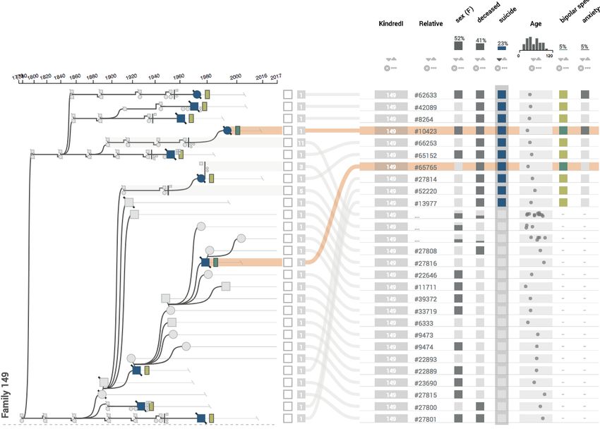
5

is limited, and topological structures can be hard to see. Partl et       drawing tool that closely follows the standard for visualizing
al. [59] use interaction to extract paths from a network, linearize       genealogies [6], [7]. (See the supplementary material for an
these paths, and associate the nodes in the paths with rows in a          example figure created with Progeny.) Although Progeny is well
tabular visualization. This approach, however, requires interaction       suited to draw these standard genealogies for use in presentations,
and works only for selected subsets of the graph. The recently            it is ill suited for exploratory tasks, mainly because of its inability
published Pathfinder system [58] uses path queries on networks            to efficiently encode attributes in the graph.
and presents the resulting paths in a linear, ranked list, juxtaposed          Interactive genealogy visualization tools that are designed to
with rich attribute data. This approach, however, is sensible only        analyze disease clusters and to see disease propagation within
for tasks related to paths.                                               families include PedVizApi [19], CraneFoot [46], Haploview
     Our work falls into the category of adapting the layout by           [4], PediMap [73], and HaploPainter [70]. HaploPainter [70]
linearization. We leverage the fact that the genealogical graphs          visualizes genealogies and genetic recombination events below
our collaborators are interested in are tree-like and linearize the       the individuals’ nodes. Although it shares the approach of showing
positioning of the nodes in the tree. We use this tree to juxtapose       metadata as rows associated with nodes with Lineage, it does
scalable and perceptually efficient visualizations of the attributes.     not take a linearization approach to make values of different
                                                                          generations easy to compare, it does not aggregate the network,
4.2   Tree Visualization                                                  and it does not visualize different types of attributes. McGuffin
                                                                          and Balakrishnan [50] describe layout algorithms for complicated
Many examples of multivariate tree visualization techniques are
                                                                          genealogical trees and introduce aggregation methods for subtrees,
available, yet none scale to more than a handful of attributes
                                                                          which we adopt.
and work for both intermediate nodes and leaves at the same
                                                                               Among tools that do not use the standard genealogical drawing
time. The on-node mapping strategies discussed in the previous
                                                                          conventions are Fan Charts [15], which uses the SunBurst technique
section can also be applied to visualizations of trees (e.g., [12]),
                                                                          to visualize genealogical trees, and the work by Mazeikla et
with the same limitations with respect to scalability. A common
                                                                          al. [49], which employs a force-directed layout that considers
example for tree visualizations associated with many attributes is
                                                                          similar phenotypes as additional attracting forces. Tuttle et al. [71]
the use of a dendrogram tree derived from a hierarchical clustering
                                                                          use an H-tree layout for scalable genealogy visualization, with
algorithm that is aligned to a heat map [16], [43], [65]. Similarly,
                                                                          the founder at the center and successive generations radiating
the leaves of evolutionary trees can be aligned to heat maps of
                                                                          out based on a fractal pattern. Ball [3] employs the idea to not
the species’ traits [38], [39]. Engel et al. [17] use clustering
                                                                          represent generations as discrete units but use time to position the
to decompose a multidimensional dataset and represent it as a
                                                                          nodes, and also to draw a person’s life span. Kim et al. introduce
Structural Decomposition Tree. This approach is unique since it
                                                                          TimeNets [34], a technique also focused on the temporal aspects of
directly embeds a tree into a projection of a high-dimensional
                                                                          a genealogy. Although TimeNets is well suited to observe temporal
dataset, foregoing a tabular layout for the attributes. Also related
                                                                          changes in relationships between individuals, relationships between
to our approach are tree tables, since they can be found in file
                                                                          generations are harder to trace. The recent work by Fu et al. [18]
browsers, where the tree represents the structure of folder and files,
                                                                          focuses on visualizing the distribution of tree structures in many
and attributes such as the file size are shown. Tree tables generally
                                                                          families. The tool combines a Sankey diagram showing properties
do not provide aggregation functionality — a branch can be either
                                                                          of tree structures with explicit node-link diagrams on demand, but
collapsed or expanded, but cannot be aggregated.
                                                                          does not consider attributes of the nodes.
    Implicit tree visualization techniques such as tree maps [28],
                                                                               GenealogyVis [45] is a recent tool for visualizing genealogies
sun burst [69], or icicle plots [36] are well suited to visualize one
                                                                          to study historic data. Although it visualizes multivariate attributes,
or two attributes of nodes in trees (using size and color), but they
                                                                          it addresses different needs — those of historians — and uses
do not scale to more attributes.
                                                                          different approaches. Unlike in Lineage, attributes of individuals
    These approaches either scale to many attributes for the leaves
                                                                          are not shown; rather, the focus is on demographic trends in (parts
of large trees, or are limited to a handful of attributes for all nodes
                                                                          of) the network. Supplementary views, such as scatterplots and
of the tree. We are not aware of prior tree visualization approaches
                                                                          maps, allow historians to study, for example, migration patterns.
that also show rich attributes for intermediate nodes, either in
                                                                               Genealogy visualization tools for animal genealogies face a
aggregated form or for each node individually.
                                                                          different set of challenges compared to those for human genealo-
    Our approach is also related to tree visualization techniques that
                                                                          gies, as the number of descendants sired by individual animals
provide dynamic aggregation, since we aggregate branches of trees
                                                                          can be large, and complex interbreeding is common. Consequently,
to highlight nodes of interest. Our approach is based on the concept
                                                                          tree-based approaches are not well suited for these genealogies.
of degrees-of-interest functions [20], which is widely applied in
                                                                          Examples include CoVE [11] and VIPER [60]. VIPER introduces
trees [12], [27], including in the original paper, but is also related
                                                                          a sandwich view that CoVE also adopts. The sandwich view scales
to other focus+context tree visualization approaches [55]. For a
                                                                          well to many descendants of an individual, but only explicitly
broad overview of other tree visualization techniques, we refer to
                                                                          encodes the relationships between parents and their children.
the tree visualization reference by Schulz [63].
                                                                          More distant relationships can be revealed through highlighting.
                                                                          Helium [67] is a visualization technique for plant genealogies,
4.3   Genealogy Visualization                                             which commonly have complex crossing. It uses color coding and
Genealogical charts, as shown in Figure 2, are widely used in             scaling of nodes to encode up to two attributes.
genetic counseling and the literature on genetic diseases. They are            GeneaQuilts [10] is a matrix-based technique where each row
well suited to visualize a single phenotype of interest, but they         constitutes a person and each column a nuclear family. In early
are not suitable to map a complex phenotype to the node. Our              stages of our design process, we considered using a GeneaQuilt
collaborators currently use Progeny [62], a commercial genealogy          instead of our node link design, since GeneaQuilts produces a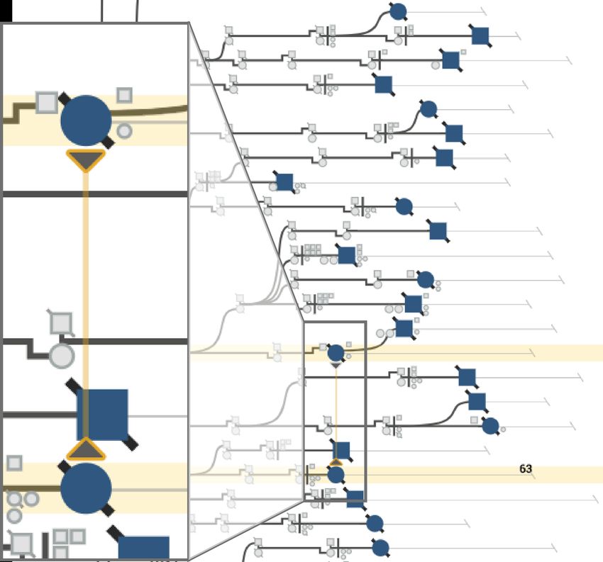
6

linearization of the graph that would be suitable for associating                                                            8
attributes. We ultimately decided against it because (1) the data we                                                    4
                                                                                     4    8           4    8
consider for the analysis of genetic relationship is predominantly                                                               *
                                                                                                                             7
tree-like, and hence, the complex design of GeneaQuilts that is                                                *        3
                                                                               1     3           1    3    7
necessary to accommodate general genealogical graphs is not                                                                  7*
                                                                                          7*               7*
justified for our simpler, tree-like datasets; (2) a key analysis task                                                       6
                                                                                     2    6           2    6
for the graph view is to judge the degree of relatedness between                                                             5
two nodes, which is not well supported by GeneaQuilts without                             5                5
                                                                                                                        2
interaction; and (3) our design for aggregation is more suitable for                                               1
node-link diagrams.
     A different approach to analyzing relatedness is to calculate                  (a)              (b)                     (c)
“kinship coefficients” between individuals, i.e., to calculate path-     Fig. 3. Decycling and linearization. (a) A directed, rooted graph with
                                                                         one cycle ending in node 7. (b) We remove the cycle by duplicating the
based metrics for relatedness and visualize them in a matrix [33].       last node in the cycle (node 7). (c) The tree is linearized so that each
Although this approach is scalable, it is not suitable for reasoning     node is assigned a distinct row. Leaves are rendered above their parents.
about all patterns of inheritance.                                       This row-based, linear layout enables an unambiguous, position-based
                                                                         association with a table visualizing attributes.
     A related tool that is concerned with visualizing phenotypes of
patient cohorts is PhenoStacks by Glueck et al. [23]. PhenoStacks        Linearization
uses a tabular approach similar to what we use for our table.            In most tree layouts [1], associating the nodes with rows in a table
                                                                         by position is impossible. The tree in Figure 3(b) is compact, yet
                                                                         would require, for example, curved links to associate the nodes
                                                                         with a table row. To make this association between nodes and rows
5     V ISUALIZING A M ULTIVARIATE G RAPH
                                                                         of a table intuitive, we use a linearization strategy that assigns
The tasks our collaborators need to address rely heavily on both         every node a distinct vertical position (i.e., a “row”). The position
the familial information contained in the genealogy graph, i.e., the     of the node alone thus unambiguously associates the node with a
topology, and the myriad of attributes associated with individuals       row in a table (see Figure 3(c)). Note that although we assume a
(see Section 3). Of the strategies for linearization introduced in       left-to-right tree layout here, a top-to-bottom layout would work
Section 4.1, only the linearization method enables an integrated         equally well for associating a tree with table columns.
analysis of topology and attribute at the scale of attributes we are         Linearized tree layouts are based on tree traversal strategies.
interested in. However, none of the described linearization methods      Although various strategies, such as breadth-first (level-order) or
are suitable for the data and tasks of our collaborators. Here, we       in-order depth-first-search, are possible, we found that a preorder
introduce a linearization method for tree-like graphs. We define         depth-first-search works well for our purposes, since it results in a
tree-like graphs as rooted, directed graphs that contain cycles. The     crossing-free layout and keeps leaves in subsequent rows.
purpose of the linearization is to associate the nodes with rows in a        Following the in-order strategy, we recursively place the
table visualization.                                                     descendants of a given node directly above their parents. Note
                                                                         that a top-down strategy would also be possible. We assume that
    A consequence of the linearization strategy is that the layout is
                                                                         an order of leaves can be defined, e.g., based on the attributes. If
not as compact as in other common layouts. To address this issue,
                                                                         not, using a random order is possible.
we also introduce degree-of-interest-based aggregation strategies
                                                                             Figure 3(c) illustrates the results of this algorithm when applied
that integrate seamlessly with the linearized graph.
                                                                         to the tree in Figure 3(b) and also shows how to easily associate a
    We illustrate this concept here using general, tree-like graphs,
                                                                         table with the tree. Note that the duplicate node also is duplicated
for now ignoring specific properties of genealogies. We later show
                                                                         in the associated table.
in Section 6 that this approach extends to genealogies (where each
person has two roots: their parents) with minor modifications, and       5.2       Aggregation
also elaborate on design decisions we made that are specific to our      Although linearizing the tree allows for a direct, position-based
data and application area.                                               association of the nodes and their attributes, the resulting layout
                                                                         uses more space than a compact layout. However, due to their
                                                                         hierarchical structure, trees are well suited for aggregation. Degree-
5.1   Linearization Approach                                             of-interest (DOI) functions [20] have been widely applied to trees.
                                                                         In our design, we use the generalized idea of degree-of-interest
De-Cycling
                                                                         functions by Furnas [20], [21].
In the first step, we remove cycles from the directed graph,                  We let analysts define a degree-of-interest function based on the
transforming it into a tree, by duplicating the node that completes      attributes of the nodes, which we call the phenotype of interest
a cycle, similar to the approach of Mäkinen et al. [46]. If the         (POI). Nodes that have the POI are referred to as nodes of interest.
duplicated node has children, we attach all children to one instance,    In contrast to the original formulation of a degree of interest, our
while the other instance remains a leaf. Figure 3(a) shows a tree-       POI function is binary (i.e., a node is either of interest or not) and
like graph with one cycle, Figure 3(b) shows the resulting tree,         does not consider a distance to a selected node. An example for a
where node 7 is duplicated. Although this duplication strategy           POI is “committed suicide”, which marks all nodes representing
works for general directed graphs, it is most useful for directed        individuals who committed suicide to be of interest, or “has a
graphs with a defined root and few cycles, since in these cases most     maximum BMI of higher than 30”, which would consider all obese
of the topology is retained, and the number of additional nodes is       individuals to be of interest. POIs that are a compound of multiple
negligible with respect to scalability.                                  attributes (high BMI and suicide) are possible.
7

                                                                                  The result in the associated table visualization is that each
         4   8

                                                                              node of interest has a separate row, and the aggregated branches
             7*
                                                                              are represented in aggregated rows. In practice, we use visual
         3                                    4   8                           encodings for aggregates and individual rows that can faithfully
                                                  7*                          represent the data but are also comparable. For details on the table
                  6                           3
                                                                              design, see Section 6.2.
             7*                                   7*
  1      2   5                         1      2   5     6
                                                                              Attribute-Hiding Aggregation
                  (a)                                  (b)                    This form of aggregation also preserves the complete structure of
Fig. 4. Aggregation approaches demonstrated using the tree in Fig-            the tree, but it does not preserve attributes of nodes that are not of
ure 3(c). A filled-in circle indicates a node of interest. (a) Attribute-     interest. The result, illustrated in Figure 4(b), is a scalable approach
preserving aggregation. Each node of interest (shown in black) is in
a separate row. Branches without nodes of interest are aggregated into        that can be used to address tasks that are concerned only with the
one row, yet all attributes are preserved in the aggregate representations    attributes of the nodes of interest and their connectivity, but not
in the table. Notice how the two children of node 2 who are not affected      with the attributes of the other nodes.
are shown using an implicit encoding, which we refer to as a “kid grid”.
(b) Attribute-hiding aggregation. The branches leading to nodes of interest
                                                                                  The main difference compared to the attribute-preserving
are hidden behind them. Only nodes of interest and branches with no           aggregation is that nodes of interest are not assigned to a new
nodes of interest have a row of their own. Only the nodes of interest are     row when they are encountered. The algorithm again recursively
represented in the table.                                                     follows a (sub)tree down a branch by assigning a new row to
    Based on this degree-of-interest function, we introduce two               each inner branch. If no nodes of interest are encountered while
approaches to aggregation that vary in how they trade off compact-            traversing the branch, the leaves are placed in a kid grid. If a node
ness and preservation of the attributes of the nodes: (1) attribute-          of interest is encountered, the next step depends on whether it has
preserving aggregation, and (2) attribute-hiding aggregation. These           children that are inner nodes or not. For the node’s children that
aggregation approaches can, of course, be applied not only to the             are leaves, a kid grid is used, but no new row is started. For all
whole tree, but also to selected subtrees, or to both.                        other branches, the algorithm is applied recursively.
                                                                                  The resulting layout has M rows, where M is the sum of:
Attribute-Preserving Aggregation                                                 • the number of inner branches,
Here we introduce an aggregation strategy for linearized layouts                 • the number of nodes of interest that have at least one child
that preserves both the structure of the tree and the attributes of                 that is an inner node.
all the nodes. Nodes of interest are assigned a row of their own,                 Here, only nodes of interest and inner branches that do not end
whereas other nodes are aggregated into a single row. Figure 4(a)             in a node of interest are assigned their own row. For consistency,
shows an example of this strategy applied to the tree shown in                we do not represent branches that do not end in a node of interest
Figure 3(c). This layout emphasizes the nodes of interest, while              in the table.
preserving both the structure of the graph and the attributes of the
other nodes.
     Our algorithm recursively follows a (sub)tree down a branch              6     L INEAGE D ESIGN
by assigning a new row to each inner branch. Inner branches are               Here we describe the design decisions that are specific to the use
branches that do not end in a leaf after the first edge, i.e., an edge        case of visualizing genealogies and that we realized in the Lineage
that directly connects to a leaf is not an inner branch. If no node           prototype. To address the tasks of our collaborators, Lineage
of interest is encountered, the algorithm continues to the leaves,            provides three views, shown in Figure 1: the genealogy graph
placing all nodes of the branch in the same row. Multiple leaves              view, the closely synchronized table view, and a family selection
that are not of interest are placed in a kid grid, an implicit encoding       view, which allows analysts to select one or multiple families.
of the leaves as small nodes to the right of their parent. These nodes
retain all visual encodings (e.g., shape for gender, crossed-out for          6.1   Genealogy Graph
deceased). We chose this approach for the representation of kid               An important difference between genealogical trees and general
grids over alternative designs such as a numeric labels or bar charts         trees is that nodes have not one but two parents. To address this, we
since it is consistent with how individuals are represented in other          introduce the concept of a couple, indicated by a line connecting
places in the tree. An example is visible in the bottom branch in             the partners (see Figure 5(a)). As is common in genealogical
Figure 4(a), where nodes 1, 2, 5, and 7 are on the same row, and the          graph layouts, the children of a relationship then connect to the
leaves (5, 7) are in a kid grid. If a node of interest is encountered,        line representing the couple instead of directly to the parents.
we distinguish two cases. If the node of interest has children that           We also adopt some of the conventions for drawing genealogical
are leaves and that are not nodes of interest themselves, they are            graphs: males are drawn as rectangles, females as circles. Deceased
added to a kid grid, which is placed in the next row (see node of             individuals are crossed out. In Figure 7(b), for example, the topmost
interest 3,) and its descendant (node 7), which is placed in a kid            node represents a female who is alive and has the POI, but the other
grid in Figure 4(a)). If the node has children that are inner nodes,          nodes with the POI are deceased. Nodes that have the phenotype
the algorithm is applied recursively. The result of this algorithm is         of interest are filled in.
a layout that has N rows, where N is the sum of:                                  As discussed in the previous section, the phenotype of interest
   • the number of nodes of interest,                                         can be defined dynamically, based on either combining categorical
   • the number of inner branches that do not end in nodes of                 values or brushing a range of a numerical variable. Figure 7 shows
      interest (case for node 4 in Figure 4(a)),                              the effect of two different POI functions on the same subtree.
   • the number of nodes of interest that have children that are                  The modifications to the layout algorithm to accommodate
      leaves (case for the child of node 3 in Figure 4(a)).                   couples are minor: couples are always placed in consecutive rows
8
6.1.1 Aggregation Layouts
With respect to aggregation, the algorithm is extended only by first
looking for spouses before descending into a subtree. If both are
nodes of interest, each spouse is assigned his or her own row.
(b) Aggregated layout We previously introduced the concept of kid grids for ag-
gregated nodes. Indicating hidden nodes using a glyph has been
done before for graph layouts, most notably by McGuffin and
Balakrishnan [50], who use dots to indicate children in genealogical
(c) Hidden layout
graphs. Our layout for aggregated genealogies, however, goes
beyond a basic indication of existing nodes as they encode both
topological information and attributes. First, we extend the notion
(a) Expanded layout of a kid grid that encodes children to a family grid that encodes
all members of a family. Figure 5 shows multiple examples. A
(d) (e) family is separated by a vertical line into parents and children. This
Fig. 5. Different aggregation cases. (a-c) A family where one woman vertical line represents the line used to connect spouses in expanded
has children with two men. One of the children committed suicide. (a) mode. Parents are placed on the left of the line. In addition to the
No aggregation: every person is in his or her own row. (b) Attribute
aggregation: the suicide case is in its own row; the rest of the family is node shape, we also redundantly encode sex by position, placing
aggregated. Notice the family grid with two male and one female parents, the nodes representing males on top and the nodes representing
and one daughter and one son. The second son is not in the kid grid females below. In families with multiple partners, we place all
because he is a node of interest. (c) Attribute hiding: the family is hidden
behind the suicide case. Only the attributes of the suicide case will be
partners in the same family grid, so that, for example, a family
shown in the table. (d-e) A different family, where the node of interest has with a woman who has children with three partners is represented
children, leading to special cases. (d) Attribute aggregation: the spouses by three squares on top and one circle at the bottom.
and children are moved to their own row. The line connecting spouses Note that aggregation results in some information loss. For
spans two rows. (e) Attribute hiding: the spouses are placed to the left of
the suicide case, the children to the right. families in which individuals have offspring with multiple partners,
the exact association between children and parents is lost. Also, the
to avoid long, vertical parent edges. When one of the spouses attributes for all aggregated nodes in a row are displayed together in
has offspring with multiple partners, we place all partners in the table, removing the exact association between individuals and
consecutive rows. In the case of two partners, we place the person their attributes; instead, the distribution of values in that aggregate
with multiple relationships in the center to avoid edge crossings. is emphasized. When hiding is used, the attributes are removed
Figure 5(a), for example, shows a woman who had children with entirely from the table. We found that neither of these drawbacks
two partners. For more than two spouses, however, or spouses is a problem since these design decisions align with the analysis
who had children with different partners in alternating order, edge tasks outlined earlier: analysts at first are often interested in nodes
crossings are often unavoidable. Similar to Mäkinen et al. [46], with the POI. When they want to consider other nodes in detail,
we use arrows to indicate that a node is duplicated and to point they can deaggregate on demand.
toward the duplicate. To resolve any ambiguities, we draw an
It is important to note that we break with the convention of
edge connecting the duplicates when hovering over the arrow (see
placing nodes based on their birth-year for aggregated families.
Figure 6).
Instead, we place the whole family based on the birth year of the
In contrast to traditional genealogical graphs, we do not lay parent with a blood relationships to the ancestors.
the nodes out by generation, but use the birth year to position the
nodes horizontally [3], as shown in Figure 1. This approach avoids
6.1.2 Encoding Attributes in the Graph
ambiguities about the birth order and encodes a vital attribute
directly in the graph. We also use curved splines instead of the Although we address the problem of encoding multiple attributes
traditional orthogonal edge routing, because continuous edges are for nodes using our linearization approach, direct, on-node encod-
easier to follow [75]. ing of a small number of attributes provides the best bridge between
attribute-based and topology-based tasks. We already discussed
how sex (shape), deceased/alive (crossed out), birth year (horizontal
position), and POI (fill) are encoded directly in the graph. To enable
our collaborators to view an additional variable in the graph, we
introduce a glyph, rendered to the right of the nodes, as shown in
Figure 8. When the attribute is categorical, we color-code the glyph;
for numerical attributes, we show a small bar. In both cases, the
color coding is also used in the table to highlight the relationship
(see the matching colors for bipolar disorder in Figures 8(a) and 9).
When data is not available for a node, no glyph is shown.
Finally, we also encode the age of individuals directly in the
graph by drawing a line from the node, which is placed at the year
of birth, to the year of death, or to the current year (see Figure 8).
These age lines conveniently encode an important variable in the
Fig. 6. Visual encoding of nodes that were duplicated in the process of
removing cycles from the graph. The arrow glyph, which is shown at all existing coordinate system. We found that the age lines also help
times, indicates both the presence of a duplicate and its direction in the to perceptually connect the nodes to the rows in the table. Since
graph. Hovering over the arrow draws a line connecting the node to its we do not draw age lines for aggregates, we found it necessary to
duplicate and highlights the corresponding rows in the table.9
(a) POI: Suicide (b) POI: Age < 40
Fig. 7. Different POI functions applied to the same aggregated subtree.
(a) Suicide as a categorical POI. (b) Age < 40 as a numerical POI.
Fig. 10. The table is sorted by suicide, which causes the rows in the table
to be in a different order than the rows in the graph. The association
(a) Categorical attribute (b) Numerical attribute between the two is retained by the curves connecting them.
Fig. 8. Attributes encoded directly in the graph. Age lines visualize the categorical values as stacked bars, which are scaled according to
lifespan of individuals. Age lines for people who are alive continue until
the present. Age lines of deceased individuals are terminated at their the number of individuals in a category. Text labels and IDs do not
year of death. We can see that the individual represented by the node of have adequate visual representations for groups of elements, so we
interest died at age 31, and his spouse died shortly thereafter. Selected display an ellipsis (...) for aggregates. Missing values are rendered
attributes can be visualized next to the nodes in glyphs (green rectangles). as a dash to distinguish them from zero or false values. We also
(a) The categorical variable bipolar disorder is encoded by a dark-green
color. (b) The numerical variable number of bipolar diagnoses is encoded provide a column that shows how many people are in a given row.
as a bar chart. We avoid color to encode data, so we can employ it to highlight
indicate the connection to the table using a light-gray background, elements of interest, such as to highlight selected rows and to
as can be seen, for example, in Figure 7. indicate the column that encodes the user-selected phenotype of
interest and the primary attribute. In Figure 9, the selected attribute
(bipolar) and the POI (suicide) are rendered in color. A menu in
6.2 Table Visualization the columns allows analysts to set the POI, set an attribute as a
The attribute table is designed to visualize both rows representing primary attribute, and star an attribute. Starring an attribute adds it
individuals and aggregates representing multiple individuals in the to the family selector table.
same space. The attributes visualized in the table can be chosen These features, in combination with the graph, allow analysts
using the Table Attributes menu in the tool bar. As shown in to address the tasks related to analyzing individuals (T2) and
Figure 9, we use dot plots to encode numerical data. Combined comparing cases (T3).
with transparency and jitter, dot plots can also be used to encode Finally, we also allow analysts to sort the table based on
aggregate rows. For categorical values, we distinguish between any column, which enables them to to easily identify clusters of
binary categories, such as deceased or alive, and multivalued similar items (T4). However, sorting by attribute removes the close
categories, such as race. We encode binary categories in a single association with the graph. To partially remedy this problem, we
column, as can be seen for “sex (F)”, where a dark cell corresponds draw slope charts, similar to what is used in LineUp [26], to relate
to true and a light cell corresponds to false. For multivalued the rows of the table to the rows of the graph. These connection
categories, we use a method commonly employed by Bertin [8], lines work well for a small number of rows, but often result in
and use one binary column for each category instead of, e.g., using significant crossings when dealing with many rows. In that case,
color to encode categories. We represent aggregates of binary or interactive highlighting helps to trace the lines. Lines that end in
an off-screen location are not rendered. Instead, an icon indicates
the direction of their corresponding row. Clicking on the icons
automatically scrolls to the location of the corresponding row in
the table. Figure 10 shows an example of a partially aggregated
graph sorted by suicide.
6.3 Viewing Multiple Families
One important aspect of our collaborators’ workflow is the compar-
ison of multiple families (T5). A requirement for comparison of
families is the ability to select families T1, which is enabled by the
Fig. 9. The table view. The first column encodes how many individ-
family selection view, shown on the left in Figure 1. The family
uals are aggregated in that row. Binary categories are represented selection view shows statistics about the family, such as its size, the
as present/absent (e.g., sex). Aggregates of binary variables show number of people with the currently selected POI, and the number
the proportions of the variable in stacked bars. Numerical values are of people who have a starred attribute. Combined with sorting, this
encoded using dot plots, which are also used for aggregates. The POI is
highlighted using a gray background. The depression column is starred, feature is useful to identify families with a high incidence of an
also indicated by the gray background.10
attribute, for example, to identify families in which bipolar disorder 8.1 Prioritizing Families for Analysis
is common. Multiple families are seamlessly integrated into the Dr. Coon uses the suicide dataset described in Section 2 for her
graph and table views (see Figure 11). To visually separate the analysis. Using established familial relative risk methods [31], she
families, a dashed line is drawn between them. ascertains a large number (>200) of extended multigeneration
high-risk families for analysis [14]. Limited time for analysis
and resources requires her to prioritize these families based on
7 I MPLEMENTATION AND P REPROCESSING data visualized in Lineage. Our collaborator’s goal is to select
a promising family for the computationally expensive analysis
Lineage is open source, is implemented in TypeScript as a Caleydo of Shared Genomic Segments (SGS) [74]. SGS investigates the
Phovea client/server application [25], and uses D3 for rendering. significance of genomic segments shared between distantly related
The server component is based on Flask and is provided as a affected cases. If an observed shared segment of the genome is
Docker container for easy deployment. A prototype of Lineage significantly longer than expected by chance, then inherited sharing
is available at https://lineage.caleydoapp.org. The source code is is implied. A greater distance separating cases (i.e., path-distance
available at https://github.com/caleydo/lineage. in the genealogy graph) translates to the increased statistical power
The prototype made available publicly contains 10 selected and of the method: chance inherited sharing in distant relatives is
anonymized families from the suicide study based on data from improbable. Finding cases with shared sequences that also have
the Utah Population Database. The anonymization method and a shared phenotype (suicide, plus potentially other comorbidities)
the selection of families were approved by the Utah Resource for allows Dr. Coon to reason that the sequence is a factor in these
Genetic and Epidemiologic Research (RGE). The anonymization phenotypes.
process involves randomizing the sex of individuals and the birth Previous analyses exploring the statistical power of SGS using
and death years and randomly deleting individuals, in addition to simulated high-risk families indicated that power is determined by
omitting attributes that could be identifiable. Hence, we do not familial distance (path length) between cases with genomic data
recommend making clinical inferences based on the data provided. for analysis, indexed by counting the total number of generations
separating the cases (meioses). In this study, if families had at least
15 meioses between cases, then 3-10 families were sufficient to
8 C ASE S TUDIES gain excellent power (>80%) to see at least one true positive within
any given family [35]. For all scenarios considered, genome-wide
We present two forms of validation for Lineage: case studies,
association studies (i.e., studies that do not consider familiarity)
a method employed widely to demonstrate the fitness for use
would have negligible power to detect the simulated variants. This
of visualization design studies [37], [64], and informal usability
study therefore dictated that extended high-risk families should be
testing and analyst feedback, which is described in the next section.
selected with the highest familial relative risk, and with the largest
The case studies outlined below were conducted with Dr. Hilary number of cases with genotyping available for analysis through
Coon, a psychiatry researcher and principal investigator studying interrogating numbers of cases with DNA, and familial distance
the genetic and environmental factors in suicide. Dr. Coon, who is of these cases from one another. Familial distance is visualized in
a coauthor of this paper, also participated in the analyst feedback the graph view in Lineage and serves as a useful predictor of the
sessions described in Section 9, and contributed to the design statistical significance of shared regions among cases. However,
and development of Lineage. She was familiar with the interface additional data about the cases shown in the table view of Lineage
from the earlier analyst feedback sessions as well as through is useful in later prioritization of genes in regions with significant
demonstrations during the design phase. For the case study, we evidence of sharing. These attributes include gender, young age at
deployed Lineage on a secure, password protected and HIPPA death, and clustering of comorbidities.
compliant server instance on Amazon Cloud Services, which Figure 11 shows two families of high interest (709, 42623),
allowed her to access the tool from her personal computer, in based on significant familial risk ratios (pYou can also read