Fast Gravitational Approach for Rigid Point Set Registration With Ordinary Differential Equations
←
→
Page content transcription
If your browser does not render page correctly, please read the page content below
Received April 26, 2021, accepted May 21, 2021, date of publication May 27, 2021, date of current version June 7, 2021.
Digital Object Identifier 10.1109/ACCESS.2021.3084505

Fast Gravitational Approach for Rigid Point Set
Registration With Ordinary Differential Equations
SK AZIZ ALI 1,2 , KEREM KAHRAMAN2 , CHRISTIAN THEOBALT                                                   3,

DIDIER STRICKER1,2 , AND VLADISLAV GOLYANIK3
1 Department of Computer Science, Technische Universität Kaiserslautern, 67663 Kaiserslautern, Germany
2 German Research Center for Artificial Intelligence GmbH (DFKI), Augmented Vision Group, 67663 Kaiserslautern, Germany
3 Max Planck Institute for Informatics, Saarland Informatics Campus, 66123 Saarbrücken, Germany

Corresponding authors: Sk Aziz Ali (sk_aziz.Ali@dfki.de) and Vladislav Golyanik (golyanik@mpi-inf.mpg.de)
This work was supported in part by the Project VIDETE through the German Federal Ministry of Education and Research
[Bundesministerium für Bildung und Forschung (BMBF)] under Grant 01IW18002, and in part by the European Research Council (ERC)
Consolidator Grant 4DReply under Grant 770784.

  ABSTRACT This article introduces a new physics-based method for rigid point set alignment called
  Fast Gravitational Approach (FGA). In FGA, the source and target point sets are interpreted as rigid
  particle swarms with masses interacting in a globally multiply-linked manner while moving in a simulated
  gravitational force field. The optimal alignment is obtained by explicit modeling of forces acting on the
  particles as well as their velocities and displacements with second-order ordinary differential equations of
  n-body motion. Additional alignment cues can be integrated into FGA through particle masses. We propose a
  smooth-particle mass function for point mass initialization, which improves robustness to noise and structural
  discontinuities. To avoid the quadratic complexity of all-to-all point interactions, we adapt a Barnes-Hut
  tree for accelerated force computation and achieve quasilinear complexity. We show that the new method
  class has characteristics not found in previous alignment methods such as efficient handling of partial
  overlaps, inhomogeneous sampling densities, and coping with large point clouds with reduced runtime
  compared to the state of the art. Experiments show that our method performs on par with or outperforms all
  compared competing deep-learning-based and general-purpose techniques (which do not take training data)
  in resolving transformations for LiDAR data and gains state-of-the-art accuracy and speed when coping with
  different data.

  INDEX TERMS Rigid point set alignment, gravitational approach, particle dynamics, smooth-particle
  masses, Barnes-Hut 2D -Tree.

I. INTRODUCTION                                                                                   The objective of pairwise RPSR is, given a pair of
Rigid point set registration (RPSR) is essential in many com-                                  unordered sets of points generally in 2D, 3D, or higher-
puter vision and computer graphics tasks such as camera pose                                   dimensional space, to find optimal rigid transformation
estimation [1], 3D reconstruction [2], CAD modeling, object                                    parameters (e.g., 6DOF in 3D, rotation R ∈ SO(3) and
tracking and simultaneous localization and mapping [3], [4]                                    translation t ∈ R3 ) aligning the template point set to
and autonomous vehicle control [5], to name a few. Sup-                                        the fixed reference point set. One of the earliest method
pose we would like to merge partial 3D scans obtained by                                       classes — iterative closest points (ICP) [6], [7] — is still
structured light into a single and complete 3D reconstruction                                  among the most widely-used techniques nowadays, due to
of a scene, identify a pre-defined pattern in the 3D data or                                   its simplicity and speed. In ICP, the problem of RPSR is
estimate the trajectory of the sensor delivering 3D point cloud                                converted to transformation estimation between points with
measurements. All of these tasks can be addressed by a robust                                  known point correspondences. In each iteration, correspon-
RPSR approach which can cope with partially overlapping                                        dences are selected according to the nearest neighbor rule.
and noisy data.                                                                                Nevertheless, ICP is not the ideal choice in many challenging
                                                                                               scenarios with noise, partial overlaps or missing entries in
   The associate editor coordinating the review of this manuscript and                         the data, due to its inherent sensitivity to all these disturbing
approving it for publication was Mingbo Zhao             .                                     effects and the deterministic correspondence selection rule.

                     This work is licensed under a Creative Commons Attribution 4.0 License. For more information, see https://creativecommons.org/licenses/by/4.0/
79060                                                                                                                                                                 VOLUME 9, 2021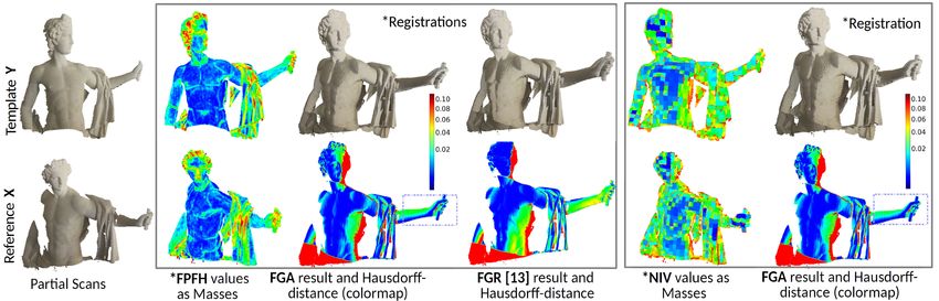
S. A. Ali et al.: Fast Gravitational Approach for Rigid Point Set Registration

FIGURE 1. A comparison between several standout rigid registration methods (state-of-the-art) on a randomly selected pair of low-overlapping point
clouds from popular 3DMatch [10] dataset. #Y and #X are the initial point sizes of the source and target scans. Due to the computational constraint,
the corresponding subsampled versions of the inputs (with point sizes #Yss and #Xss ) are used in the tests. The comparison shows alignment accuracy
as root mean squared error (RMSE) of distances between actual and transformed source, and runtime of each tested method. The RMSE metric, which is
              1 P#Y kR Y + t − R∗ Y − t∗ k2 )1/2 , defines the alignment accuracy based on the ground-truth transformation (R , t ) and estimated
mesured as ( #Y    i =1 gt         gt           2                                                                                    gt gt
transformation (R∗ , t∗ ). The red underline markers highlight the best case scenarios. Our method FGA is compuationally fast and robust compared to
GA [11], BHRGA [12], FGR [13], DGR [14], DCP-v2 [15], FilterReg [16], PointNetLK [17], Fast Robust ICP [18], point-to-point ICP [6], RANSAC [19],
GMMReg [20] and CPD [21].

To tackle these difficulties, many other techniques for RPSR                     techniques. Thus, automotive applications require real-time
were subsequently proposed over the last decades [8], [9].                       methods for aligning large, partially overlapping data with
   In recent times, RPSR methods relying on physical                             outliers and inhomogeneous point densities.
analogies [11], [12], [22], [23] are emerging. They offer an
                                                                                 A. CONTRIBUTIONS
alternative perspective to the problem and can often success-
fully handle cases which are difficult for other algorithmic                     In this article, we propose a new physics-inspired approach
classes. Physics-based methods have been successful in many                      to rigid point set alignment — Fast Gravitational Approach
domains of computer vision [24]–[26] and have multiple                           (FGA, Sec. IV) — which is our core contribution. In FGA,
advantages over other method classes. Moreover, by using                         point sets are interpreted are particle swarms with masses
physical principles, we have access to a large volume of                         moving under the simulated gravitational force field induced
research on computational physics. For instance, we can bor-                     by the reference as depicted in Fig. 1. The consecutive
row data structures and acceleration techniques which were                       states of the template are obtained by explicit modeling of
successfully applied in numerical simulations [27], [28].                        Newtonian particles dynamics and solving for displacements
   Although RPSR is a well-studied research area, we believe                     and velocities of the particles with second-order ordinary
that further advances are possible here with physics-based                       differential equations (ODEs). In contrast to methods based
techniques. With new sensors (e.g., LiDAR), the spatial prop-                    on correspondences selection and filtering [13], [19], [29],
erties like sampling accuracy and density or physical proper-                    FGA is a correspondence-free approach, i.e., its energy func-
ties like light-reflectance and color-consistency of the point                   tion is defined in terms of interactions between all template
clouds are considerable factors for the current alignment                        and reference points. Thus, our method is globally-multiply
                                                                                 linked and has properties not found in other related algorith-

VOLUME 9, 2021                                                                                                                                79061
S. A. Ali et al.: Fast Gravitational Approach for Rigid Point Set Registration
mic classes (e.g., high robustness to noise, versatile applica- competing methods, to the best of our knowledge, can-
bility of point masses and the fact that the locally-optimal not cope with such large data in such short time.
alignment is reached when the gravitational potential energy
of the system is locally-minimal). B. STRUCTURE OF THE ARTICLE
This article is partially based on our published confer- The rest of the article is organized as follows. In Sec. III,
ence paper [11], while featuring further contributions towards we first review the classical n-body problem and show how
the accuracy gain, computational complexity reduction, han- it can be adapted for RPSR. FGA is introduced in Sec. IV.
dling inhomogeneity in point clouds and feature-based We define our gravitational model with second-order ODEs
boundary conditions for tackling partially overlapping data. and simulation rules in Secs. IV-A–IV-E. Details on BH tree
To summarize: building and integration into FGA for accelerated alignment
can be found in Sec. IV-F. Embedding boundary conditions
• Besides the general settings of particle interactions through masses is elaborated in Sec. IV-G. FGA is then
and dynamics in [11] (Secs. IV-A–IV-D), we propose evaluated against multiple RPSR methods in Sec. V, followed
an acceleration technique with point clustering, i.e., by discussion and conclusive remarks.
Barnes-Hut (BH) tree [30] (Secs. IV-E–IV-F) which
II. RELATED WORK
reduces the algorithm’s quadratic computational com-
plexity to quasilinear. Especially for large point sets Related work on point set alignment is vast and can
as those arising in automotive and augmented reality be reviewed from different perspectives. We classify the
applications, FGA without acceleration can become pro- methods according to whether they alternate between
hibitive. Subsampling can alleviate the problem but the correspondence search and transformation estimation
leads to data loss (especially of high-frequency details) (Sec. II-A), rely on probabilistic modeling (Sec. II-B) of
as, ideally, one would like to use all available data. input data, are deep-learning-based (Sec. II-C) or are physics-
In contrast, our acceleration technique preserves the based (Sec. II-D).
explicit influence of all available data points as well as
the globally multiply-linked point interactions. A. FROM TRANSFORMATION ESTIMATION TO ICP
• Next, we show that particle masses in FGA can be Some approaches [13], [19], [29], [35] first extract a sparse
initialized using different types of boundary conditions set of descriptive key points from point sets [36], [37] and
such as prior correspondences and feature-based align- then find optimal alignment parameters with a transformation
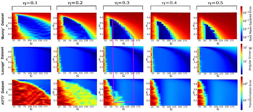
ment cues (Sec. IV-G). Thus, we propose a normal- estimation approach [38]–[42]. This policy does not use all
ized intrinsic volume (NIV) measure per point to be available points and often leads to coarse alignments but,
assigned as their mass. This is an effective weighting on the other hand, can result in a significantly improved ini-
scheme which smoothly balances the inhomogeneous tialization for other RPSR approaches [36]. Iterative Closest
point sampling density. Similarly, if some matches are Point (ICP), pioneered by Besl and McKay [6] as well as
given, radially symmetric weights can be assigned to Chen and Medioni [7], is an approach alternating between
the masses via a radial basis function (RBF) [31]. In the correspondence search and transformation estimation.
case of partially overlapping data with some known prior Various modifications of ICP have been introduced over
correspondences, the Hadamard product of RBF and the years [43]–[46] to tackle its local minima trapping issue.
NIV values as the assigned masses makes the method Segal and coworkers [47] extended the classical ICP with
robust and addresses the local minima issue. Other point probabilistic transformation estimation. In [9], a comprehen-
features like Fast Point Feature Histogram (FPFH) [19] sive overview of ICP variants is available.
are also adaptable for the point mass initialization.
• As it has been recently shown, resolving the uniform B. PROBABILISTIC METHODS
scale difference, i.e., the seventh DOF is not possi- Probabilistic approaches assign a probability of being
ble while using the globally multiply-linked interac- a valid correspondence to point pairs [20], [21], [48].
tion policy [32]. Thus, in 3D 6DOF pose estimation, Chui and Rangarajan [48] interpret point set alignment as
we perform an extensive evaluation of FGA against a mixture density estimation problem. Their Mixture Point
multiple widely-used and state-of-the-art rigid point Matching (MPM) approach iteratively updates probabilis-
set alignment methods and show applications of FGA tic correspondences and the transformation with annealing
to LiDAR-based odometry [33] and completions of and Expectation-Maximization (EM) schemes, respectively.
real RGB-D scans [34] (Sec. V). FGA outperforms Coherent Point Drift (CPD) [21] models the template as a
general-purpose RPSR methods in scenarios with large Gaussian Mixture Model (GMM) which is fit to the reference
amounts of noise and partial overlaps. We can cope interpreted as data points. FilterReg [16] pursues an alterna-
with large samples originating from the modern LiDAR tive approach, i.e., the reference induces a GMM. This results
sensors — containing ∼400k points each — and can in a simpler, faster and — in some scenarios — a more accu-
support point cloud based odometry at ∼1.5 pairs per rate algorithm compared to CPD. In contrast to [16], [21],
second with our GPU version of FGA. In contrast, other GMM Registration (GMMReg) [20] interprets both point
79062 VOLUME 9, 2021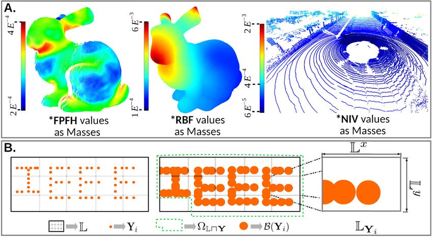
S. A. Ali et al.: Fast Gravitational Approach for Rigid Point Set Registration

sets as GMM, and point set alignment is posed as mixture                         interactions to quasilinear, and our parallelization on a GPU
density alignment. The approach of Tsin and Kanade [49]                          further lowers the runtime. At the same time, we obtain posi-
finds a configuration with the highest correlation between                       tional updates for particles by solving second-order ODEs.
point sets leading to the optimal alignment. Eckart et al. align                    BHRGA [12] is another gravitational approach for RPSR
inhomogeneous point clouds with hierarchical GMM [50].                           that modifies laws of gravitational attraction and converts
Several approaches additionally use alignment cues as prior                      it to non-linear least squares (NLLS) optimization problem
correspondences or colors of point clouds [51]–[54]. Our for-                    with globally multiply-linked point interactions [12]. Similar
mulation integrates prior correspondences and point features                     to our method, they also adapt a BH tree [30]. Relying on
by mapping them to point masses.                                                 a Gauss-Newton solver for NLLS has both advantages and
                                                                                 downsides. Even though [12] requires a smaller number of
C. DEEP LEARNING APPROACHES                                                      iterations until convergence on average compared to FGA,
Multiple techniques with deep neural networks (DNN) for                          our method enables fine-grained control over the paralleliza-
point cloud processing tasks (e.g., classification and segmen-                   tion and is tailored for a single GPU. We require ∼1 second
tation [55], [56] or shape matching [57]–[59]) have been                         for LiDAR data alignment, whereas BHRGA needs
recently proposed. RPSR approaches using DNNs have also                          ∼1.5 minutes [12] for the inputs of the same size, i.e., an
appeared recently in numbers [15], [17], [60]–[64]. Most of                      improvement of two orders of magnitude.
them [15], [17], [61], [62] utilize PointNet [55] as a deep                         In another physical interpretation, [71] solves small
feature extractor and feature matching layers for estimating                     correspondence problems on point sets using quantum
rigid transformations. In contrast, Deep Global Registration                     annealing [72].
(DGR) [14] — which is a data-driven version of Fast Global
Registration (FGR) [13] — uses 3D U-Net type feature                             III. N-BODY SIMULATIONS
extractors and a differentiable weighted Procrustes approach.                    The n-body problem is defined for a system of n astrophysical
   For all these DNN-based methods, the question of the                          particles in a state of dynamic equilibrium following New-
generalizability to point sets with arbitrary and different point                ton’s law of gravitational interactions [73]. For a two-body
cloud characteristics — such as point set density and volu-                      system, the total work done by the gravitational force of
metric sampling (e.g., in the case of a volumetric 3D scan                       attraction Fi by a stationary particle (at position rj with
of a human brain, in contrast to point sets representing sur-                    mass mj ) in bringing the other particle (at position ri with
faces) — remains open. We assume that no training data is                        mass mi ) towards it by displacing a distance of r units is
available and primarily (except for Sec. V-A) compare our                        defined            R r Gm m Potential Energy (GPE) Ei =
                                                                                    R r as the Gravitational
technique to the methods making the same assumptions.                            − rij Fi dr = − rij r 2i j dr. Analogously, for the case of
                                                                                 n particles the total GPE of an n-body system is defined as:
D. PHYSICS-BASED APPROACHES                                                                                n Z rj
                                                                                                          X       Gmi mj
Physics-based methods are also popular for many computer                                           E=−                    dr.              (1)
vision and graphics tasks. These methods interpret inputs                                                      ri    r2
                                                                                                              i,j=1
as physical quantities and transform the data according to                                                     i6 =j
physical laws [65]–[67]. Several algorithms from different                          The total gravitational force Fi exerted on the particle i by
domains of computational science use the law of universal                        the remaining n − 1 particles can be expressed as the sum of
gravitation [25], [26], [65], [66], [68]–[70].                                   the negative gradients of the total GPE φ(ri , t) and an external
   A modification of Wright’s gravitational clustering [65]                      potential φext [74]:
algorithm was used for image segmentation [24]. The method                                         n
                                                                                                   X         Gmi mj (ri − rj )
of Sun et al. for edge detection [66] — later improved                                Fi = −                                  3/2 −∇φext (ri ),     (2)
by Lopez-Molina et al. [69] — was shown to be more                                             j=1, j6 =i   kri − rj k2 +  2
robust in scenarios with noise, compared to several competing                                  |                 {z              }
                                                                                                              ∇φ(ri , t)
methods. A gravitational analogy was also applied in image
smoothing [70]. Recently, [25] proposed a weighting scheme                       where ∇ denotes the gradient operator and k·k denotes
with a gravitational model for stereo matching.                                  `2 -norm. The instantaneous system’s state is defined by
   Jauer et al. [23] developed a framework for RPSR based                        n position (ri ) and velocity (ṙi ) vectors at time t. The force
on the laws of mechanics and thermodynamics. Similarly                           softening parameter  helps to avoid degeneracy inside the
to our FGA, they model point clouds as rigid bodies of                           interaction region, i.e., when kri − rj k ≤ . Absence
particles and additionally support arbitrary driving forces                      of  also indicates collisional particle interactions. −∇φext
such as gravitational or electromagnetic, as well as repul-                      accounts for any probable external forces due to the friction or
sive forces. To reduce the runtime, they apply simulated                         other annealing factors in the system. This friction dissipates
annealing along with the Monte-Carlo re-sampling and cal-                        the fraction η of the particle momentum. After solving the
culate particle interactions in parallel on a GPU. This policy                   second-order ODEs of motion, the acceleration
does not improve upon the quadratic complexity. In con-                                                            Fi
trast, we reduce the computational complexity of particle                                                   r̈i =                              (3)
                                                                                                                   mi
VOLUME 9, 2021                                                                                                                                     79063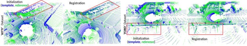
S. A. Ali et al.: Fast Gravitational Approach for Rigid Point Set Registration

provides the updated velocity
                         R         and displacement
                                        RR               as single      v) A collisionless n-body simulation is performed, since
and double integrals ( r̈i (t)dt and         r̈i (t)dt) over time,         the number of particles cannot be changed according to
and the trajectories of n particles are obtained in this phase             the problem definition;
space.1 The interactions between particles can either be colli-        vi) Astrophysical constants (e.g., G) are considered as
sional or collisionless. The total energy, kinetic and potential,          algorithm parameters;
of every particle is conserved for the collisionless interac-         vii) A portion of kinetic energy is dissipated and drained
tions or redistributed when collisions occur. The rules of                 from the system — the physical system is not isolated.
the energy exchange and altered kinematics in collisional
interactions [75] will force the particles to collapse and cause     B. GRAVITATIONAL POTENTIAL ENERGY (GPE) FUNCTION
topological degeneracy. For this reason, collisional dynamics        OF FGA
is beyond the scope of the RPSR problem domain.                      The locally-optimal rigid alignment is achieved at the sys-
                                                                     tem’s state with locally minimal GPE as shown in Fig. 2.
IV. THE PROPOSED APPROACH                                            If the system of particles Y moves as a rigid body, the optimal
This section describes our FGA with algorithmic steps on             alignment is achieved when the GPE between Y and X is min-
(i) how a constrained n-body simulation is fitted to define          imum. We solve the rigid transformation estimation problem,
the dynamics of the source object in Sec. IV-A, (ii) the             i.e., estimating rigid rotation R and translation t, applying
use of ODEs of dynamics to obtain minimum GPE for                    rigid body dynamics [76] on the displacement fields of the
locally-optimal alignment between the source and the target          points in Y. The GPE to rigidly move Y from its starting
in Secs. IV-B–IV-D, (iii) acceleration scheme for the whole          position towards X is expressed as a weighted sum of inverse
process of n-body simulation in Secs. IV-E–IV-F and, finally,        multiquadric functions on the distance fields:
(iv) defining boundary conditions for our energy function                                    X           mYi mXj
using mass initialization policies based on shape descriptors                 E(R, t) = −G                                 .     (4)
                                                                                                  (kRrYi + t − rXj k + )
in Sec. IV-G.                                                                                       i,j

A. NOTATIONS AND ASSUMPTIONS
In FGA, YM ×D = (Y1 . . . YM )T and XN ×D = (X1 . . . XN )T
are unordered sets of D-dimensional M template points and
N reference points, where Yi and Xj denote elements with
indices i and j from respective point sets. The following
parameters need to be set for n-body simulation which are
inherited in our FGA and explained in Sec. III:

    •   G — gravitational constant,
    •    — near field force softening length,
    •   η — constant system energy dissipation rate,
    •   1t — time integration step for the ODEs of motion,           FIGURE 2. GPE function plot with different optimization momenta
                                                                     handled by the increasing time differential (time step 1t ). Simulation
    •   mYi and mXj — point masses of Yi and Xj .                    steps depict the reference-template configuration at the current iteration.

   The proposed method considers the general settings for               Since the energy function in Eq. (4) is inverse multiquadric,
particle interactions from [11]. It takes X and Y as input           non-linear least-squares optimization methods do not fit. Also
sets of points and interprets them as (M + N )-body sys-             note, there exists a singularity (without ) at the optimal state
tem, where Y is optimally registered to X by estimating the          of Y as the distance field in the denominator approaches zero
rigid transformation tuple (R, t). For the registration pur-         (whereas E → −∞). We minimize (4) using second-order
pose, several assumptions and modifications are made for our         ODEs of motion for particle dynamics of Y, and iteratively
(M + N )-body system:                                                recover rigid transformations on its successive states.
    i) Every point represents a particle with a mass condensed
                                                                     C. ODEs OF PARTICLE MOTION (NEWTONIAN DYNAMICS)
       in an infinitely small volume;
   ii) A static reference X induces a constant inhomogeneous         The assumption (ii) constrains X to remain idle at a fixed
       gravitational force field and its points do not interact      position like a single body, formed by a set of non-interactive
       with each other;                                              points, which attracts Y. On the other hand, the assump-
  iii) Particles Yi move in the gravitational force field            tion (iii) allows every Yi to be attracted by X only. To this
       induced by all Xj and do not affect each other;               point, the dynamics of Y remains unconstrained, whereas
  iv) Y moves rigidly, i.e., the transformation of the template      relative positions of Yi will change at every time step. The
       particle system is described by the tuple (R, t);             momentum of Yi (from the intermediate previous state) will
                                                                     be preserved, and motion is tractable as the assumption (v)
  1 the space spanned by all possible particle states                restricts any form of merging or splitting of the points in Y.

79064                                                                                                                                  VOLUME 9, 2021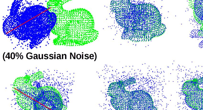
S. A. Ali et al.: Fast Gravitational Approach for Rigid Point Set Registration

Similar to Eq. (2), the gravitational force of attraction exerted                      rigid transformation between these two states, we solve the
on Yi by all the static particles from X reads as:                                     generalized orthogonal Procrustes alignment problem in the
                            N                                                          closed form.
                            X        mXj mYi (rYi − rXj )                                 Rotation Estimation: Given are point matrices Y and YD =
             FYi = −G                                             .              (5)
                                  (krYi − rXj k2 +  2 )3/2                            Y + D. Let µY and µYD be the mean vectors of Y and YD
                            j=1
                                                                                       respectively, let Ŷ = Y−1µTY and ŶD = YD −1µTYD be point
   Since gravitational force depends on the initial and final                          matrices centered at the origin of the coordinate system and
positions of a particle pair, it conserves the total mechanical                        let C = ŶTD Ŷ be a covariance matrix. Let USÛT be singular
energy of the system. The total energy conservation in our                             value decomposition of C. Then the optimal rotation matrix
case is analogous to preserve the momentum of Y only as X is                           R is given by [38], [41]:
static. The force from X, in Eq. (5), will bring the template
Y closer to its centroid and then Y will endlessly oscillate                               R = U6 ÛT , where 6 = diag(1, . . . , sgn(|UÛT |)). (15)
around that centroid. Modification (vii) allows for draining
                                                                                          Translation Estimation: Once the rotation R is resolved,
some energy in the form of heat as Y moves in a viscous
                                                                                       such that RŶ = ŶD , the current state of template point set
medium. We introduce a dissipative force FdYi :
                                                                                       can be updated as YD = RY + (1µTYD − R1µTY ) where the
                              FdYi = −η ṙYi ,                                   (6)   translation component is:

which is proportional to the particle velocity with the                                                     t = 1µTYD − R1µTY .                     (16)
factor η. It allows the otherwise endless periodic motion of the
template – due to second-order ODEs of motion – to settle.                             E. ACCELERATION POLICIES
Hence, the resultant force acting on every Yi is                                       Many acceleration policies can be used for n-body prob-
                                                                                       lems. Some studies show specialized hardware configura-
                            fYi = FYi + FdYi .                                   (7)   tions for massively parallel n-body simulations. GRAPE-4
  The next simulated state of Y at the time t +1t in the phase                         (GRAvity PipE) and GRAPE-6 [77] use pipelining of instruc-
space is obtained by estimating the unconstrained velocity                             tions in force computation and position update of particle set
                                                                                       sizes up to 104 and 106 , respectively. Logical parallelism of
                                                 f Yi                                  n-body simulation is also achieved on FPGA [78]. Few sem-
                        ṙt+1t
                          Yi   = ṙtYi + 1t           ,                          (8)
                                                 mYi                                   inal works have reduced the algorithmic complexity of the
and updating the previous rtYi with the displacement                                   n-body problem (e.g., Fast Multi-pole Method (FMM) [27]).
                                                                                       This runs the n-body algorithm in O(N log N ) time, but
                           dt+1t = 1t ṙt+1t                                     (9)   can also achieve O(N ) at the expense of higher force
                            Yi          Yi
                                                                                       approximation tolerance. It also has a relatively lower force
for all template points. The updated velocity and displace-                            approximation accuracy than BH method [30]. Although the
ment fields of the template points are stacked into matrices:                          runtime of FMM is similar to the BH method, we adapt the
           h                            iT                                             BH method because its underlying concept is simple and
     V = ṙt+1t
             Y1   ṙt+1t
                    Y2    . . . ṙ t+1t
                                   YM       (velocities),    (10)                      many astrophysical particle simulations using BH method are
           h                             iT                                            also successfully ported on FPGA and GPU [28], [79]. The
     D = dt+1t
             Y1 dY2
                     t+1t
                           . . . dt+1t
                                    YM       (displacements) (11)                      algorithmic steps of our RPSR method are not exactly the
and, similarly, the force residual and particle mass matrices:                         same as n-body algorithm. Hence, in this section, we show
                                T                                                     how BH tree can be applied to FGA. We are the first, to the
         F = fY1 fY2 . . . fYM

                                       (forces),          (12)                         best of our knowledge, to decompose the quadratic compu-
                                    T                                                 tational complexity of O(MN ) for all-to-all force computa-
       mX = mX1 mX2 . . . mXN

                                          (masses of X), (13)
                                    T                                                 tions to the quasilinear complexity of O(M log N ) using the
       mY = mY1 mY2 . . . mYM

                                          (masses of Y). (14)                          BH force approximation in a gravitational point set alignment
                                                                                       method with second-order ODEs.
D. RIGID BODY DYNAMICS USING ODEs OF MOTION
Newton-Euler equations of motion in mechanics (first, sec-                             F. BARNES-HUT FORCE APPROXIMATION
ond and third law of motion with Euler time integration) relate                        BH-tree-based force computation in FGA requires two
any external force f with the inertial state of the body. Newto-                       steps — BH tree construction and BH force calculation.
nian mechanics assumes an inertial frame of reference which                            BH Tree τ θ . The construction of τ θ is a method of hierarchi-
is fixed and excluded from any external force. According to                            cal space partitioning and grouping of particles as described
assumption (ii), the template and the reference are attached                           in Alg. 1 [30]. Given a system of particles with their known
to the moving body-fixed and the inertial frames of reference,                         position vectors, masses and dimensionality (D) as input,
respectively. After one step of our (M + N )-body simulation,                          this method at first constructs a tree structure of virtual
two states of the template are available — the previous state Y                        2D dimensional lattices, i.e., either cubical cells as nodes of an
and the current state Y + D. To recover a single consensus                             octree for 3D data or square cells as nodes of a quad-tree for

VOLUME 9, 2021                                                                                                                                     79065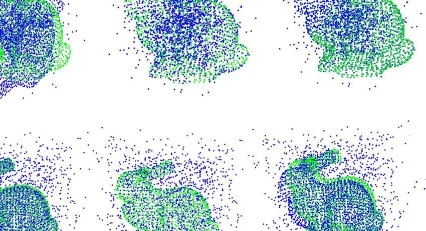
S. A. Ali et al.: Fast Gravitational Approach for Rigid Point Set Registration

2D data. To construct τ θ , the following steps are performed        Algorithm 1 Build BH Tree
iteratively until each particle is assigned to its leaf nodes:        Input: reference XN ×D , masses MX , maximum tree
   i) BH tree partition starts from the center of the particle                depth d
      system as root node, which encapsulates all the points.         Output: BH Tree τ θ
      With this encapsulation, we split the cell in 23 cubical        [Xmin , Xmax ] ← compute bounding box (BB) of X
      (3D) or 22 quad (2D) sub-cells. This opens up three             τ θ ← CreateChild(root(τ θ ), N , Xmin , Xmax )
      options on the occupancy status — either the newly-             Function CreateChild(node(τ θ ), N , Xmin , Xmax ):
      created sub-cells are empty, non-empty (with multiple               if N > 0 and depth < 20 then
      particles) or have exactly one particle.                                if N > 1 then
  ii) For non-empty cells, calculate the aggregated masses                        node partition center o = Xmin + Xmax −2 Xmin
      of the particles as the mass of the cell/node and the                       for i = 1 to 2D do
      center of mass (CoM) which is a weighted average                                 [Ximin , Ximax ] ← BB using Xmin , Xmax , o
      of the particle positions and their respective masses.
      These two attributes and the cell’s length are associated                            N ← number of points inside
      with every cell. For a singleton cell, no further action is                          [Ximin , Ximax ]
      taken.                                                                               CreateChild(node(τ θ ).childi , N ,
 iii) For non-empty cells, we progress with further                                        Ximin , Ximax )
      sub-divisions by repeating step i). If duplicate points
      exist, the partitioning can continue up to infinite depth.                node(τ θ ).l ← kXmax
                                                                                                  P − Xmin k2
      To avoid this, we normalize inputs within a numerical                     node(τ θ ).mass ← mXj , Xj ∈ [Xmin , Xmax ]
                                                                                                            j
      range of [a, b] before building the tree as per Alg. 1, and                                                   Xj mXj
                                                                                node(τ θ ).CoM                                    , Xj ∈
                                                                                                          P
      recurse until tree depth of d = 20 during construction.                                         ←         node(τ θ ).mass
                                                                                                            j
      This sets a floating-point precision range from zero to                   [Xmin , Xmax ]
      (b−a)
             on the minimum distance between two particles.
        2d
      The interpretation of this limit on the floating-point               return τ θ ;
      precision is that if the distance between two particles
      in a cell is < (b−a)
                         2d
                            , we do not branch further into
      higher depth. If we do not scale the particle system
      in the range [a, b], an arbitrarily high depth limit          node will be merged into one particle (see Fig. 3-(A)-(right))
      (e.g, d = 128 or 256) can be required to stop further         without further recursions if
      branching. After scaling the input in the range [a, b],                                           l
                                                                                                      θ> .                                      (17)
      we must obtain the values of the estimated translation                                            r
      parameters at the original scale (see our appendix).             Thus, a non-empty and non-singleton node which satisfies
Consider the extreme case where the positions of points in          this inequality, merges the encapsulated particles inside it into
the reference are uniformly spaced along the axes forming a         one with a heavier mass located at their CoM. Hence, the sum
regular grid type pattern. Then, we can claim that all the nodes    of the gravitational force residuals from the encapsulated
at any level of tree depth will be non-empty and contain the        particles can now be approximated by the force from the
maximum possible number of particles inside.                        merged one (Fig. 3-(B), red cells). This results in a dropout of
   Lemma 1: The maximum number of child nodes up to                 the numerical accuracy of forces, but also in a runtime speed-
the depth level d, except the root and the leaves, of the           up. According to the problem statement, the system is not
BHP  tree τθ built on XN ×D with maximum depth d◦ is equal          self-gravitating. This implies that X remains static, and the
       d◦ −1 D d                                                    state change of Y has no effect on X. Thus in FGA, we only
to d=1      (2 ) . Hence, the maximum number of possible
nodes N◦ of aP   BH tree built on an unstructured point cloud       build τ θ once on X and use it to approximate FYi in Eq. (5)
is N◦ = (N + dd=1   ◦ −1 D d
                        (2 ) + 1).                                  as FθYi , for all Yi in every iteration. It reduces the memory
                  θ
   BH Force F : Approximation of gravitational force                complexity and the overall runtime as we do not need to build
between distant particles in a one-to-many fashion, Eq. (5),        the BH tree multiple times.
is computed with tree-based near-field and far-field approx-
imation. For a given particle, we always start from the root        G. DEFINING BOUNDARY CONDITIONS
node of the BH tree τ θ . Forces will now be compounded             If available, additional alignment cues (e.g., point colors [52]
over the child nodes recursively. During the recursion, a child     and prior correspondences [51]) can be embedded in several
node will be searched in higher depths or not depend upon           RPSR methods [6], [21] as boundary conditions to guide
the node opening criteria or multi-pole acceptance criteria θ.      the alignment. A variant of rigid ICP [80] generalizes the
In [30], θ is set as a lower bound of the ratio between the         Euclidean distances for the color space, whereas a variant
length (l) of a cell and the distance (r) between query point       of CPD defines the GMM in the color space of a point
to the CoM of that cell. It indicates that particles from a         cloud [52]. Extrinsic features (e.g., tracked marker locations)

79066                                                                                                                                 VOLUME 9, 2021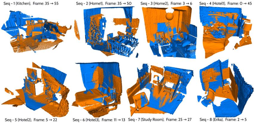
S. A. Ali et al.: Fast Gravitational Approach for Rigid Point Set Registration
centroids (suppose these are originating from prior matches
– Ybc1 . . . Ybcm , where C = {(b c1 , c̃1 ), . . . , (b
cm , c̃m )} is a set of
correspondence indices with entries b cY ∈ {1, . . . , M } and
c̃X ∈ {1, . . . , N }) is defined as:
P
λibc 8(kYi − Ybc k) if C 6= ∅
B(Yi ) = bc∈C (18)
1.0, if C = ∅.
RBFs are invariant under Euclidean transformations,
which is suitable for embedding in iterative alignment meth-
ods, especially for adaptive
2 mass computation. In FGA,
we choose 8(s) = exp − σs 2 . The computational complex-
ity of evaluating B, which is to determine λibc by collocation
on all M template points from a sparse set of m anchor points,
is O(Mm2 ) (O(Nm2 ) for X). Note that m is usually small.
The interpolated masses with three centroids are highlighted
in Fig. 4-A-(middle).
2) NORMALIZED INTRINSIC VOLUME MEASURE
The first step is to discretize each D-dimensional input point
cloud into %D equispaced lattices L, where % = 16 in our
method. These lattices contain scattered density information
across the domains X and Y of X and Y, respectively. Each
of the non-empty lattice cells in L that cover only the domain
of input point cloud, (e.g., Y of Y) has equal intrinsic
FIGURE 3. (A): BH tree structure with hierarchical cell grouping and
pruning depends on the node opening criteria θ . (B): BH force volume (or total quermassintegrals V [85]), of either Lx × Ly
approximation Fθ [30] under different values of the node opening in 2D or Lx × Ly × Lz in 3D. These 2
parameter θ for a template point set (in green color). The red dots R lattices are L u Y, and
represent the CoM of the cells with sizes proportional to the number of
their combined intrinsic volume is LuY V (L). Recall that the
points inside the nodes. lattices are either sparsely or densely packed by the convex
bodies B(Yi ) centered at the locations of all Yi . Each of these
bodies has constant intrinsic volume V (B(Yi )) = π( b−a 2d% )
2
over multiple frames [81] can also increase the corre- in 2D or V (B(Yi )) = 3 π( 2d% ) in 3D. The NIV value of
4 b−a 3
spondence reliability during the registration. In contrast, Yi , contained inside the lattice cell LYi , is expressed as the
point-based [19] or geometric features [82] extracted from the inverse of the ratio Rbetween the V (∪i∈LYi B(Yi )) and V (LYi ),
input can help to boost the correspondence search. Whereas and normalized by LuY V (L):
it is seemingly useful for [36] to add feature descriptors
!−1
from [19] for robust registration, Golyanik et al. [51] suggest 1 V (∪i∈LYi B(Yi ))
to define a separate GMM probability density function for N(Yi ) = R . (19)
LuY V (L) V (LYi )
a prior set of landmarks. Reference [83] can extract the
sensor’s viewpoint signatures as well as the underlying geom- The area (for 2D) or volume (for 3D) fraction of lat-
etry descriptors from considerably noisy point clouds, which tices covered either by the circles (convex bodies for 2D)
helps to estimate 6 DOF camera pose in [84]. or spheres (convex bodies for 3D) centered around the
We define the boundary conditions in two ways, and show enclosed points as the structure descriptors3 is termed as
how they guide Y for robust alignment, especially in the case normalized intrinsic volume (NIV) measure. Fig. 4-A-(right)
of partially overlapping and noisy data. We use (1) a set shows color-coded NIV values of LiDAR scan points and the
of known one-to-one correspondences as landmarks and (2) NIV measure details are depicted in Fig. 4-B.
point cloud feature-based weights as point masses. We finally
derive a (3) Smooth-Particle Mass (SPM) map using RBFs 2 ‘‘u’’ denotes set intersection on a discretized domain
and NIV measures for assigning weights to each point as its 3 The motivation of this descriptor comes from the Monte-Carlo Impor-
input masses. tance Sampling technique — suppose m samples are drawn using some
function f from an alternative population (presented by probability density
function q(x)) of the actual population (presented by R probability density
1) RBF MASS INTERPOLATION function p(x)), then the expected value of
h the samples
i f (x)p(x)dx can also
R f (x)p(x) f (x)p(x)
An RBF [31] is a radially symmetric function around a central be expressed as q(x) q(x)dx = E q(x) . The probability fraction
point. For any given input vector Yi , an RBF interpola- w(x) = p(x) are the importance weights, such that the normalized importance
P q(x)
tion using a radial kernel 8 : RD × RD → R with m radial is mi=1 w(x i ) = 1.
VOLUME 9, 2021 79067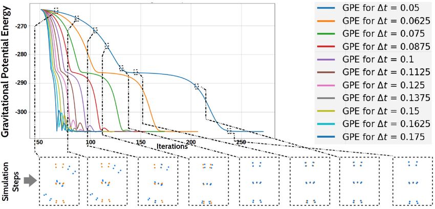
S. A. Ali et al.: Fast Gravitational Approach for Rigid Point Set Registration

                                                                                 Algorithm 2 Fast Gravitational Approach
                                                                                  Input: reference XN ×D , template YM ×D , landmarks
                                                                                          C = (bc, c̃)
                                                                                  Output: optimal rigid transformation T∗ registering Y
                                                                                            to X
                                                                                  Parameters: , η, G, %, 1t, θ, σ
                                                                                  Initialization: T = [R = I3×3 |t = 03×1 ]
                                                                                  normalize X, Y in the range [a, b]
                                                                                  compute B(Y), B(X) using Eq. (18)
                                                                                  compute N(Y), N(X) using Eq. (19)
                                                                                  τ θ ← build BH tree on X with SPM S(X) using Alg. 1
FIGURE 4. (A): The SPM function S maps different point-wise feature
                                                                                  while kTt+1t − Tt−1t k2F ≤ 10−4 do
values to the masses. Shown are the FPFH [19] and the estimated                       compute Ft using Eqs. (5), (7), and (12)
RBF [31] values using landmarks, as well as NIV measures for the mass                 F for k = 1 to M do
initialization of bunny and KITTI [86] data. (B): A lattice representation of
a 2D point set and the visualization of the intrinsic volume defined as the               FθYk ← BHForce(root(τ θ ), Yk , f = 0)
fraction of the cell area occupied by all Yi -centric balls B(Yi ) inside it.
                                                                                       compute Vt+1t and Dt+1t using Eqs.   (8)–(11)
                                                                                       compute transformation Tt+1t ← Rt+1t |tt+1t
3) SPM: SMOOTH-PARTICLE MASS FUNCTION
                                                                                       F solve for Rt+1t using [11], [38], [41], and Eq. (15)
                                                                                       F solve for tt+1t using Eq. (16)
FGA assigns point-wise features as their masses. If landmarks
                                                                                       F update Yt+1t ← (Rt+1t )Yt + tt+1t
are available, we choose strong weights on them and radially
                                                                                       F R ← (Rt+1t )R; t ← tt+1t + (Rt+1t )t;
interpolated weights on the rest of the points using the RBF
map [31] B(Y, C) : RM ×D → RM ×1 . If no landmarks are                            T∗ = [R|t]
available, we use NIV measure N(Y) : RM ×D → RM ×1 .                              Function BHForce(node(τ θ ), Yk , f ):
                                                                                            node(τ θ ).l                  θ
                                                                                                   θ ).CoMk < θ and node(τ ) not empty
The values of the feature maps are spatially smooth. In some                         if kY −node(τ
                                                                                          k
scenarios when point densities are non-uniform and prior                             then
matches are available, then the Hadamard product, symbol-                                f ← f + Force between Yk and node(τ θ ) using
ized by ◦, of RBF and NIV                                                                Eq. (5)
                                                                                     else
                              S=N◦B                                    (20)
                                                                                         for i = 1 to 2D do
assigns balanced weights on X and Y. Alternatively, we can                                   f ← f + BHForce(node(τ θ ).childi , Yk , f )
also map other point-based or geometry-based feature values                            return f ;
(e.g., FPFH [19] or CGF [82]) as SPMs to the masses, which
updates the matrices MX = S(X ) and MY = S(Y ). FGA is
summarized in Alg. 2.
                                                                                forces on every template point. In this process, no synchro-
H. IMPLEMENTATION DETAILS                                                       nization barriers are required to summarize forces.
Many-body simulation is computationally expensive and
demands scalability of its underlying interaction algorithm.                    V. EXPERIMENTAL RESULTS
Fitting BH algorithm on parallel hardware [79] is not                           We evaluate FGA on a wide range of real and synthetic
straightforward as irregular tree data structure cannot be                      datasets with multiple types of data disturbances (e.g., noise
mapped easily to modern uniform memory access architec-                         and partial overlaps). The experiments cover indoor as well
ture. We modify the C++/CUDA implementation blueprint                           as outdoor scenarios, and we compare FGA to several state-
for BH-tree-based n-body simulation [87] method to use in                       of-the-art approaches from different method classes.
our FGA. We describe only the force approximation kernel                           Experimental Datasets: We use the Synthetic bunny
of [87] which is changed for the CUDA/C++ version of                            dataset4 from the Stanford scans repository in the runtime
FGA. The rest of the kernels — bounding box kernel, tree                        experiments (the version with ∼35k points, see Sec. V-B),
building kernel, node-summarizing kernel, node-sorting ker-                     as well as for emulating effects of added synthetic noises and
nel and rigid alignment kernel — for FGA are straightforward                    other data disturbances (the version with ∼1.8k points, see
operations (i.e., either matrix multiplications or sorting).                    Sec. V-E). ModelNet40 [88] is another synthetic dataset com-
   Following Lemma 1, we allocate global memory blocks                          prised of multiple instances of 40 different object categories
for necessary book-keeping tasks on 2D N◦ children indices,                     (e.g., plant, vase, toilet, and table). It has ∼9.8k training
N◦ binary flags for empty or non-empty nodes, N◦ starting                       samples and ∼2.4k testing samples to be used by deep
positions and N◦ ending positions of nodes of integer type
variables. In total, M threads are launched to compute the                        4 www.graphics.stanford.edu/data/3Dscanrep/

79068                                                                                                                                             VOLUME 9, 2021
S. A. Ali et al.: Fast Gravitational Approach for Rigid Point Set Registration

learning methods. In Sec. V-A, we first compare deep                                a few comparisons on ModelNet40 [88] dataset where deep-
learning methods and our FGA (a non-neural method) for                              learning-based methods such as PointNetLK [17] and Deep
the generalizability across different input data. Stanford                          Closest Point (DCP) [15] are exposed to generalization gaps,
lounge5 [89] and Freiburg6 [34] datasets contain partial                            i.e., they perform poorly when tested on data with point
scans of indoor scenes generated using RGB-D sensors. They                          disturbances not observed in the training data. We show that
are widely-used in evaluations of methods for simultaneous                          such neural methods make strong assumptions about the types
localization and mapping (SLAM) where the ratio between                             of data they can deal with. Hence, they are not in the focus of
the area of intersection and the whole inputs — further                             this article.
referred to as the ratio of overlaps — for the consecutive                             FGA runs on a heterogeneous platform with CPU
frames is moderate (i.e., > 50%, and often > 80%). We apply                         (C++ code) and GPU (in CUDA/C++ code). All exper-
FGA on these two datasets and another more challenging                              iments are performed on a system with the Intel Xeon
dataset of similar type with indoor scenes 3DMatch [10]                             E3-1200 CPU with 16GB RAM and NVIDIA 1080 Ti graph-
(in Sec. V-D), where the ratio of overlaps between the                              ics card. We scale our input data in the range [−5, 5] to
source and target frames is lower (i.e., < 50%, and often                           build the BH tree on the reference X up to a fixed depth
< 30%) which makes it highly challenging for point set align-                       of d = 20, as mentioned in Sec. IV-F. In all experiments,
ment methods. Next, we use several driving sequences from                           RBF kernel width (σ ), NIV lattice resolution (%), gravita-
the KITTI7 [86] and Ford8 [90] datasets which contain                               tional constant (G), gravitational force softening length (),
non-uniformly sampled point clouds generated using Velo-                            time integration step (1t), force damping constant (η) and
dyne LiDAR sensors.                                                                 BH-cell opening criteria (θ) are set as — σ = 0.03, % = 16,
   Evaluation Criteria: Bunny dataset provides ground-truth                         G = 66.7,  = 0.2, 1t = 0.1, η = 0.2 and θ = 0.6.
correspondences, and the lounge dataset [89] provides                               Finally, we show through experiments with different datasets
ground-truth transformations (Rgt , tgt ). We calculate the                         that these settings are optimal. FGA converges in 80 − 100
root-mean-squared error (RMSE) on the distances between                             iterations.
registered source and target point clouds with known corre-
spondences and angular deviation ϕ for the lounge dataset,                          A. FGA AGAINST DEEP LEARNING METHODS
which can be measured as the chordal distance between the                           This section provides a detailed analysis of the registra-
estimated (R∗ ) and ground-truth (RTgt ) rotations or as an Euler                   tion results using state-of-the-art deep learning methods —
angular deviation [91]:                                                             PointNetLK [17] and DCP [15] on the ModelNet40 [88]
            180◦  −1                                                            dataset. Both methods are trained from scratch (to account
       ϕ=          cos      0.5(trace(RTgt R∗ ) − 1) .       (21)                   for noisy samples) for 250 epochs with a learning rate of
              π
                                                                                    10−3 using ADAM optimizer [92]. While a batch size 32
   For KITTI [86] and 3DMatch [10] datasets, we measure the                         is used for PointNetLK with ten internal iterations, DCP is
angular deviation ϕ and Euclidean distance 1t between the                           trained with batch size 10 (as recommended in [15], [17]).
translation components t∗ (estimated) and tgt (ground truth).                       Scalability of processing large point clouds is a common
We also report the total transformation error:                                      problem for both these methods (also, both networks have
                         1T = ϕ + ktgt − t∗ k                                (22)   to use a fixed number of multi-layer perceptrons (MLPs) to
                                  | {z }                                            match the embedding dimensions). Hence, we subsample all
                                              1t
                                                                                    CAD shapes to 2048 points. To enhance the accuracy of both
in the experiments for parameter selection in Sec. V-G, where                       the networks in handling data with disturbing effects, we
the angular error ϕ is a small residual part of 1T.                                 perform data augmentation. We randomly select 950 CAD
   Baseline Methods and Parameter Settings: FGA is a                                objects from the training set of ∼9.8k samples and merge
general-purpose registration method which does not require                          them into a single extended training set after applying four
training data and which performs equally well on volumetric                         different types of data disturbances — (i) adding 10% Gaus-
point clouds and also on data with well-defined surface geom-                       sian noise with zero mean and the standard deviation of 0.02,
etry. We hence focus on comparisons to methods making the                           (ii) adding 10% (out of 2048 points) uniformly distributed
same assumptions and report alignment results of CPD [21],                          noise in the range [−0.5, 0.5], (iii) adding perturbations to the
GMMReg [20], FilterReg [16], FGR [13], RANSAC [19],                                 actual point positions with maximum displacement tolerance
point-to-point ICP [6] and GA [11] as well as our FGA. All                          of 0.01, and finally (iv) removing 20% of the points in a
these methods, like our FGA, do not require information on                          chunk at random. The choice of applying the above four
prior correspondences and any special geometric knowledge                           disturbances on any given sample is random (in all of the
about the inputs. However, if available, prior correspondences                      above cases, the total amount of points remains 2048 for
can be used by FGA as boundary conditions. We also include                          each CAD sample). For comparing the errors, we prepare
  5 www.qianyi.info/scenedata.html                                                  five different validation sets — originating from the same
  6 https://vision.in.tum.de/data/datasets/rgbd-dataset                             test set — with increasing levels of the aforementioned data
  7 www.cvlibs.net/datasets/kitti/raw_data.php                                      disturbance types — i.e., by adding 1%, 5%, 10%, 20%, and
  8 http://robots.engin.umich.edu/SoftwareData/Ford                                 40% noisy points or cropping the same amount of points.

VOLUME 9, 2021                                                                                                                                 79069
S. A. Ali et al.: Fast Gravitational Approach for Rigid Point Set Registration
In spite of training with the additional 950 samples, both
DCP and PointNetLK show a common generalizability issue,
see the transformation error plots in Fig. 5. The evaluation
shows that error metrics of PointNetLK becomes signifi-
cantly higher when the noise level increases just from 1% to
5% (for Gaussian noise, the rotational error increases from
4.37◦ to 79.3◦ , and the translational error increases from
0.0252 to 6.05, whereas for uniform noise, the rotational
error increases from 4.29◦ to 78.42◦ , and the translational
error increases from 0.0249 to 3.43). While DCP approach
is more robust than PointNetLK, the noise intolerance issue
is still pertinent for it. Our FGA is far more robust compared
to both neural approaches, i.e., its transformation estimation
errors, especially rotational errors, are consistently smaller by
more than 15 times compared to PointNetLK and ≈1.2 times
compared to DCP. Only the rotational error of FGA is close —
but still lower at several increasing noise levels — compared
to the DCP’s error for cropped inputs.
We conclude that there exist generalization gaps and
robustness issues in these neural approaches when tackling
noisy data which is often encountered in practical applica-
tions. Hence, further in the experimental section, we keep our
focus on unsupervised and general-purpose RPSR methods
which do not require training data and can generalize across
various alignment scenarios.
FIGURE 5. The accuracy of our FGA and two deep learning methods
PointNetLK [17] and DCP [15] trained on ModelNet40 [88] dataset, with
B. FGA RUNTIME AND ACCURACY ANALYSIS additional 10% of the samples included in the training set after applying
four different types of data disturbances. Our FGA is compared on five
To evaluate the runtime versus accuracy of FGA, we take different validation sets with increasing levels of data disturbances. The
a clean bunny with ≈35k points and subsample it with error plots show that FGA outperforms the other two methods and
ten increasing subsampling factors. Ten (X, Y) pairs are highlight the robustness issues of the learning-based approaches.
obtained applying random rigid transformations on each Y.
Fig. 6 illustrates the computational throughput on a CPU of noise and data discontinuities, choosing a higher range of
in frames per second and the accuracy as RMSE of FGA θ ∈ [0.7, 1] is not suitable to trade speed for accuracy gain.
(for θ = 0.5, 0.6, 0.7) against other methods, i.e., CPD [21], Note that a spiking effect is observed on the runtime curve for
GMMReg [20], FilterReg [16], FGR [13], RANSAC [19], ≈35k points in Fig. 7. The reason is that for larger point sets,
point-to-point ICP [6] and GA [11]. FGA ranks top in terms the number of opened nodes does not continuously change
of its computational throughput and accuracy for large point (increase or decrease) for a continuous change on the θ value.
set sizes. Only FilterReg [16] and FGR [13] rival our method Moreover, due to the same reason, the alignment process can
on a small subset of cases, see Fig. 6-(B) for a bivariate require a different number of iterations to converge.
correlation plot for RMSE and the registration speed. Thanks
to the full data parallelization of FGA, its GPU version runs C. PARTIALLY OVERLAPPING DEPTH DATA
∼100 times faster than its CPU version and also outperforms In RGB-D based SLAM, globally-optimal rigid alignment
in speed all other tested CPU versions. Note the GPU version provides camera trajectories by mapping partial scenes. For
of FGA corresponds entirely to the CPU version, and the our quantitative evaluation, we choose the first 400 frames
negligible discrepancy in the RMSE is due to differences in of depth data from Stanford lounge [89] dataset. We next
floating-point calculations between CPU and GPU and the perform registration on every fifth frame (see Fig. 8) after
possible different number of iterations. down-sampling those to ≈5000 points each and report the
The multi-pole acceptance criteria θ reduces the number final Euler angular deviation ϕ (no prior matches are used
of BH tree traversals with its increasing value from 0 to 1. in this experiment). Three different success rates of FGA are
The effect of increasing θ to reduce the computational time measured as the percentages of total experimental outcomes
of FGA is reflected in Fig. 7. The reason for the speed-up is when ϕ is below three different cut-off levels –4◦ , 3◦ ,, and 2◦ ,
that the information about the nodes (positions and masses) respectively. Moreover, we report the average, mini-
at higher depths are being summarized by the nodes of the mum and maximum angular errors denoted by ϕavg. , ϕmin
same type at a lower depth. In the range θ ∈ (0, 0.6], the loss and ϕmax , respectively, see Table 1. On CPU, FGA
of accuracy in the gravitational force approximation is neg- takes around 1.2 seconds on average until convergence
ligible. Note that for some datasets with a high percentage (in 30 − 60 iterations) and performs as the second most
79070 VOLUME 9, 2021S. A. Ali et al.: Fast Gravitational Approach for Rigid Point Set Registration
TABLE 1. The success rate of compared methods for three upper bounds
(4◦ , 3◦ , 2◦ ) on angular deviation from ground truth after registration.
GMMReg [20] and FilterReg [16] all perform poorly on par-
tial data and particularly on 3DMatch. Furthermore, subsam-
pling of 3DMatch scans with a voxel size of 3 cm results in
point clouds with ∼15k points which is still computationally
expensive for these methods. The evaluation includes 506,
156, 207, 226, 104, 54, 292 and 77 challenging pairs from the
3DMatch sequences. Fig. 9 depicts sample registration results
of FGA on pairs of scans from all eight sequences. Fig. 10
shows the total number of successful registrations using FGA
and its runtime compared to other benchmark methods on this
FIGURE 6. (A:) Throughput of different methods in frames per second and dataset. We have also chosen a strict upper bound on rota-
(B:) Bivariate correlation plot for the alignment accuracy and speed, for
ten data sizes and random initial misalignments. The bottom right area of
tional error (S. A. Ali et al.: Fast Gravitational Approach for Rigid Point Set Registration
FIGURE 9. Sample pairwise registration results of our method on all eight different test scenes in 3DMatch [10] dataset. The input point set pairs exhibit
minimal overlaps and irregular cropped areas. The template Y is colored blue and the reference is colored orange. Results of FGA named by the
source-to-target frames (i → j ) are best viewed in color.
FIGURE 11. FGA applied on template and reference point clouds
(frames 1 and 10 from Freiburg [34] dataset). Top row: input images with
the prior correspondenes and the initialization on the right. Bottom row:
Our SPM (S) function radially distributes weights around four different
prior landmarks (highlighted by blue lines), and the alignment on the
right.
to it (a) 40% (of M ) random Gaussian, (b) 40% (of M )
random uniformly distributed noise. We next (c) transform
FIGURE 10. Our FGA is tested on eight evaluation sets of 3DMatch [10] the samples randomly with angular deviations ϕx , ϕy , and ϕz
dataset. We define a strict measurement (i.e., when the angular error is
less than 5◦ and translational error is less than 20 centimeters) to count where all are ∈ U(0, 3π 4 ). We prepare 100 such independent
successful registrations. Top plot: The success rate of FGA is compared test samples for each of the three cases and report success
against the previously well-performing methods — FGR [13], RANSAC [19]
and two other baseline methods — GA [11] and ICP [6]. Bottom plot: FGA
rate when RMSE value is 60% of input data), the NIV (N) measure
To evaluate the robustness of FGA against different disturbing can be constant (e.g., N(X) and N(Y) = 1). FGA is more effi-
effects, we take a clean bunny with 1889 points and add cient and accurate in registering substantially misaligned data
79072 VOLUME 9, 2021You can also read