Measurements on the transport of suspended particulate matter in the Vlie Inlet
←
→
Page content transcription
If your browser does not render page correctly, please read the page content below
Net her lands Jour nal of Geos cie nces —– Ge ologie en Mijnbou w | 9 3 – 3 | 95 -10 5 | 2014                                          doi: 10.1017/ nj g.2014.7

                      Measurements on the transport of suspended particulate
                      matter in the Vlie Inlet

                      T. Gerkema 1,* , J.J. Nauw 1 & C.M. van der Hout 1

           1   NIOZ Royal Netherlands Institute for Sea Research, Texel
           *   Corresponding author. Email: gerk@nioz.nl

           Manuscript received: 11 July 2013, accepted: 13 March 2014

                      Abstract

           Results are presented from campaigns carried out in March and May 2012 across the main channel of the Vlie Inlet in the western Dutch Wadden Sea.
           On both occasions current velocities and concentrations of suspended particulate matter (SPM) were measured at six stations over one tidal cycle.
           Concentrations are found to be high only during late ebb and early flood, implying a brief but intense export and import of SPM, respectively. Trans-
           port of water and SPM occurs predominantly over the southwestern part of the channel. The tidal prism in the channel varies in the range of 5–7 3
           108 m3. Gross amounts of SPM transported during ebb and flood are 6–8 3 106 kg during the first campaign, but only half that amount during the
           second, possibly due to a different wind direction. The limitations encountered when calculating net effects over a tidal cycle are discussed, such as
           the fundamental indeterminacy in the duration of the tidal period itself.

           Keywords: tidal inlet, sediment transport, tidal prism, optical backscatter

                      Introduction                                                                     Geological evidence suggests that barrier-island systems
                                                                                                   like the Wadden Sea are typically sedimentation areas (van
           The western Dutch Wadden Sea is connected to the North Sea by                           Straaten, 1964). An important question is whether the Wadden
           several tidal inlets (Fig. 1). Of these, the Marsdiep and Vlie are                      Sea is presently a net importer of sediment from the North Sea.
           predominant in terms of tidal prism (mean tidal volumes).                               A recent analysis (for sand and silt together) suggests this to be
           Louters & Gerritsen (1994) give as their values 1054 and 1078                           the case: comparisons between bathymetric surveys from 1935
           million m³, respectively; for the other inlets, the tidal prism                         till 2005 show a net sedimentation (Elias et al., 2012). In part,
           is much smaller.                                                                        this must be a response to the closure of the Zuiderzee in 1932;
              The Vlie is the oldest inlet. During the early Subatlanticum                         the main channels of Marsdiep and Vlie were cut short by the
           (∼3000–1000 BP), it was the only pathway from the North                                 dyke and the remaining parts have since become shallower to-
           Sea to the inner lake (Zagwijn, 1991), the later Zuiderzee and                          wards their landward edges.
           present IJsselmeer. Subsequently, human activities (such as                                 An alternative and more direct way to look into the exchange
           peat excavation and compactification due to drainage) made                              of sediment between the North Sea and the Wadden Sea is by
           the coastal areas more vulnerable for flooding. Around 1200                             doing in situ measurements on the transports through the
           AD the Marsdiep was formed, opening up the western part of                              inlets. For suspended particulate matter (SPM) this requires si-
           the Dutch Wadden Sea. This part is thus, by geological stand-                           multaneous measurements of current velocities and concentra-
           ards, very young. By this time, the rate of Holocene sea-level                          tion covering the whole vertical. Such measurements, however,
           rise had already much declined and the rapid accumulation of                            are typically too short to warrant conclusions regarding the net
           sediment in the coastal zone, characteristic of the Atlanticum                          balance of the Wadden Sea; they merely provide a snapshot of
           and Subboreal (∼8000–3000 BP), was long over (Beets & van                               what actually is an episodic process in the long run. Van
           der Spek, 2000). This explains why this part of the Wadden                              Straaten (1975) outlined the role of two opposing effects that
           Sea has a much lower coverage of intertidal flats.                                      play on different time scales: on the one hand, weak net imports

           © Netherlands Journal of Geosciences Foundation 2014                                                                                                             95
Downloaded from https://www.cambridge.org/core. IP address: 46.4.80.155, on 27 Dec 2020 at 06:19:27, subject to the Cambridge Core terms of use, available at https://www.cambridge.org/core/terms
. https://doi.org/10.1017/njg.2014.7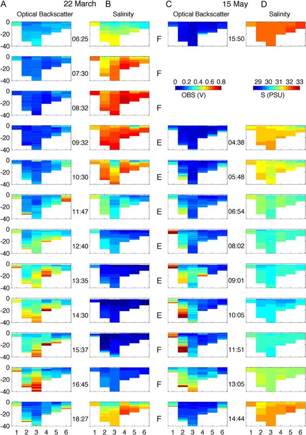
Netherla nds Jour n al of Geos cience s —– Geo logie en M ijnbo uw                     9 3 – 3 | 2 014

           Fig. 1. (a) The location of the Western Dutch Wadden Sea is indicated by the red rectangle. Its bathymetry is shown in (b), with depth in metres. The tran-
           sect of the six stations in the Vlie is indicated as a blue line. All points higher than 1 m above NAP are considered to be ‘land’ in this figure and are rendered
           white. The inset shows the profile of the main channel of the Vlie (depth vs longitude, based on our ADCP measurements) along with the six stations.

           by tidal currents during periods of predominantly calm conditions                                 Study area
           and, on the other hand, large but brief exports during heavy storms,
           when silt is washed off the intertidal flats. It is the net effect of                   The Vlie inlet, measured from island to island, has a width of 7.6 km.
           these two that ultimately determines the long-term evolution.                           This poses a hurdle for doing in situ measurements: if the entire
           To capture this net effect, in situ measurements would need to be                       stretch were covered, the sampling within the tidal cycle would be
           sustained over periods of years. At present, this is done only in                       insufficient. For this reason we restricted our measurements to
           the Texel Inlet, Marsdiep (Nauw et al., 2014).                                          the main channel, at a location where it is at its narrowest. The
               This leaves us with a gap of knowledge regarding the other po-                      six stations are shown in Fig. 1 and their coordinates are given in
           tentially important inlet, the Vlie. A current research project (ZKO                    Table 1; they cover a distance of 1.4 km. Over this stretch, every sta-
           PACE) aims to examine the transport of SPM in the Wadden Sea using                      tion can be sampled some 12 times during the 13-hour measure-
           numerical models (GETM/GOTM and Delft3D). In support of this ef-                        ments. The obvious limitation of this approach is that we will miss
           fort, we carried out two 13-hour measurements across the main                           an unknown but certainly significant part of the transports through
           channel of the Vlie Inlet, on 22 March and 15 May 2012, using                           the inlet, namely those over adjacent flats and through some smaller
           the NIOZ R/V Navicula. This involved current velocities measured                        channels that are also part of the Vlie Inlet.
           with an acoustic doppler current profiler (ADCP), vertical profiles                        The 13-hour measurements were carried out along the same
           of optical backscatter (OBS), and water samples and filtering to de-                    transect on 22 March and 15 May 2012. On 22 March, 12 cross-
           termine SPM concentrations. The results are reported in this paper.                     ings were made from stations 1 to 6 (and return crossings with-
               The main objective of these measurements lies in estimating the                     out casts). On 15 May, 10 crossings were made. Near the end of
           gross import and export during a tidal cycle, rather than in their dif-
           ference, the net effect. From the preceding discussion it will already                  Table 1. Position and waterdepth of the stations.
           be clear that net amounts of transport of SPM over one tidal cycle,
           even if we were able to reliably infer them from the measurements,                      Station      Longitude         Latitude            Depth (m)        Depth (m)
           would not be indicative of the long-term evolution of the Vlie basin.                                                                      22 March         15 May
           Moreover, the fundamental question arises whether such net quan-                        1            5° 09.2499        53° 18.7259         6.4 6 0.2        7.1 6 0.8
           tities can be properly determined in the first place; upon closer in-                   2            5° 09.4049        53° 18.8589         32.6 6 0.5       32.1 6 0.5
           spection, ‘the’ tidal period (the duration over which the net effect is                 3            5° 09.5589        53° 18.9899         39.6 6 0.5       39.9 6 0.8
           to be calculated) is an ambiguous concept, as we will discuss below.
                                                                                                   4            5° 09.7129        53° 19.1219         20.8 6 0.9       20.4 6 0.9
               The purpose of these 13-hour measurements is thus twofold:
                                                                                                   5            5° 09.8739        53° 19.2569         17.0 6 0.2       16.9 6 0.2
           first, to get a synoptic view of the temporal and spatial variabil-
                                                                                                   6            5° 09.9709        53° 19.3419         11.0 6 0.3       10.8 6 0.6
           ity of the transport of SPM within a tidal cycle and, second, to
           obtain estimates of the amounts of SPM involved in the gross                            The waterdepth (with respect to NAP) is based on ADCP data together
                                                                                                   with data from the tidal gauge at Vlieland Haven to correct for sea-level
           import and export during that cycle. This provides crucial data                         variations (tides and wind surges).
           against which future models can be tested.                                              The errors indicate standard deviations.

                96
Downloaded from https://www.cambridge.org/core. IP address: 46.4.80.155, on 27 Dec 2020 at 06:19:27, subject to the Cambridge Core terms of use, available at https://www.cambridge.org/core/terms
. https://doi.org/10.1017/njg.2014.7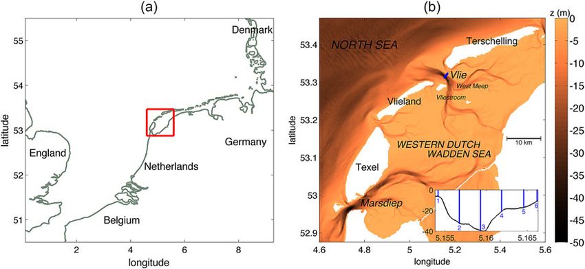
Net her lands Jour nal of Geos ciences —– Ge ologie en M ijnbouw                       93 – 3 | 2014

           Table 2. Tidal characteristics.                                                                   Instruments and data handling

                                                  22 March                    15 May                    From OBS to SPM
           High water (predicted)                 7:56 (+72)                  15:25 (+80)
           High water (measured)                  7:50 (+56)                  15:40 (+101)         CTD/OBS vertical profiles (with Seabird/Seapoint sensors; CTD,
           Slack (flood to ebb)                   9:00                        -
                                                                                                   conductivity temperature depth) were taken at all stations dur-
                                                                                                   ing each crossing from stations 1 to 6 (but not during return
           Low water (predicted)                  14:00 (-126)                9:06 (-100)
                                                                                                   crossings). Water samples (using a Niskin bottle) were taken
           Low water (measured)                   14:20 (-141)                9:20 (-82)
                                                                                                   at stations 1, 3 and 5, both at the surface and at the bottom.
           Slack (ebb to flood)                   15:04                       10:20
                                                                                                   Subsamples were filtered (oven dried and pre-weighed filters),
           Predictions and measured high/low waters are for Vlieland Haven                         and subsequently dried and weighed to obtain the concentra-
           (data from RWS). The water level is mentioned in brackets, in centimetres
           with respect to NAP. Predicted values are based purely on tidal compo-                  tion of SPM. The Niskin bottle, however, was on a different
           nents and do not include wind surges. Measured sea levels are given only                winch than the CTD/OBS frame and therefore at a different po-
           once every 10 min and so have that margin of uncertainty for the times
                                                                                                   sition in the water, so these SPM values cannot be directly used
           of measured high and low waters. Times of slack are based on the
           measurements presented here, calculated for the bulk water transport.                   to translate the OBS profiles into SPM profiles. To connect them,
           The turn from flood to ebb on 15 May fell after the campaign was halted.                we also measured the OBS value for each water sample, using
           All times are in UTC.
                                                                                                   another OBS sensor in the laboratory on board the ship. A
           the second campaign, a combination of strong winds and flood                            calibration between the two OBS sensors then allowed us,
           currents made it impossible to stay close to stations during the                        finally, to translate OBS profiles from the CTD/OBS frame into
           casts; at that point the campaign had to be halted and the last                         OBS values of the sensor in the laboratory, and hence into
           intended crossing was dropped.                                                          SPM concentrations. The procedure is described in more detail
               The conditions were different with regard to both wind and tides.                   by Merckelbach & Ridderinkhof (2006).
           On 22 March, the wind was more or less perpendicular to the channel,                        The main uncertainty in this procedure lies in the relation
           ENE 4–5 Bft. It was two days before spring tides (new moon on 22                        between SPM concentrations and OBS values (taken from the
           March, 14:37 UTC). On 15 May, the wind was stronger and directed                        same sample in the laboratory), as illustrated in Fig. 2. The data
           straight into the inlet: NW 5 Bft, increasing to NNW 7 Bft in the after-                show considerable scatter and are heteroskedastic, i.e. the dispersal
           noon. Neap tides fell on this day (last quarter on 12 May, 21:47 UTC).                  of points is uneven: the spreading becomes larger for larger values.
               The tidal characteristics are summarised in Table 2. We see                         In such cases, with errors not being random, the Theil–Sen method
           that slacks come shortly after high or low waters (within about                         is more appropriate than the commonly used least-squares method
           an hour or less), so already at this location the tides are closer                      (e.g. Sprent 1993), so we adopted the former. The Theil–Sen method
           to a standing than to a propagating wave. In line with the pre-                         is also less sensitive to outliers.
           vailing wind directions, water levels were lower than predicted                             For 15 May, the steepness of the linear fit is only 70% of that
           on 22 March and higher than predicted on 15 May (see values in                          for 22 March. This is possibly related to the fact that current
           brackets, Table 2).                                                                     velocities were higher on 22 March (e.g. blue lines in Fig. 7),

           Fig. 2. OBS values against SPM concentrations. Black circles refer to
           surface samples; blue crosses to bottom samples. In each panel, the
           linear fit (red line) is based on surface and bottom data together.
           Also indicated are the fits for the subsets of surface (black dashed
           line) and bottom (blue dashed line) samples, taken separately.

                                                                                                                                                                            97
Downloaded from https://www.cambridge.org/core. IP address: 46.4.80.155, on 27 Dec 2020 at 06:19:27, subject to the Cambridge Core terms of use, available at https://www.cambridge.org/core/terms
. https://doi.org/10.1017/njg.2014.7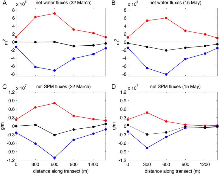
Netherla nds Jour n al of Geos cience s —– Geo logie en M ijnbo uw                     9 3 – 3 | 2 014

           so that relatively more coarser-grained material was brought                            recorded with the CTD frame is never the same during revisits
           into suspension, to which OBS sensors respond less strongly.                            of what is, nominally, the same station. The other reason, of
           In other words, a higher concentration would be needed on                               course, is that from one visit to the next the surface height
           22 March than on 15 May to get the same OBS output. This ex-                            changes with the tide and variable wind surges. These two vari-
           planation gains further plausibility if we look at fits for bottom                      able factors pose the problem of how to connect, for the same
           or surface samples taken separately (in Fig. 2: blue and black                          station, the vertical data points from different crossings.
           dashed lines, respectively). For bottom samples the lines are                              We deal with these obstacles in the following way. It turns
           steeper than for surface samples, implying that a higher con-                           out that the ADCP was close to the true location of a station
           centration is needed for the former to get the same OBS value.                          during at least some of the time of a cast. Thus, we select the
           This fits in with the fact that coarser-grained sediments                               N profiles that are closest to the station. Of these N profiles,
           (e.g. fine sand) are generally more prevalent near the bottom                           we take the median for each vertical bin. We also take the
           than near the surface. In addition, the OBS response is known                           median of the N values for the water depth measured by the
           to be sensitive to other properties, such as particle shape, near                       ADCP (correcting for the fact that the ADCP hangs 1 m below
           infrared reflectivity of the material (’color’), flocculation, phy-                     the surface). From this median water depth we then subtract
           toplankton blooms and more (Downing, 2006). One would need                              the elevation (with respect to NAP) as measured at Vlieland
           additional measurements to determine the importance of these                            Haven, being the nearest tide-gauge station; we thus correct
           factors in the specific setting.                                                        for the effect of tides and wind surges. After these corrections,
              Several sensitivity tests can be done, for example using                             only a slight variation remains in different casts for the same
           separately the subsets of bottom and surface samples in                                 station. This must be due to the (small) variation in location
           constructing calibration lines, as indicated in Fig. 2. The gap                         between different casts, and the imprecision of the ADCP meas-
           between the lines then suggests a relative margin of uncer-                             urements themselves. Finally, we take, for each station, the
           tainty in the order of 15–20%.                                                          median over all casts. We refer to this as the ‘reference depth’,
                                                                                                   the estimated water depth with respect to NAP.
                 Supplementing missing or noisy ADCP data                                             This method appears to work well. Specifically, for 22 March,
                                                                                                   we choose N = 10. The distance of the selected profiles to their
           A downward looking 1.2 kHz RDI Workhorse ADCP was mounted                               corresponding station is, on average, only 12 m, so the profiles
           at a pole on the R/V Navicula. It sampled over 88 bins of 0.5 m                         can reasonably be considered to be taken ‘at’ the station. The
           and a profile was logged every 3 s. Because of side-lobe inter-                         reference depth is shown in Table 1, together with the standard
           ference, the ADCP data become noisy and unreliable in about                             deviation, which is a measure of the variation between differ-
           the lowest 10% of the water column; for the deepest station                             ent casts at the same station. Notice that in most cases this
           3, as much as the lowest 35% shows noisiness. These parts were                          deviation is actually smaller than the bin size, so no better
           replaced by the simple empirical profile proposed by van Veen                           accuracy could be expected.
           (1937), u =a h1/5.2, which he showed works well for the Vlie Inlet                         For 15 May, the ADCP data contained more noise, so we
           (here u is the velocity component, a is a constant chosen to fit                        included more profiles: N = 20. The mean distance to corre-
           the higher part of the profile and h is the height above the bottom).                   sponding stations was now 15 m. The reference shows a larger
              The ADCP did not function during the first three casts on                            standard deviation, but, given these error bars, the median
           22 March, so the profiles of stations 1 to 3 are missing from                           values are consistent with those of 22 March.
           the first crossing. These were constructed heuristically by                                Finally, it is convenient to put all the measured variables of
           taking a linear combination of the profiles from the second                             the vertical profiles into a fixed grid, to be used throughout.
           and, close to a tidal period later, the last two crossings. As a test,                  Integration over time then becomes particularly straightfor-
           we applied the same construction to stations 4 to 6: the result-                        ward, since each specific gridpoint can be treated separately.
           ing profiles bore a fair resemblance to the measured ones from                          Thus, we introduce a vertical axis on which, for each station,
           these stations. In any case, concentrations of SPM were very low                        the bottom is fixed at a level z =-hb, where hb is the highest
           during this first crossing (as discussed below), so any error in                        water level (i.e. the reference depth of that station plus high
           these profiles is inconsequential for the overall SPM fluxes.                           water). So, by definition, the water surface reaches z = 0 during
                                                                                                   high water, but lies lower at all other times. In the latter case,
                 Reference levels for the vertical                                                 the gridpoints in between are assigned the value ‘infinite’ and
                                                                                                   are rendered white in the figures presented here (e.g. in Fig. 4).
           Although the same stations 1 to 6 were visited during succes-                           For time integrations concerning these gridpoints, there is no
           sive crossings, in practice this is only true in a loose sense,                         contribution from such moments.
           for the vessel cannot stay exactly at that position during the                             We choose a vertical grid distance of 0.25 m (as in the CTD
           casts; moreover the CTD frame itself drifts away during its low-                        data), which is half that of the ADCP bin size. For each cast,
           ering and hoisting. This is one reason why the water depth                              the ADCP profile is filled into the new grid from the bottom

                98
Downloaded from https://www.cambridge.org/core. IP address: 46.4.80.155, on 27 Dec 2020 at 06:19:27, subject to the Cambridge Core terms of use, available at https://www.cambridge.org/core/terms
. https://doi.org/10.1017/njg.2014.7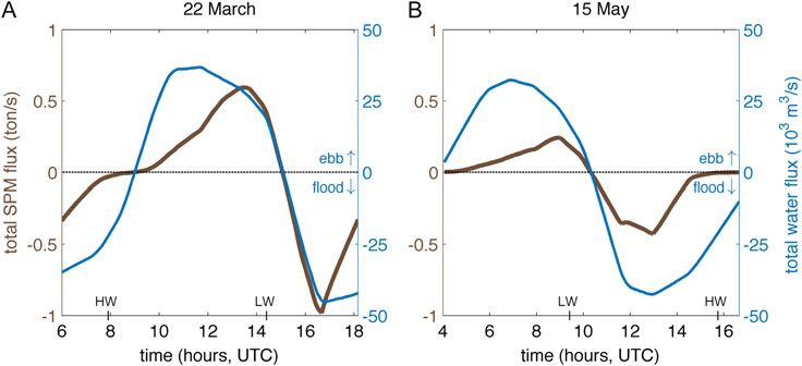
Net her lands Jour nal of Geos ciences —– Ge ologie en M ijnbouw 93 – 3 | 2014
upwards and interpolated to the finer grid size. At the top, data values are included as correctly as possible, leaving extrapola-
were missing in the upper 2 m, and this was filled up by tions to near-surface values, which is the lesser evil so far as
constant extrapolation, i.e. assigning the upper value to the sediment transport is concerned.
missing points above it, up to the level of the free surface
during that cast. The CTD/OBS data are similarly filled in from Results
below. Due to drifts of the ship and CTD frame, the frame may
have landed at a deeper or shallower position than the station Spatial and temporal variations
in question. In the former case, there are more data than
needed for the grid and redundant data points are left out; in We start by showing the results from the CTD/OBS casts in
the latter case, there are not sufficient data and the missing Fig. 3, which give a first impression of the spatial and temporal
near-surface values are filled in with constant extrapolation. characteristics of the transports in the Vlie Inlet. We recall
Thus, we work our way from the bottom upwards (instead of that the measurements of 15 May do not cover a full tidal cycle
from the surface downwards), ensuring that the near-bottom (missing the later f lood stage) and have two transects less than
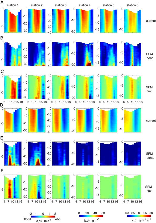
Fig. 3. Results from the CTD/OBS casts
along the transect. For 22 March, time
progresses from upper to lower panels,
but for 15 May the panels have been
slightly re-ordered to make the tidal
phases correspond more closely to those
of 22 March for easier comparison; thus,
the last transect is plotted first. In each
panel, the vertical indicates depth in
metres; on the horizontal, the station
number is given. The indicated time (in
UTC) is the average during the crossing
from stations 1 to 6. The phase of the
tidal current is marked by E (ebb) and
F (flood).Colour bars apply to both
dates.
99
Downloaded from https://www.cambridge.org/core. IP address: 46.4.80.155, on 27 Dec 2020 at 06:19:27, subject to the Cambridge Core terms of use, available at https://www.cambridge.org/core/terms
. https://doi.org/10.1017/njg.2014.7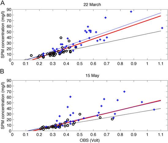
Netherla nds Jour n al of Geos cience s —– Geo logie en M ijnbo uw                     9 3 – 3 | 2 014

           on 22 March. We show OBS and salinity. The time of day is                               from the eastern f lats and watershed into the West Meep, thus
           indicated in a cross-transect average sense; typically, the                             giving more supply to the eastern part of the main channel.
           crossing from station 1 to 6 took about three quarters of an
           hour. The phase of the tide at that stage is indicated by E or F                             Local flux of SPM
           (ebb or f lood).
               Both for 22 March (panel columns a and b) and 15 May (panel                         The northern and eastern current velocities from the ADCP were
           columns c and d), a remarkable correspondence in the overall                            rotated over an angle of 54.8° to transform the signal into
           phases is seen between OBS and salinity: when the former is                             cross- and along-transect components. The latter is typically
           high, the latter is low, and vice versa.                                                five to ten times weaker than the cross-transect current; it
               The lowest values of salinity are seen during ebb, as expected                      would become still weaker if we reduced the angle slightly
           since the fresh water from the landward side of the Vlie basin                          (by about 7°), indicating that our transect is not perfectly
           (mainly originating from the sluice at Kornwerderzand) is then                          normal to the principal flow. This is, however, immaterial to
           exported. However, salinity stays low during the early stage of                         the cross-transect transports that we calculate hereafter. For
           f lood, which means that the relatively fresh water that was                            the cross-transect flow, we adopt the convention that negative
           brought to the outer delta during ebb is being imported again                           values correspond to a flow into the Wadden Sea (flood)
           at the beginning of f lood. Conversely, relatively saline water                         and positive values to a flow into the North Sea (ebb). Profiles
           is exported at the beginning of ebb.                                                    coinciding with CTD casts were obtained as explained in
               During half of the tidal cycle – during late flood and early                        the previous section. For each station the profiles were linearly
           ebb – OBS values are low throughout. Only in the later stages                           interpolated (and where necessary extrapolated) to a 5-min
           of ebb do they rise, starting from the shallow sides of the                             timeline covering a full tidal period. (The duration of the tidal
           channel. Then, the deepest part of the channel (stations 2                              period is, in fact, intrinsically ambiguous; we examine this
           and 3) gains importance and finally becomes dominant at the                             problem in the section Discussion.) This timeline is chosen to
           beginning of flood, when high values are confined to those                              be the same for all stations, to facilitate comparisons between
           two stations. The broad picture is thus one of an export of                             them. OBS values were treated similarly and translated into SPM
           SPM during late ebb, predominantly over the shallower sides                             concentrations via the calibration lines of Fig. 2.
           adjacent to the intertidal flats, and a brief import through                               The evolution of the cross-transect velocity and SPM concen-
           the central channel during early flood.                                                 tration is shown in Fig. 4 for both campaigns. Each station has
               These measurements show how OBS varies locally (i.e. at this                        been given the same vertical extent in the panels, but notice
           particular transect), but the origin of the signal, like that of                        that their water depths (and hence the vertical scales) vary
           fresh water, lies presumably farther into the basin. The main                           greatly. This is also the reason why the white areas in the upper
           channels in the Wadden Sea are known to be predominantly                                layer, marking the void due to low water, are more clearly visible
           sandy (van Straaten, 1964), so the (re)suspended sediments                              in the outer panels, where the effect is relatively large because
           that pass the transect will generally have travelled some                               of the shallowness of the stations.
           distance before they arrive at the transect. This idea gains plau-                         In Fig. 4, rows a and d, we see that the current amplitude
           sibility from the fact that the OBS signal becomes strong only                          decreases substantially from stations 1 to 6, while the phases
           during the second half of the ebb phase. We can estimate the                            hardly differ between the stations. In Fig. 4, rows b and
           corresponding distance. With typical maximum current speeds                             e, SPM concentrations are plotted. The scale is limited at
           of about 1.5 m s–1, the tidal excursion is obtained by dividing                         60 g/m³; higher values are only sporadically reached. Here we
           this maximum by the (semidiurnal lunar) tidal frequency,                                see phase differences between the stations: the shallow
           giving about 10 km; this is the distance traversed by water                             stations generally precede the deeper ones with regard to peak
           parcels during the first half of ebb. The sediment that we see                          values in SPM. In all cases the concentrations decrease strongly
           arriving at that point, therefore, must come from within a circle                       towards the surface. By contrast, the flux (Fig. 4c,f), obtained
           of about 10 km. The circle includes the intertidal flats adjacent                       by multiplying current velocity and concentration, is on the
           to the Vliestroom and West Meep channels.                                               whole rather more homogeneous in the vertical. This means
               Meanwhile, clear differences are seen between the two cam-                          that the upward decrease in concentration is largely offset by
           paigns. On 22 March, the distribution of OBS values is more or                          an upward increase in current velocity. (In cases when only
           less symmetric across the channel, but on 15 May the pattern is                         surface data are available, it would thus make more sense to
           strongly skewed towards its southwestern side (i.e. stations                            assume that the fluxes stay constant over the vertical than
           1 and 2), suggesting that the supply comes now mainly from                              to assume this for SPM concentrations.) For the fluxes, the western
           the western branch, Vliestroom, and adjacent intertidal flats.                          half of the channel is dominant, especially so on 15 May. This skew-
           It is not evident whether this difference is due to wind direction                      ness to the western side can be ascribed to two factors: first, tidal
           or wind strength, although it is natural to expect that with the                        currents are stronger on the western side (Fig. 4a,d) and, second,
           ENE winds on 22 March more sediment would be transported                                phases of currents and SPM concentrations are more in unison

              100
Downloaded from https://www.cambridge.org/core. IP address: 46.4.80.155, on 27 Dec 2020 at 06:19:27, subject to the Cambridge Core terms of use, available at https://www.cambridge.org/core/terms
. https://doi.org/10.1017/njg.2014.7
Net her lands Jour nal of Geos ciences —– Ge ologie en M ijnbouw 93 – 3 | 2014
Fig. 4. Results for 22 March (rows a–c)
and for 15 May (rows d–f): the cross-
transect tidal current (rows a,d), the
SPM concentration (rows b,e) and their
product (rows c,f), based on linear inter-
polation of the data to 5-min intervals
and extrapolation to a full tidal period.
The six columns represent stations 1 to
6. In each panel, time is on the horizontal
axis (hours UTC) and the depth with respect
to HW (in metres) is on the vertical axis.
at western stations. For example, on 22 March (Fig. 4a,b), fluxes (see Fig. 4c,f), but due to its shallowness the contribu-
maximum concentrations occur around slack at station 4, tion to the total transport is relatively modest (Fig. 5c,d).
whereas at station 1 maximum concentrations occur before In all cases, stations 2 and 3 are predominant in the vertically
and after slack, resulting in higher f luxes. integrated transports. Regarding the transport of water, a dom-
inance of flood is found on both occasions (see black lines in
Tidal prism and transport of SPM Fig. 5a,b), but on 15 May it is more pronounced, which is not
surprising in view of the strong NNW wind. In all panels there
Starting from Fig. 4, rows c and f, we can now, for each station, is a pronounced asymmetry, a skewness to the left (i.e. south-
vertically integrate the instantaneous fluxes and calculate west), most clearly so for the SPM f luxes on 15 May (Fig. 5d).
the overall transport during ebb and flood. Thus, the real Finally, we can horizontally integrate the results shown
contribution from the different stations is cast into a more in Fig. 5; this yields the values gathered in Table 3. The water
proper perspective. For example, station 1 has the highest local volumes differ between the two days of measurements.
101
Downloaded from https://www.cambridge.org/core. IP address: 46.4.80.155, on 27 Dec 2020 at 06:19:27, subject to the Cambridge Core terms of use, available at https://www.cambridge.org/core/terms
. https://doi.org/10.1017/njg.2014.7Netherla nds Jour n al of Geos cience s —– Geo logie en M ijnbo uw 9 3 – 3 | 2 014
Fig. 5. Fluxes for water and SPM at sta-
tions 1 to 6 (from left to right), inte-
grated over the vertical and in time for
ebb and flood, separately. The timespans
of ebb (red) and flood (blue) are inte-
grated separately. The net result of the
two is shown as the black line.
As expected, the NNW wind on 15 May reduced the export of wa- at Vlieland Haven, which showed a rise in sea level over each of
ter and increased the import. the 13-hour periods (the rise can be largely ascribed to the di-
Our values for the tidal prism are significantly smaller than urnal inequality, along with wind effects on 15 May). There is
earlier estimates for the entire inlet. These estimates, it should a caveat, however, for the rise in level is not necessarily due
be noted, are themselves subject to a large margin of variability: to an inflow through the Vlie alone; other sources may have
reported values range from 880 million m³ (Postma, 1982) to contributed, namely exchanges with the adjacent basins and
1078 million m³ (Louters & Gerritsen, 1994). Similar margins discharges from the sluices. The latter is negligible for the dates
occur in an analysis by Hut (2004). These variations are to we are concerned with here. It is in any case natural to assume
be expected: not only does the tide vary in intensity (e.g. that the Vlie Inlet must be the chief contributor; by lack of
spring-neap cycles), but the tidal prism (in spite of its name) further data, we shall ignore the possible exchanges with the
is also strongly inf luenced by non-tidal effects, notably the adjacent basins.
wind, which causes it to be highly variable. In a numerical On 15 May, the tidal gauge at Vlieland Haven shows that
modelling study, covering two years with realistic forcing, the water level rose from +50 cm at the start of the campaign
Duran-Matute et al. (2014) found that the standard deviation to +86 cm one tidal period later. For an estimated area of the
of tidal prisms is typically about 20% of their long-term average Vlie basin of 668 km² (for mean high water, see Elias et al.,
(for the Vlie: 934 million m³). All reported values fall easily 2012), this implies an overall import of –240 3 106 m³. This
within that margin. corresponds well with the net import we find for 15 May
Our measurements cover only the main channel. Some idea (–177 3 106 m³, following from Table 3), which, after extrapo-
of how much we miss (in comparison with the entire inlet) lation to the entire inlet, amounts to –221 3 106 m³. A margin
can be deduced from the different transects covered by Visser
et al. (1986). They give values for a transect similar to ours, al- Table 3. The total exports during ebb and imports during flood of the water
though it extended possibly somewhat farther to the east. That volumes and mass of SPM.
transect alone accounts for about 80% of the total tidal prism
(Visser et al., 1986), so we may assume a similar percentage Export Import
in our case. Extrapolated to the entire inlet, our average value 22 March 6
Water (10 m³) 576 –633
for the tidal prism then approaches the lower bound of the SPM (106 kg) 6.6 –7.8
range in the numerical study by Duran-Matute et al. (2014). 15 May 6
Water (10 m³) 497 –674
For the water volumes, a net import is seen on both days.
SPM (106 kg) 2.4 –4.1
This is qualitatively in agreement with data from the tidal gauge
102
Downloaded from https://www.cambridge.org/core. IP address: 46.4.80.155, on 27 Dec 2020 at 06:19:27, subject to the Cambridge Core terms of use, available at https://www.cambridge.org/core/terms
. https://doi.org/10.1017/njg.2014.7Net her lands Jour nal of Geos ciences —– Ge ologie en M ijnbouw 93 – 3 | 2014
of error as small as 2% in the gross volumes would already be are incommensurable. For exactly the same reason it has been
sufficient to accommodate the mismatch with the value derived impossible to construct a calendar that truly ref lects these
from the tidal gauge. astronomical periods.
A similar exercise can be done for 22 March; here the discrep- By way of example, we use the tidal predictions for Vlieland
ancy is slightly larger: a net import of –71 3 106 m³ from Table 3 Haven. By restricting ourselves to the predicted signal, we will
(after extrapolation to the entire inlet) compared to an be dealing only with tidal components and ignoring wind
imported volume of –107 3 106 m³ according to the rise in surges. In Fig. 6 we compare the time between successive low
sea level at the tidal gauge. For the gross volumes, an uncer- waters (red dots) with the time between successive high waters
tainty of 4% is now sufficient to resolve the discrepancy. (blue dots) for the months of March to May 2012. Both are
These comparisons show that the net tidal prisms are even plotted as the shift with respect to the reference period of
quantitatively in good agreement with independent data from the semidiurnal lunar tidal period (M2, 12 h 25 min). The lunar
the tidal gauge. For the transport of SPM, however, the gross phases of full and new moon are also indicated. Four things are
amounts are subject to a much larger range of uncertainty apparent from this figure. First, the overall pattern follows the
due to the conversion from OBS values to SPM concentrations spring-neap cycle: times between successive low (or high)
(Fig. 2). Several sensitivity tests can be done, for example using waters are generally shorter than the M2 period during spring
only the bottom samples in constructing the calibration line. On tides (i.e. about two days after full or new moon), while they
that basis, we estimate that in the gross amounts, uncertainties exceed the M2 period during neap tides, sometimes by as much
may be as large as 20–30%. As a result, the net effect of import as three quarters of an hour. (Thus, with regard to tidal prism,
and export together must be regarded as unreliable, as it falls lower current amplitudes during neap tides are partially offset
entirely within the margin of error. Qualitatively, however, by the longer duration of its period.) Second, diurnal inequal-
a net import of sediment (as suggested by the values in Table ities are clearly visible as up- and downward jumps in subse-
3) does make sense in our case; after all, along with the net im- quent points of the same colour. Thus, not only the water
port of water, one may expect an import of sediment. level itself is affected by the diurnal inequality, but also
the period. Third, even though the overall pattern is stamped
by the spring-neap cycle, irregularities abound in the
Discussion: indeterminacy in the duration
details– a manifestation of the aperiodic character of the tide,
of the tidal cycle
a direct result of the incommensurability of the underlying
astronomical periods. Fourth – the most important point
In the preceding sections we have made reference to the tidal
for the present discussion – the time between successive
cycle. In practice, its duration is taken as the time between suc-
low waters is sometimes nearly identical to the time between
cessive low waters, or between successive high waters, or
successive high waters of that same day, but it can also be
between alternate slacks. However, these options produce
very different (by as much as half an hour). In the latter case,
different results. This problem seems to have received little
it becomes ambiguous how ‘the’ tidal period should be
attention in the literature; for this reason, we think it useful
defined.
to include a short intermezzo on it here.
In the case at hand, we have for 22 March as the time
Naturally, the wind is a perturbing factor in this, but even if
between successive low waters 12 h 12 min, and between high
we restrict ourselves to purely tidal components, the ambiguity
waters 12 h 10 min. For 15 May the departure was larger: the
in the definition of ‘the’ tidal period persists. This unavoidable
time between successive low waters was 12 h 44 min and be-
problem derives directly from the fact that the underlying astro-
tween high waters was 12 h 29 min. For both days we took
nomical periods (associated with the Earth’s rotation on its
the average for the duration of the time integration. With
axis, the yearly motion around the sun, the lunar period etc.)
Fig. 6. The time between successive low waters (in red) and between successive high waters (in blue), shown as departures from the M2 tidal period
(horizontal grey line). These durations are based on tidal predictions for Vlieland Haven for the months of March to May. The campaigns described in this
paper took place on yearday 82 (22 March) and 136 (15 May), as indicated by arrows. The lunar phases of full moon (open circle) and new moon (black
circle) are also indicated.
103
Downloaded from https://www.cambridge.org/core. IP address: 46.4.80.155, on 27 Dec 2020 at 06:19:27, subject to the Cambridge Core terms of use, available at https://www.cambridge.org/core/terms
. https://doi.org/10.1017/njg.2014.7Netherla nds Jour n al of Geos cience s —– Geo logie en M ijnbo uw 9 3 – 3 | 2 014
Fig. 7. Temporal evolution of the trans-
ports of SPM (brown) and water (blue),
spatially integrated over the vertical
plane of the transect.
regard to the transport of SPM, the problem can be somewhat plays indeed only a minor role in the net export of fresh water;
mitigated by starting and ending the measurements at instead, the key players are the Marsdiep and the watershed
moments when concentrations are low; the integrated result south of Terschelling (Duran-Matute et al., 2014). Future
is then less sensitive to the choice of the endpoint in time. modelling studies may shed light on whether the Vlie plays
As luck would have it, this is the case in our campaigns (cf. a similarly minor role in the net transport of SPM. The Marsdiep,
Fig. 3a,c). on the other hand, is known to have an import of SPM from the
North Sea (Nauw et al., 2014). The Marsdiep is also the first
tidal inlet encountered by the northward ‘river’ of silt along
Conclusion
the Dutch coast (de Kok, 2004) and is thus (literally) in a
more favourable position than the Vlie when it comes to sources
In this study, the transport of water and SPM through the
of SPM.
Vlie Inlet was examined using data from two measurement
Besides common features, notable differences between
campaigns covering a tidal cycle, on 22 March and 15 May
the campaigns also stand out in Fig. 7. The tidal currents were
2012. The conditions differed with respect to tides and wind,
overall slightly stronger on 22 March than on 15 May
but common features can be identified. First, with regard to
(Fig. 7, blue lines), although for the flood phases this differ-
the spatial distribution, the transport of water and SPM is con-
ence is masked by the effect of the strong NNW wind on
centrated in the southwestern part of the deep channel (Fig. 5).
15 May. The difference in amounts of transport of SPM is much
This conforms to the asymmetric cross-channel bathymetry
more pronounced (Fig. 7, brown lines): they are much smaller
itself (Fig. 1). Second, a distinct pattern is found in the tempo-
on 15 May. More insight into the origin of this difference is
ral evolution: SPM concentrations and transports are low during
provided by the spatial view in Fig. 4: on 15 May less than half
late flood and early ebb; the transport occurs predominantly
the channel (only the western side) contributes to the transport
before and after the slack from ebb to flood. This is further
of SPM, as opposed to 22 March, when the entire channel is in-
illustrated in Fig. 7, which condenses previous results by
volved. A tentative explanation is that the eastern side may
showing the spatially integrated transports of water and SPM
have received a supply of SPM from the eastern intertidal flats
as a function of time. The overall picture is that SPM starts to
and adjacent watershed (via the channel West Meep, Fig. 1)
arrive at the inlet during the later stages of ebb, initially via
due to ENE winds on 22 March, but not when the wind is NNW,
the shallow sides adjacent to intertidal flats, is exported
as on 15 May. Numerical model simulations should be a useful
towards the outer delta, but returns at the beginning of flood
tool to examine such possible dependences on wind direction
via the deeper parts of the channel, after which the concentra-
in a systematic manner.
tions dwindle again. This suggests that the transports during
the tidal cycle amount by and large to a reshuffling of SPM
within the tidal basin, rather than to a genuine exchange be- Acknowledgements
tween the North Sea and the Wadden Sea – an idea put forward
already by Dronkers (1984). We thank the crew of the R/V Navicula for their assistance, Sven
In this respect there is a similarity with fresh water, which Ober for technical support and all who helped carrying out the
leaves during late ebb and (at least partially) returns during measurements: Simona Aracri, Jurre de Vries, Meinard Tiessen
early flood (Fig. 2). Although no conclusions can be drawn from and Matias Duran Matute. Carola van der Hout was supported by
these measurements on the long-term net balance, an analysis Ecoshape/BwN project NTW3.1. Janine Nauw was supported by
using a realistic numerical model demonstrates that the Vlie ZKO project 83908230.
104
Downloaded from https://www.cambridge.org/core. IP address: 46.4.80.155, on 27 Dec 2020 at 06:19:27, subject to the Cambridge Core terms of use, available at https://www.cambridge.org/core/terms
. https://doi.org/10.1017/njg.2014.7Net her lands Jour nal of Geos ciences —– Ge ologie en M ijnbouw 93 – 3 | 2014
References
Beets, D.J. & van der Spek, A.J.F., 2000. The Holocene evolution of the barrier
and the back-barrier basins of Belgium and the Netherlands as a function
of late Weichselian morphology, relative sea level rise and sediment supply.
Netherlands Journal of Geosciences 79: 3-16.
de Kok, J.M., 2004. Slibtransport langs de Nederlandse kust. Bronnen, fluxen
en concentraties. Report RIKZ/OS/2004.148w, Rijkswaterstaat (Den Haag):
25 pp.
Downing, J., 2006. Twenty-five years with OBS sensors: The good, the bad, and the
ugly. Continental Shelf Research 26: 2299-2318.
Dronkers, J., 1984. Import of fine marine sediment in tidal basins. In: Laane,
R.W.P.M. & Wolff, W.J. (eds): The role of organic matter in the Wadden Sea,
Proceedings of the 4th International Wadden Sea Symp. Netherlands Institute
for Sea Research, Publication Series 10-1984 (Texel): 83-105.
Duran-Matute, M., Gerkema, T., de Boer, G.J., Nauw, J.J. & Gräwe, U., 2014.
Residual circulation and fresh-water transport in the Dutch Wadden Sea:
a numerical modeling study. Ocean Science doi:10.5194/osd-11-197-2014,
submitted.
Elias, E.P.L., van der Spek, A.J.F., Wang, Z.B. & de Ronde, J., 2012. Morphody-
namic development and sediment budget of the Dutch Wadden Sea over the
last century. Netherlands Journal of Geosciences 91: 293-310.
Hut, H.J., 2004. Stroommeting buitendelta zeegat tussen Vlieland en Terschelling
27 augustus 2002: project VLIEDEBI. Report DNN-AM-2003-212 (in Dutch).
Rijkswaterstaat (Delfzijl): 19 pp.
Louters, T. & Gerritsen, F., 1994. Het mysterie van de wadden: hoe een getijdesysteem
inspeelt op de zeespiegelstijging (in Dutch). Report RIKZ-94.040. Rijkswaterstaat
(Den Haag): 70 pp.
Merckelbach, L.M. & Ridderinkhof, H., 2006: Estimating suspended sediment
concentration using backscatterance from an acoustic Doppler profiling
current meter at a site with strong tidal currents. Ocean Dynamics 56: 153-168.
Nauw, J.J., Merckelbach, L.M., Ridderinkhof, H. & van Aken, H.M., 2014.
Long-term ferry-based observations of the suspended sediment fluxes
through the Marsdiep inlet using acoustic Doppler current profilers. Journal
of Sea Research 87: 17-29.
Postma, H., 1982. Hydrography of the Wadden Sea: movements and properties of
water and particulate matter. Balkema (Rotterdam): 75 pp.
Sprent, P., 1993. Applied nonparametric statistical methods, 2nd edn. Chapman &
Hall (London): 342 pp.
van Straaten, L.M.J.U., 1964. De bodem der Waddenzee (in Dutch). In:
Abrahamse, J., Buwalda, J.D. & Van Straaten, L.M.J.U. (eds): Het
Waddenboek. Thieme (Zutphen): 75-151.
van Straaten, L.M.J.U., 1975. De sedimenthuishouding in de Waddenzee
(in Dutch). In: Swennen, C., De Wilde, P.A.W.J. & Haeck, J. (eds): Symposium
Waddenonderzoek. Mededeling nr. 1 van de Werkgroep Waddengebied
(Stichting-Veth, Arnhem): 5-20.
van Veen, J., 1937. Waarnemingen omtrent de snelheidsverdeeling in een
verticaal. Rapporten en Mededeelingen van den Rijkswaterstaat, № 29
(in Dutch). Alg. Landsdrukkerij (’s Gravenhage): 45 pp.
Visser, C., de Graaff, N. & de Boer, M., 1986. Het vermogen van het Zeegat van het
Vlie. Report ANW-86.H205 (in Dutch). Rijkswaterstaat (Hoorn): 20 pp.
Zagwijn, W.H., 1991. Nederland in het Holoceen, 2nd edn. Sdu (Den Haag): 46 pp.
105
Downloaded from https://www.cambridge.org/core. IP address: 46.4.80.155, on 27 Dec 2020 at 06:19:27, subject to the Cambridge Core terms of use, available at https://www.cambridge.org/core/terms
. https://doi.org/10.1017/njg.2014.7You can also read