Meta-Reinforcement Learning in Broad and Non-Parametric Environments
←
→
Page content transcription
If your browser does not render page correctly, please read the page content below

Meta-Reinforcement Learning in Broad and
                                                      Non-Parametric Environments

                                                           Zhenshan Bing                                    Lukas Knak
                                                      Department of Informatics                       Department of Informatics
                                                    Technical University of Munich                  Technical University of Munich
                                                          Munich, Germany                                 Munich, Germany
arXiv:2108.03718v1 [cs.LG] 8 Aug 2021

                                                          bing@in.tum.de                                lukas.knak@tum.de

                                                      Fabrice Oliver Robin                                 Kai Huang
                                                    Department of Informatics                  School of Data and Computer Science
                                                  Technical University of Munich                      Sun Yat-sen University
                                                        Munich, Germany                                 Guangzhou, China
                                                       morinf@in.tum.de                          huangk36@mail.sysu.edu.cn

                                                                                     Alois Knoll
                                                                            Technical University of Munich
                                                                                  Munich, Germany
                                                                                 knoll@in.tum.de

                                                                                       Abstract
                                                 Recent state-of-the-art artificial agents lack the ability to adapt rapidly to new tasks,
                                                 as they are trained exclusively for specific objectives and require massive amounts
                                                 of interaction to learn new skills. Meta-reinforcement learning (meta-RL) addresses
                                                 this challenge by leveraging knowledge learned from training tasks to perform
                                                 well in previously unseen tasks. However, current meta-RL approaches limit
                                                 themselves to narrow parametric task distributions, ignoring qualitative differences
                                                 between tasks that occur in the real world. In this paper, we introduce TIGR, a
                                                 Task-Inference-based meta-RL algorithm using Gaussian mixture models (GMM)
                                                 and gated Recurrent units, designed for tasks in non-parametric environments.
                                                 We employ a generative model involving a GMM to capture the multi-modality
                                                 of the tasks. We decouple the policy training from the task-inference learning
                                                 and efficiently train the inference mechanism on the basis of an unsupervised
                                                 reconstruction objective. We provide a benchmark with qualitatively distinct tasks
                                                 based on the half-cheetah environment and demonstrate the superior performance
                                                 of TIGR compared to state-of-the-art meta-RL approaches in terms of sample
                                                 efficiency (3-10 times faster), asymptotic performance, and applicability in non-
                                                 parametric environments with zero-shot adaptation. The videos can be viewed at
                                                 https://videoviewsite.wixsite.com/tigr.

                                        1   Introduction
                                        Humans have the ability to learn new skills by transferring previously acquired knowledge, which
                                        enables them to quickly and easily adapt to new challenges. However, state-of-the-art artificial agents
                                        lack this ability, since they are generally trained on specific tasks from scratch, which renders them
                                        unable to adapt to differing tasks or to reuse existing experiences. For instance, to imbue a robotic
                                        hand with the dexterity to solve a Rubik’s Cube, OpenAI reported a cumulative experience of thirteen

                                        Preprint. Under review.
thousand years [15]. In contrast, adult humans are able to manipulate the cube almost instantaneously,
as they possess prior knowledge regarding generic object manipulation.
As a promising approach, meta-RL reinterprets this open challenge of adapting to new and yet
related tasks as a learning-to-learn problem [5]. Specifically, meta-RL aims to learn new skills
by first learning a prior from a set of similar tasks and then reusing this policy to succeed after
few or zero trials in the new target environment. Recent studies in meta-RL can be divided into
three main categories. Gradient-based meta-RL approaches, such as MAML [6], aim to learn a set
of highly sensitive model parameters, so that the agent can quickly adapt to new tasks with only
few gradient descent steps. Recurrence-based methods aim to learn how to implicitly store task
information in the hidden states during meta-training and utilize the resulting mechanism during
meta-testing [23]. While these two concepts can adapt to new tasks in only a few trials, they adopt
on-policy RL algorithms during meta-training, which require massive amounts of data and lead to
sample inefficiency. To address this issue, PEARL [16], a model-free and off-policy method, achieves
state-of-the-art results and significantly outperforms prior studies in terms of sample efficiency and
asymptotic performance, by representing the task with a single Gaussian distribution through an
encoder which outputs the probabilistic task embeddings.
However, most previous approaches, including PEARL, are severely limited to narrow task distribu-
tions, as they have only been applied to parametric environments [16, 22, 6, 9, 14], in which only
certain parameters of the tasks are varied. This ignores the fact that humans are usually faced with
qualitatively different tasks in their daily lives, which happen to share some common structure. For
example, grasping a bottle and turning a doorknob both require the dexterity of a hand. However, the
non-parametric variability introduced by the two different objects makes it much more difficult to
solve the tasks when compared to the sole use of parametric variations, such as turning a doorknob to
different angles. In spite of these limitations, there is currently no study that explicitly focuses on
challenging non-parametric environment variability while providing the benefits of model-free and
off-policy algorithms, such as the superior data efficiency and good asymptotic performance.
In this paper, we establish an approach that addresses the challenge of learning how to behave in
non-parametric and broad task distributions. We leverage insights from PEARL [16] and introduce
a Task-Inference-based meta-RL algorithm using Gaussian mixture models and gated Recurrent
units (TIGR), which is sample-efficient, adapts in a zero-shot manner, and achieves good asymptotic
performance in non-parametric tasks. We base our method on four novel concepts. First, we use a
generative model, leveraging a mixture of Gaussians to cluster the information on each qualitatively
different base task. Second, we decouple the task-inference training from the RL algorithm by
reconstructing the tasks’ Markov decision processes (MDPs) in an unsupervised setup. Third, we
propose a zero-shot adaptation mechanism by extracting features from recent transition history
and infer task information at each timestep. Last, we provide a benchmark with non-parametric
tasks based on the commonly used half-cheetah environment. Experiment results demonstrate that
TIGR significantly outperforms state-of-the-art methods with 3-10 times faster sample efficiency,
substantially increased asymptotic performance, and unmatched task-inference capabilities under
zero-shot adaptation in non-parametric environments for the first time. To the best of the authors’
knowledge, TIGR is the first model-free meta-RL algorithm to solve non-parametric environments
with zero-shot adaptation.

2   Background

Meta-reinforcement learning The learning problem of meta-RL is extended to an agent that has
to solve different tasks from a distribution p(T ) [24]. Each task T is defined as an individual MDP
specifying its properties. A meta-RL agent is not given any task information other than the experience
it gathers while interacting with the environment. A standard meta-RL setup consists of two task sets:
a meta-training task set DTtrain used to train the agent, and a meta-test task set DTtest used to evaluate
the agent. Both sets are drawn from the same distribution p(T ), but DTtest may differ from DTtrain .
The objective is to train a policy πθ on DTtrain that maximizes rewards on DTtest , which is defined as
                                                   "             "                ##
                                                                     X
                         θ∗ = arg max ET ∼DTtest Eτ ∼p(τ |πθ )           γ t rt        .              (1)
                                   θ                                 t

                                                    2
Figure 1: Visualization of the non-parametric half-cheetah-eight benchmark. From left to right: run
forward, run backward, reach front goal, reach back goal, front stand, back stand, jump, and front
flip. These eight tasks share similar dynamic models, but are qualitatively distinct. Each task contains
parametric variations, e.g., different goal velocities in the run forward/backward task.

Meta-training and meta-testing Meta-RL consists of two stages: meta-training and meta-testing.
During meta-training, each training epoch consists of a data collection and optimization phase. In
the data collection phase, interaction experiences for each task are collected and stored in the replay
buffer. In the optimization phase, the losses for the policy are computed and the gradient of the
averaged losses is used to update the parameters of the policy. During meta-testing, the policy is
adapted to new tasks with either few trials, meaning that the agent can experience the presented
environment and adapt before the final evaluation, or in zero-shot manner, which means that the agent
must solve the environment at first sight.

Parametric and non-parametric variability in meta-RL Two key properties define the under-
lying structure of task distributions in meta-RL [24]: parametric and non-parametric variability.
Parametric variability describes tasks that qualitatively share the same properties (i.e., their semantic
task descriptions are similar), but the parameterization of the tasks varies. Parametric task distri-
butions tend to be more homogeneous and narrower, which limits the generalization ability of the
trained agent to new tasks. Non-parametric variability, however, describes tasks that are qualitatively
distinct but share a common structure, so a single meta-RL agent can succeed (See Figure 1 for a
visual example of non-parametric tasks). Non-parametric task distributions are considerably more
challenging, since each distinct task may contain parametric variations [24].

Probabilistic embeddings for Actor-Critic RL (PEARL) In task-inference-based meta-RL, the
task information that the agent lacks to enable it to behave optimally given a problem T ∼ p(T )
is modelled explicitly [9]. PEARL [16] learns a probabilistic latent variable z that encodes the
salient task information given by a fixed-length context variable cT1:N containing N recently collected
experiences of a task T , which is fed into the policy πθ (a|s, z) trained via soft actor-critic (SAC)
[8] to solve the presented task. To encode the task information, an inference network qφ (z|cT1:N ) is
learned with the variational lower bound objective
                           h                                                      i
                  ET ∼p(T ) Ez∼qφ (z|cT1:N ) R(T , z) + βDKL qφ (z|cT1:N ) p(z)

                                                                                      ,             (2)

where p(z) is a Gaussian prior used as a bottleneck constraint on the information of z, given
context cT1:N using the KL-divergence DKL . R(T , z) is an objective used to train the encoder via
the Bellmann critics loss. β is a hyperparameter for weighting the KL-divergence. The probabilistic
encoder in PEARL is modeled as a product of independent Gaussian factors over the N transitions
                                                                     2
qφ (z|cT1:N ) ∝ n Ψφ (z|cTn ), where Ψφ (z|cTn ) ∼ N (fφµ (cTn ), fφσ (cTn )) and fφ is represented
                Q

as a neural network with parameters φ that outputs the mean µ and variance σ 2 of the Gaussian
conditioned on the context cTn . In the data collection phase, previous experiences are iteratively
added to the context to predict the new latent task representation used in the policy for the next
action. During testing, PEARL performs a few-shot adaptation by first collecting experiences and
then computing a posterior for the latent representation, which remains unchanged during the entire
roll-out. We highly encourage readers to read about PEARL [16] for its intuitive visualizations and
in-depth explanations, as preliminaries to this work.

3   Related Work

The recent work in the domain of meta-RL can be divided into three groups according to the approach
taken: gradient-based, recurrence-based, and task-inference-based.

                                                   3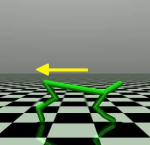
1
                                                        Leuclid         LKL-divergence
                                                                                                 Decoder
                                                                                                                    Ldynamics
                                                      Lclassification                         (State/Reward
                                                                                                                    Lrewards
                                                                                                prediction)
                                               Encoder
       Context c at timestep t             (Task inference)                   Latent
    st−1   at−1         rt−1     st                                          Variable
                                                                                                                2
    st−2   at−2         rt−2    st−1
                                         GRU              GMM                    z
                                                                                             Task-conditioned        Lactor
                  ...                                                                          policy (SAC)          Lcritic
    st−T   at−T         rt−T   st−T +1

Figure 2: Meta-training procedure. The encoder learns a task encoding z from the recent context with
gradients from the decoder and provides z for the task-conditioned policy trained via SAC. Orange
arrows outline the gradient flow.

Gradient-based Gradient-based meta-RL approaches such as MAML [6] and follow-up methods
[1, 3, 14] are based on finding a set of model parameters during meta-training that can rapidly adapt
to achieve large improvements on tasks sampled from a distribution p(T ). During the meta-test phase,
the initial learned parameters are adjusted to succeed in the task with few gradient steps [6].

Recurrence-based The key element in recurrence-based methods, as in [23, 5, 13, 15], is the
implementation of a recurrent model that uses previous interactions to implicitly store information
that the policy can exploit to perform well on a task distribution. By resetting the model at the
beginning of each roll-out and recurrently feeding states, actions, and rewards back to the model,
the agent can track the interaction history over the entire path in its hidden state and learn how to
memorize relevant task information [23]. In meta-training, the model is trained via back-propagation
through time. In meta-testing, the parameters are fixed, but the agent’s internal state adapts to the
new task [23].

Task-inference-based In task-inference-based meta-RL, as in PEARL [16], the information that
the agent lacks to enable it to behave optimally is modelled explicitly [9]. MAESN [7], for example,
learns a task-dependent latent space that is used to introduce structured noise into the observations
to guide the policy’s exploration. The authors of [11] improve on this idea by modelling the task
explicitly using an encoder consisting of a gated recurrent unit (GRU) to extract information from a
history of transitions, which is given to the policy in addition to the observations. In [22], the feature
extraction is improved by leveraging a graph neural network that aggregates task information over
time and outputs a Gaussian distribution over the latent representation. The authors of [18] further
use a combination of a Dirichlet and a Gaussian distribution to model different base tasks with style
factors.

4    Problem Statement

This work aims to solve non-parametric meta-RL tasks, in which an agent is trained to maximize
the expected discounted return across multiple test tasks from a non-parametric task distribution.
Specifically, we aim to achieve the following goals: first, our algorithm should be applicable to non-
parametric and broad task distributions in a meta-RL setting. Second, the developed algorithm must
be able to perform zero-shot adaptation. Finally, the method should provide the sample efficiency and
asymptotic performance of model-free and off-policy algorithms. To the best of our knowledge, there
is no approach that provides the advantages of model-free and off-policy algorithms and is applicable
to non-parametric environments in a zero-shot manner. Currently the only benchmark that satisfies the
environment requirements is Metaworld [24]. Since Metaworld does not offer well-defined rewards
that are normalized across all environments, which can lead to strong bias towards dominant tasks,
we provide our own benchmark half-cheetah-eight to evaluate different meta-RL approaches.

5    Methodology

In this section, we first give an overview of our TIGR algorithm. We then explain the strategy for
making TIGR applicable in non-parametric environments, derive the generative model, and explain
how we implement the encoder and decoder. Finally, we summarize TIGR with its pseudocode.

                                                               4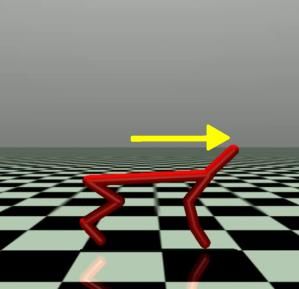
5.1     Overview

In this paper, we leverage the notion of meta-RL as task inference. Similar to PEARL, we also extract
information from the transition history and use an encoder to generate task embeddings, which are
provided to a task-conditioned policy learned via SAC. Unlike PEARL, however, we first redesign
the generative model for the task inference to succeed in non-parametric environments. Second, we
decouple the training of the probabilistic encoder from the training of the policy by introducing a
decoder that reconstructs the underlying MDP of the environment. Third, we modify the training and
testing procedure to encode task information from the recent transition history on a per-time-step
basis, enabling zero-shot adaptation. The structure of our method is shown in Figure 2. Our algorithm
is briefly explained as follows.

         • During meta-training, we first gather interaction experiences from the training tasks and
           store them in the replay buffer. At each interaction, we infer a task representation, such that
           the policy can behave according to the objective in (1). We feed the recent transition history
           into a GRU (Sec. 5.2.1), which merges the extracted information and forward the features to
           the GMM (Sec. 5.2.1) to generate the overall task representation z. The task representation
           is given to the policy with the current observation to predict the corresponding action.
         • Second, we optimize the task-inference and policy networks, in two sequential stages:
             – We first train the GRU-GMM encoder networks for task inference by reconstructing
               the underlying MDP. For this, we use two additional neural networks that predict the
               dynamics and reward for each transition (See orange gradient 1 in Figure 2 and Sec.
               5.2.2). This gives the encoder the information required to generate an informative task
               representation. To improve the performance of the task inference, we employ two
               additional losses, namely, Lclassification and LEuclid (See Sec. 5.2.2). We do not use any
               gradients from SAC (See orange gradient 2 ), which enables us to train the encoder
               independently of the task-conditioned policy.
             – In policy training, we compute the task representation for the sampled transitions online
               using our GRU-GMM encoder. We feed this information to the task-conditioned policy
               and train it via SAC independently of the task-inference mechanism.
         • During meta-testing, our method infers the task representation at each timestep, selects
           actions with the task-conditioned policy and adapts to the task in zero-shot manner.

5.2     Task Inference

The non-parametric environments that we consider describe a broad task distribution, with different
clusters representing the non-parametric base tasks, and the intra-cluster variance describing the
parametric variability for each objective. A standard variational autoencoder (VAE) with a single
Gaussian for the underlying generative model as in PEARL is not intended to represent such clustered
task distributions. We propose a more complex generative model involving a GMM that captures
the multi-modality of the environments and produces reasonable task representations that take into
account both non-parametric and parametric variability.

5.2.1    Generative Model
Given the context c = (st−T , at−T , rt−T , st−T +1 ..., st−1 , at−1 , rt−1 , st ) as the sequence of the
recent transition history in the last T timesteps, we aim to extract features and find a latent representa-
tion z that explains c ∼ p(c|z) in a generative model such that p(c, z) = p(c|z)p(z). We reinterpret
the joint structure of the meta-RL task distribution as a combination of different features in a latent
space that represent the properties of a particular objective. Following this idea, we model z as a
mixture of Gaussians that can express both non-parametric variability with the different Gaussian
modes and parametric variability using the variance of a particular Gaussian k with its statistics
µ(c, k) and σ 2 (c, k). Formalizing this mathematically, we use the following generative model:
                                          X
                                             ρ(c, k) N µ(c, k), σ 2 (c, k)

                               p(z|c) =                                                                (3)
                                          k
                                                                            P
where ρ(c, k) determines the activation for each Gaussian k subject to k ρ(c, k) = 1. Given a
shared structure between tasks, the model thus represents the activated latent features that explain the

                                                     5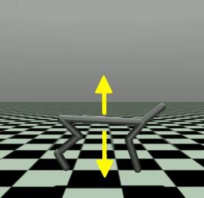
Gaussian Mixture Model
                 Input Features                                                Lclassification
                                                                                 Leuclid
                                        ρ1    ρ2    ...   ρk
                       .                                                           Latent
                       .                                                          Variable
                       .                                          ζ1
                       .                µ1    µ2    ...   µk               +         z
                       .                                          ζ2
                       .
                                                                  ...
                                        σ12   σ22   ...   σk2
                                                                  ζk           LKL-divergence

                                                                Samples

Figure 3: Overview of the GMM network. The statistics for each Gaussian in the mixture, including
mean µ(c, k), variance σ 2 (c, k), and activation ρ(c, k), are computed in parallel. The values are
processed and the task representation z is calculated as the weighted sum denoted by the + as
described in Sec. 5.2.1. Orange arrows outline the gradient flow.

tasks’ properties. In the case of a dominant component with an activation ρ(c, k) → 1, the sum can
be neglected, but for multiple activated components, our method provides more degrees of freedom
than sampling from one Gaussian, as in [17]. We compute µ(c, k), σ 2 (c, k) and ρ(c, k) as described
in the following section.

GMM architecture Using the variational inference approach, we approximate the intractable pos-
terior p(z|c) using a variational posterior qθ (z|c), parameterized by neural networks with parameters
θ. The neural network that implements the GMM is designed as a multilayer perceptron (MLP) that
predicts the statistics for each Gaussian component including the mean µ(c, k), variance σ 2 (c, k) and
activation ρ(c, k) as a function of the input features derived from the context c (See Figure 3). The
standard model is given as a two-layer network and an output layer size of K × (dim(z) × 2 + 1),
where K is the handcrafted number of Gaussian components, dim(z) is the latent dimensionality
required for mean µ(c, k) and variance σ 2 (c, k), and the Gaussian activation value is ρ(c, k). Finally,
we represent the GMM components as multivariate Gaussian distributions with mean µ(c, k) and
covariance Σk = I σ 2 (c, k), where the diagonal of Σk consists of the entries of σ 2 (c, k), while
every other value is 0. This assumes that there are no statistical effects between the tasks. We apply
a softplus operation to enforce that the network output σ 2 (c, k) contains only positive values. We
sample from the multivariateP Gaussian distributions and obtain representatives ζk for each Gaussian
component. We enforce k ρ(c, k) = 1 by computing the softmax over the GMM’s output for the
ρ(c, k) values. Using the computedP activations ρ(c, k) and the representatives, we obtain the final
latent task representation z = k ρ(c, k) · ζk .

Feature extraction In this paper, we consider RL environments that are described as high di-
mensional MDPs. To enable our GMM to produce an informative task representation from the
high dimensional input data, we first employ a feature extraction mechanism to find the relevant
information contained in the context. We employ a GRU to process the sequential input data (See
Appendix Figure 7). We recurrently feed in the transitions of the context c, and thereby combine the
features internally in the GRU’s hidden state. We extract this hidden state after the last transition is
processed and forward it into the GMM. An ablation study of various feature extraction configurations
is presented in Appendix A.6.

5.2.2   Encoder-Decoder Strategy
Our generative model follows the idea of a VAE. The setup employs an encoder, to describe the latent
task information given a history of transitions from an MDP as qθ (z|c); and a decoder to reconstruct
the MDP from the latent task information given by the encoder as pφ (c|z). The encoder is modeled
as a GMM which involves the prior use of a shared feature extraction method, as described in the
previous section. The decoder implements the generating function pφ (c|z), parameterized as neural
networks with parameters φ. Following the variational approach in [10], we derive the evidence lower
bound objective (ELBO) for the encoder and decoder and obtain:
             log pφ (c) ≥ L(θ, φ; c) = Eqθ (z|c) [log pφ (c, z) − log qθ (z|c)]
                                       = Eqθ (z|c) [log pφ (c|z)] − DKL (qθ (z|c)kpφ (z)) .          (4)

                                                           6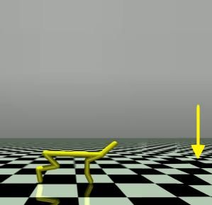
We use the reparameterization trick z̃ = k ρqθ (c, k) µqθ (c, k) +  · σq2θ (c, k) with  ∼ N (0, 1)
                                        P
and apply Monte Carlo sampling to arrive at the objective:

                     L(θ, φ; c) ≈ log pφ (c|z̃) − DKL (qθ (z̃|c)kpφ (z̃)) ,                     (5)

where log pφ (c|z̃) is a reconstruction objective of the input data c. DKL (qθ (z̃|c)kpφ (z̃)) introduces a
regularization conditioned on the prior pφ (z̃). Since the lower bound objective requires maximization,
we denote the optimization objective as minimizing −L(θ, φ; c), which results in a negative log-
likelihood objective for the reconstruction term.

Reconstruction objective The reconstruction objective provides the information necessary for the
encoder and GMM to extract and compress relevant task information from the context. It can take
many forms, as suggested in [16], such as reducing the Bellmann critic’s loss, maximizing the actor’s
returns, and reconstructing states and rewards. We follow the third proposal and extend the negative
log-likelihood objective of reconstructing states and rewards to predicting the environment dynamics
and the reward function for the underlying MDP (See Appendix Figure 8). We split the decoder into
two parts pφdynamics and pφrewards , which predict the next state s0 and reward r given s, a and z, and train
them with the following loss:
                       log pφ (c|z̃) = log pφ (s0 , r|s, a, z̃)
                                      = log pφdynamics (s0 |s, a, z̃) + log pφrewards (r|s, a, z̃).               (6)
We model both parts as regression networks, in which the data is modeled as a normal distribution.
Thus, the loss function is defined as the sum of Ldynamics (φ) and Lrewards (φ) as:
                               1                                           1
        Lprediction (φ) =          ||s0 − pφdynamics (s0 |s, a, z̃)||2 +        ||r − pφrewards (r|s, a, z̃)||2   (7)
                            dim(s)                                       dim(r)
where both components are normalized by the number of their dimensions.

Information bottleneck The regularization introduced by the KL-divergence in (5) serves as an
information bottleneck that helps the GMM compress the input to a compact format. Due to the
potential over-regularization of this term [4], we control its impact on the ELBO as −L(θ, φ; c) ≈
LNLL (θ, φ) + α · LKL-divergence (θ), with a factor α < 1 to allow expressive latent representations.

Clustering losses To improve the task inference performance for non-parametric environments, we
experiment with two additional losses that represent the two following ideas: (1) We enforce that each
component of the GMM is assigned to one base task, similar to the component constraint learning in
[17], using a supervised classification learning approach
                                                            for the activations ρ(c, k) and the true base
                                        exp(ρ(c,k=y))
class y as Lclassification (θ) = − log  P
                                           exp(ρ(c,k)) . (2) We confine the features to separate clusters
                                              k
by maximizing the Euclidean distance between the means µ(c, k) of the K components scaled by
                                                                                                           2
the inverse of the sum of variances σ 2 (c, k) with LEuclid (θ) = k1 =1 k2 =k1 +1 ||µ(c,k
                                                                 PK PK                      1 )−µ(c,k2 )||
                                                                                    σ 2 (c,k1 )+σ 2 (c,k2 ) .
We provide a detailed description of the losses and an evaluation of their impact in Appendix A.5.

Final objective The final objective derived from the reconstruction objective, information bot-
tleneck, and clustering losses is used to jointly train the encoder-decoder setup as described in
Section 5.2.2. We combine the different loss functions to enable the encoder to produce informative
embeddings, which are used in the task-conditioned policy. The resulting overall loss is denoted as:
      L(θ, φ) = LNLL (prediction) (θ, φ) + α · LKL-divergence (θ) + β · LEuclid (θ) + γ · Lclassification (θ)     (8)
where α, β, γ are hyper-parameters that weigh the importance of each term.

5.3     Algorithm Overview

The TIGR algorithm is summarized in pseudo-code (See Algorithm 1). The task-inference mechanism
is implemented from line 3 to line 9. Lines 10 and 12 implement the standard SAC [8]. A list of the
most important hyperparameters of the algorithm and their values is given in Appendix A.2.

                                                            7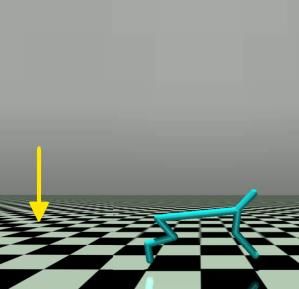
Algorithm 1 TIGR Meta-training
Require: Encoder qθ , decoder pφ , policy πψ , Q-network Qω , task distribution p(T ), replay buffer D
 1: for each epoch do
 2:     Perform roll-out for each task T ∼ p(T ), store in D
 3:     for each task-inference training step do
 4:         Sample context c ∼ D
 5:         Compute z = qθ (c)                                                      . (See Sec. 5.2.1)
 6:         Calculate losses LKL-divergence , LEuclid , Lclassification             . (See Sec. 5.2.2)
 7:         Compute (s0 , r) = pφ (s, a, z)                                         . (See Sec. 5.2.2)
 8:         Calculate loss Lprediction
 9:         Derive gradients for losses with respect to qθ , pφ and perform optimization step
10:     for each policy training step do
11:         Sample RL batch d ∼ D and corresponding context c, infer z = qθ (c)
12:         Perform SAC algorithm for πψ , Qω
    return qθ , πψ

                                           Half-Cheetah Vel-Task                                      Half-Cheetah Dir-Task                                           Ant-Three
                                 0                                                                                                              −50
                                                                                   2000
    Average Return R

                    −100                                                           1500                                                         −100

                                                                                   1000
                    −200                                                                                                                        −150
                                                                                    500
                                                                                                                                                −200
                    −300                                                             0
                                 104              105                 106                       104          105                   106             104        105      106   107         108
                                           Training Transition n                                      Training Transition n                                     Training Transition n
                                                              TIGR          PEARL               PRO-MP                      RL2          MAML            final performance

Figure 4: Meta-testing performance over environment interactions evaluated periodically during the
meta-training phase. As PEARL [16] outperforms ProMP [19], RL2 [5], and MAML [6] in half-
cheetah-vel and half-cheetah-dir, we only compare TIGR with PEARL in these two environments.

                                                   Half-Cheetah-Eight                                                                    Half-Cheetah-Eight
                                 −50
                                                                                                                            40
                                 −75                                                                                                                                              Front flip
                                                                                                                                                                                  Goal in back
              Average Return R

                                                                                                  TIGR
                            −100                                                                                            20
                                                                                                             Latent Dim 2

                                                                                                  PEARL                                                                           Goal in front
                                                                                                  PRO-MP                                                                          Jump
                            −125
                                                                                                  RL2                       0                                                     Back stand
                            −150                                                                  MAML                                                                            Front stand
                                                                                                  final                                                                           Run forward
                                                                                                                        −20
                            −175                                                                                                                                                  Run backward

                            −200                                                                                        −40
                                     104    105         106          107     108          109                                     −40    −20       0           20
                                                   Training Transition n                                                                   Latent Dim 1

                                           (a) Meta-testing performance                                                                   (b) Latent encoding
Figure 5: (a) Meta-testing performance over environment interactions evaluated periodically during
the meta-training phase. We show the mean performance from three independent runs. (b) Final
encoding of the eight tasks visualized using T-SNE [20] in two dimensions.

6                Experiments

We evaluate the performance of our method on the non-parametric half-cheetah-eight benchmark that
we provide and verify its wide applicability on a series of other environments. The half-cheetah-eight
environments are shown in Figure 1 and their detailed descriptions are introduced in Appendix A.1.
The evaluation metric is the average reward during the meta testing phase. We first compare the
sample efficiency and asymptotic performance against state-of-the-art meta-RL algorithms, including
PEARL. Second, we visualize the latent space encoding of the GMM. Third, we evaluate the task-
inference capabilities of our algorithm in the zero-shot setup. Finally, we provide videos displaying
the distinct learned behaviors in the supplementary material, along with our code.

                                                                                                            8
Run forward Goal in front Front stand Jump
10.0 1.5 3.0
4
2.2
3 7.5 1.1 1.5
Distance
Velocity
Velocity
2
Angle
5.0 0.7 0.7
1
0.0
0 2.5 0.3
0.0 0.0
Target Velocity Target Distance Target Angle Target Velocity
0 25 50 75 100 0 50 100 150 200 0 50 100 150 200 0.0 12.5 25.0 37.5 50.0
Time Step t Time Step t Time Step t Time Step t
Figure 6: Task-inference response during one episode for the half-cheetah-eight benchmark after
2000 training epochs. Each task is evaluated under different parametric variations. The target is
marked as the dashed line. The task is inferred correctly when the solid line approaches the target.
Asymptotic performance and sample efficiency We first demonstrate the performance of PEARL
and our method in standard parametric environments, namely half-cheetah-vel and half-cheetah-dir
tasks [16], to verify both approaches. It should be noted that PEARL achieves reported performances
in few-shot manner while our method is tested at first sight in zero-shot fashion. Figure 4 shows that
both methods achieve similar performance and can solve the tasks. However, TIGR significantly
outperforms PEARL in terms of sample efficiency across both tasks, even in zero-shot manner.
We then progress to a slightly broader task distribution and evaluate the performance of PEARL,
other state-of-the-art algorithms, and our method, on a modification of the ant environment. We use
three different tasks, namely goal tasks, velocity tasks and a jumping task. The goal and velocity
tasks are each split into left, right, up, and down and include different parametrizations. We take
the original code and parameters provided from PEARL [16]. For a fair comparison, we adjust the
dimensionality of the latent variable to be the same. For the other meta-RL algorithms, we use the
code provided by the authors of Pro-MP [19].1 Figure 4 on the right shows the performances of these
five methods. We see that although PEARL and RL2 can solve the different tasks, our method greatly
outperforms the others in sample efficiency and has a slight advantage in asymptotic performance.
Finally, we evaluate the approaches on the half-cheetah-eight benchmark. The average reward during
meta-testing is shown in Figure 5a. We can see that TIGR outperforms prior methods in terms of
sample efficiency and demonstrates superior asymptotic performance. Looking at the behaviours
showcased in the video provided with the supplementary material, we find that with a final average
return of −150, the PEARL agent is not able to distinguish the tasks. We observe a goal-directed
behavior of the agent for the goal tasks but no generalization of the forward/backward movement
to velocity tasks. It learns how to stand in the front but fails in stand back, jump and front flip. For
TIGR, we can see that every base task except the front flip is learnt correctly. It should be noted that
for the customized flip task, we expect the agent to flip at different angular velocities, which is much
harder than the standard flip task, in which the rotation speed is simply maximized.
Latent space encoding We evaluate the latent task representation by sampling transition histories
from the replay buffer that belong to individual roll-outs. We extract features from the context
using the GRU encoder and obtain the compressed representation from the GMM. The latent task
encoding is visualized in Figure 5b. We use T-SNE [20] to visualize the eight-dimensional encoding
in two dimensions. The representations are centered around 0, which demonstrates the information
bottleneck imposed by the KL-divergence. We can see that qualitatively different tasks are clustered
into different regions (e.g., run forward), verifying that the GMM is able to separate different base
tasks from each other. Some base tasks show clear directions along which the representations are
spread (e.g., run backward), suggesting how the parametric variations in each base task are encoded.
Task inference We evaluate whether the algorithm infers the correct task by examining the evo-
lution of the velocity, distance, or angle during an episode. A task is correctly inferred when the
current value approaches the target specification. We can see in Figure 6 that the target specification
is reached within different time spans for the distinct tasks. This is because goal-based tasks take
longer to perform. Nevertheless, we can see that the task inference is successful, as the current value
approaches the target specification in the displayed settings. For jump, the vertical velocity oscillates
due to gravity and cannot be kept steady at the target. The front flip task remains unsolved. A full
evaluation is shown in Figure 9 in Appendix A.4.
1
Repository available at https://github.com/jonasrothfuss/ProMP/tree/full_code.
9Discussion The results of our experiments demonstrate that TIGR is applicable to broad and non-
parametric environments with zero-shot adaptation, where prior methods even fail with few-shot
adaptation. However, our method is not applicable to sparse reward settings, since it assumes that
the environment gives a feedback to the agent following a dense reward function. In general, this
drawback can presumably lead to weaker performance for problems that do not follow well-shaped
reward functions, and we suppose that the front flip task might also not be solved due to ill-defined
rewards. Finally, we can not find any potential negative societal impacts of our work.
7 Conclusion
In this paper, we presented TIGR, an efficient meta-RL algorithm for solving non-parametric task
distributions. Using our task representation learning strategy, TIGR is able to learn behaviors in
non-parametric environments using zero-shot adaptation. Our encoder is based on a generative model
represented as a mixture of Gaussians and trained by unsupervised MDP reconstruction. This makes
it possible to capture the multi-modality of the non-parametric task distributions. We report 3-10
times better sample efficiency and superior performance compared to prior methods on a series of
environments including the novel non-parametric half-cheetah-eight benchmark.
References
[1] Maruan Al-Shedivat, Trapit Bansal, Yura Burda, Ilya Sutskever, Igor Mordatch, and Pieter Abbeel.
Continuous adaptation via meta-learning in nonstationary and competitive environments. In International
Conference on Learning Representations, 2018.
[2] Greg Brockman, Vicki Cheung, Ludwig Pettersson, Jonas Schneider, John Schulman, Jie Tang, and
Wojciech Zaremba. Openai gym. CoRR, abs/1606.01540, 2016.
[3] Ignasi Clavera, Anusha Nagabandi, Simin Liu, Ronald S. Fearing, Pieter Abbeel, Sergey Levine, and
Chelsea Finn. Learning to adapt in dynamic, real-world environments through meta-reinforcement learning.
In International Conference on Learning Representations, 2019.
[4] Nat Dilokthanakul, Pedro A. M. Mediano, Marta Garnelo, Matthew C. H. Lee, Hugh Salimbeni, Kai
Arulkumaran, and Murray Shanahan. Deep unsupervised clustering with gaussian mixture variational
autoencoders. CoRR, abs/1611.02648, 2016.
[5] Yan Duan, John Schulman, Xi Chen, Peter L. Bartlett, Ilya Sutskever, and Pieter Abbeel. Rl2 : Fast
reinforcement learning via slow reinforcement learning. CoRR, abs/1611.02779, 2016.
[6] Chelsea Finn, P. Abbeel, and Sergey Levine. Model-agnostic meta-learning for fast adaptation of deep
networks. In ICML, 2017.
[7] A. Gupta, R. Mendonca, Yuxuan Liu, P. Abbeel, and Sergey Levine. Meta-reinforcement learning of
structured exploration strategies. In NeurIPS, 2018.
[8] Tuomas Haarnoja, Aurick Zhou, P. Abbeel, and Sergey Levine. Soft actor-critic: Off-policy maximum
entropy deep reinforcement learning with a stochastic actor. In ICML, 2018.
[9] Jan Humplik, Alexandre Galashov, Leonard Hasenclever, Pedro A. Ortega, Yee Whye Teh, and Nicolas
Heess. Meta reinforcement learning as task inference. CoRR, abs/1905.06424, 2019.
[10] Diederik P Kingma and Max Welling. Auto-Encoding Variational Bayes. arXiv e-prints, page
arXiv:1312.6114, 2013.
[11] Lin Lan, Zhenguo Li, Xiaohong Guan, and Pinghui Wang. Meta reinforcement learning with task
embedding and shared policy. In Proceedings of the Twenty-Eighth International Joint Conference on
Artificial Intelligence, IJCAI-19, pages 2794–2800. International Joint Conferences on Artificial Intelligence
Organization, 7 2019.
[12] Nikhil Mishra, Mostafa Rohaninejad, Xi Chen, and Pieter Abbeel. A simple neural attentive meta-learner.
In International Conference on Learning Representations, 2018.
[13] Volodymyr Mnih, Adria Puigdomenech Badia, Mehdi Mirza, Alex Graves, Timothy Lillicrap, Tim Harley,
David Silver, and Koray Kavukcuoglu. Asynchronous methods for deep reinforcement learning. In
Maria Florina Balcan and Kilian Q. Weinberger, editors, Proceedings of The 33rd International Conference
on Machine Learning, volume 48 of Proceedings of Machine Learning Research, pages 1928–1937, New
York, New York, USA, 20–22 Jun 2016. PMLR.
10[14] Anusha Nagabandi, Chelsea Finn, and Sergey Levine. Deep online learning via meta-learning: Continual
adaptation for model-based RL. In International Conference on Learning Representations, 2019.
[15] OpenAI, Ilge Akkaya, Marcin Andrychowicz, Maciek Chociej, Mateusz Litwin, Bob McGrew, Arthur
Petron, Alex Paino, Matthias Plappert, Glenn Powell, Raphael Ribas, Jonas Schneider, Nikolas Tezak,
Jerry Tworek, Peter Welinder, Lilian Weng, Qiming Yuan, Wojciech Zaremba, and Lei Zhang. Solving
rubik’s cube with a robot hand. CoRR, abs/1910.07113, 2019.
[16] Kate Rakelly, Aurick Zhou, Chelsea Finn, Sergey Levine, and Deirdre Quillen. Efficient off-policy
meta-reinforcement learning via probabilistic context variables. In Kamalika Chaudhuri and Ruslan
Salakhutdinov, editors, Proceedings of the 36th International Conference on Machine Learning, volume 97
of Proceedings of Machine Learning Research, pages 5331–5340. PMLR, 09–15 Jun 2019.
[17] Dushyant Rao, Francesco Visin, Andrei A. Rusu, Y. Teh, Razvan Pascanu, and R. Hadsell. Continual
unsupervised representation learning. In NeurIPS, 2019.
[18] Hongyu Ren, Animesh Garg, and Anima Anandkumar. Context-Based Meta-Reinforcement Learning with
Structured Latent Space. page 5, 2019.
[19] Jonas Rothfuss, Dennis Lee, Ignasi Clavera, Tamim Asfour, and Pieter Abbeel. ProMP: Proximal meta-
policy search. In International Conference on Learning Representations, 2019.
[20] Laurens Van der Maaten and Geoffrey Hinton. Visualizing data using t-sne. Journal of machine learning
research, 9(11), 2008.
[21] Ashish Vaswani, Noam Shazeer, Niki Parmar, Jakob Uszkoreit, Llion Jones, Aidan N Gomez, Ł ukasz
Kaiser, and Illia Polosukhin. Attention is all you need. In I. Guyon, U. V. Luxburg, S. Bengio, H. Wallach,
R. Fergus, S. Vishwanathan, and R. Garnett, editors, Advances in Neural Information Processing Systems,
volume 30. Curran Associates, Inc., 2017.
[22] H. Wang, J. Zhou, and Xuming He. Learning context-aware task reasoning for efficient meta-reinforcement
learning. In AAMAS, 2020.
[23] Jane X. Wang, Zeb Kurth-Nelson, Dhruva Tirumala, Hubert Soyer, Joel Z. Leibo, Rémi Munos, Charles
Blundell, Dharshan Kumaran, and Matthew Botvinick. Learning to reinforcement learn. CoRR,
abs/1611.05763, 2016.
[24] Tianhe Yu, Deirdre Quillen, Zhanpeng He, Ryan C. Julian, Karol Hausman, Chelsea Finn, and Sergey
Levine. Meta-world: A benchmark and evaluation for multi-task and meta reinforcement learning. In
CoRL, 2019.
11A Appendix
A.1 Experiment Environments
The OpenAI Gym toolkit [2] provides many environments for RL setups that can be easily modified to meet
our desired properties. An environment that is often used in meta-RL is the half-cheetah [12, 14, 6, 19, 13],
and therefore we have chosen it to demonstrate the performance of our proposed approach. We provide a
new benchmark consisting of eight non-parametric tasks requiring qualitatively distinct behavior as defined
in Table 1 and visualized in Figure 1. Each environment contains internal parametric variability, in which the
desired velocity or goal is sampled from a range of possible values. Each task was verified individually to
show that the correct behavior is learnt when a high return is achieved by the algorithm. The environments
are pseudo-normalized such that the maximum possible reward is 0 (i.e., when there is no deviation from the
desired velocity/position), and the agent starts with a reward of −1 on each episode. We suggest that this is a
very important feature of the environments, since the agent cannot distinguish tasks based on the magnitude
of the reward alone. We assume that this increases the difficulty of the challenge as some kind of exploratory
movement is required at the beginning of each episode to deduce what behavior is needed.
Table 1: Non-parametric variability proposed for the half-cheetah-eight environment
Behaviour Task Properties Objective
Run forward Horizontal velocity 1 ≤ vx∗ ≤ 5
r = −|vx∗ − vx |
Run backward Horizontal velocity −5 ≤ vx∗ ≤ −1
Reach goal in front Horizontal position 5 ≤ p∗x ≤ 25
r = −|p∗x − px |
Reach goal in back Horizontal position −25 ≤ p∗x ≤ −5
Front stand Angular position π
6 ≤ p∗y ≤ π2
r = −|p∗y − py |
Back stand Angular position − 2 ≤ p∗y ≤ − π6
π
Front flip Angular velocity 2π ≤ vy∗ ≤ 4π r = −|vy∗ − vy |
Jump Vertical velocity 1.5 ≤ vz ≤ 3.0 r = −|vz∗ − |vz ||
∗
A.2 Evaluation Details
We carried out the experiments on an 32-core machine with 252GB of RAM and 8 Tesla V100 GPUs. We
implemented TIGR in PyTorch (version 1.7.0) and ran it on Ubuntu 18.04 with Python 3.7.7. The implementation
of TIGR is based on the PEARL implementation given by [16].
• All curves in this work are plotted from three runs with random task initializations and seeds.
• Shaded regions indicate one standard deviation around the mean.
We give an overview of important hyperparameters of the method and the values we used during our experiments
in Table 2. The settings for the half-cheetah-eight environment can be seen in Table 3. Detailed code can be
found in the supplementary materials.
A.3 Network Architectures
We provide two more graphs to visualize the network architectures for the GRU encoder (see Sec. 5.2.1) in
Figure 7 and prediction networks (see 5.2.2) in Figure 8.
GRU
Context c at Timestep t
hidden .
st−1 at−1 rt−1 st state .
st−2 at−2 rt−2 st−1 h .
... GATES .
st−T at−T rt−T st−T +1 .
s a r s0
.
Figure 7: Overview of GRU feature extraction. Transitions from the context c are fed in recurrently
and the last hidden state is extracted. Orange arrows outline the gradient flow.
12Table 2: General hyperparameters
Hyperparameter Value
Optimizer ADAM
Learning rate encoder, decoder, SAC 3e-4
Discount factor γ 0.99
Entropy target H −dim(A)
SAC network size 3 × 300 units
Net complex cn 5
GRU input dim dim(S) + dim(A) + 1 + dim(S 0 )
GRU hidden layer size cn × GRU input dim
GMM network size 2 layers [GRU hidden layer size &
Num Classes × (2 × Latent Dim + 1)]
Dynamics network size 2 layers [cn × (dim(S) + dim(A) + dim(Z))]
Reward network size 3 layers [cn × (dim(S) + dim(A) + dim(Z))]
Non-linearity (all networks) ReLU
SAC target smoothing coefficient 0.005
Evaluation trajectories per task per epoch 1
Task inference training steps per epoch 128
Task inference training batch size 4096
Policy training steps per epoch 2048
Policy training batch size 256
Train-validation split encoder training 0.8 / 0.2
Loss weights:
- αKL-divergence 0.001
- βeuclid 5e-4
- γclassification 0.1
Table 3: Half-cheetah-eight hyperparameters
Hyperparameter Value
Training tasks 80
Test tasks 40
Maximal trajectory length 200
Training epochs 2000
Data collection: initial samples per task 200
Data collection: training tasks for sampling per epoch 80
Data collection: samples per task per epoch 200
Encoder context timesteps 64
Encoder latent dimension dim(z) 8
Encoder GMM components 8
A.4 Task Inference
We evaluate whether the algorithm infers the correct task by examining the evolution of the velocity, distance or
angle during an episode. A task is correctly inferred when the current value approaches the target specification.
The evaluation of the task inference is visualized in Figure 9. A discussion of the results can be found in Section
6.
A.5 Clustering Losses
To achieve better clustering of task representations for non-parametric environments, we experiment with two
additional losses that represent the following ideas.
• Assign each component of the GMM to one base only. This objective is related to component-constraint
learning in [17], but is not a necessary part of the ELBO (5) in our approach. The idea is to enforce
each Gaussian to represent one base task, containing only task-specific features. We can feed prior
information about a base task k to the algorithm represented as a one-hot vector yk , and use a supervised
exp(ρ(c,k=y))
classification learning approach for the activations ρ(c, k) as Lclassification (θ) = − log P exp(ρ(c,k))
.
k
Cross-entropy enforces that task activations correspond to the base task distribution such that ρk − →1
13Dynamics Network
s0
s
a s0 Ldynamics
Task
z
Representation
z
Rewards Network r
s
a r Lrewards
z
Figure 8: Overview of dynamics and reward prediction networks. The latent task representation z in
addition to the state s and action a are used as the input to both networks. Orange arrows outline the
gradient flow.
Run forward Run backward Goal in front Goal in back
10.0 0.0
4 Target Velocity Target Distance
0
3 7.5 −2.5
−1
Distance
Distance
Velocity
Velocity
2
5.0 −5.0
1 −2
0 −3 2.5 −7.5
−4
Target Velocity 0.0 Target Distance −10.0
0 25 50 75 100 0 25 50 75 100 0 50 100 150 200 0 50 100 150 200
Time Step t Time Step t Time Step t Time Step t
Front stand Back stand Jump Front flip
1.5 3.0 12.5
Target Angle
0.0
2.2
9.4
1.1 −0.3 1.5
Velocity
Velocity
Angle
Angle
6.2
0.7 −0.7 0.7
0.0 3.1
0.3 −1.1
0.0
0.0 −1.5
Target Angle Target Velocity Target Velocity
0 50 100 150 200 0 50 100 150 200 0.0 12.5 25.0 37.5 50.0 0 50 100 150 200
Time Step t Time Step t Time Step t Time Step t
Figure 9: Task-inference response during one episode for the half-cheetah-eight benchmark after
2000 training epochs. Each task is evaluated under different parametric variations. The target is
marked with a the dashed line. The task is inferred correctly when the solid line approaches the target.
The vertical velocity for the jump task oscillates due to gravity. The front flip task remains unsolved.
∆
for k = yk . By introducing this secondary objective, we are able to constrain the components to
represent task-specific features instead of shared features among tasks.
• Push the components of the GMM away from each other to achieve a clear distinction between base
tasks. To be able to further distinguish the features and prevent overlap, we confine them to separate
regions. This can be realized by an objective that seeks to maximize the Euclidean distance between
the means µ(c, k) of the K components scaled by the inverse of the sum of variances σ 2 (c, k) with
||µ(c,k1 )−µ(c,k2 )||2
LEuclid (θ) = K
P PK
k1 =0 k2 =k1 +1 σ 2 (c,k1 )+σ 2 (c,k2 ) . The Euclidean distance is replaced by the sum
of squares, which avoids the computationally unstable calculation of the square root, but has the same
effect.
The impact of clustering losses on meta-test performance is visualized in Figure 10a. We see that, when leaving
out any one of the losses, the performance of the method is much weaker and less stable than when both
clustering losses are activated. Thus, each loss has a beneficial impact on the meta-RL objective.
A.6 Ablation Study
We additionally provide an ablation study of the encoder architecture used to extract the features that are passed
into the GMM. We compare three different architectures:
1. A shared multilayer perceptron (MLP) architecture similar to PEARL [16] that processes each
transition tuple of the context in parallel. The extracted features are passed into the GMM, where
14Encoder Ablation
−50
Clustering Losses −50
−75 −75
GRU [64]
Average Return R
Average Return R
−100 −100 MLP [64]
TIGR Transformer [64]
−125 No classification −125 GRU [32]
No euclid MLP [32]
−150 final −150
Transformer [32]
−175 −175 final
−200
−200
104 105 106 107 104 105 106 107
Training Transition n Training Transition n
(a) (b)
Figure 10: (a) Evaluation of the impact of the proposed clustering losses on the meta-test performance
of the algorithm. We remove each of the losses in turn and compare to the setup with all losses
involved. (b) Evaluation of meta-test performance of different feature extraction configurations in
addition to different context lengths in the brackets used to infer the task.
we combine the Gaussians for each timestep using the standard Gaussian multiplication with µ =
2 2 2 2
µ1 σ2 +µ2 σ1 σ1 σ2
2 +σ 2
σ2
and σ 2 = 2 +σ 2
σ1
1 2
2. A transformer architecture [21] that creates a key-value embedding for each transition in the context.
We use the embedding as our features and forward them to the GMM, where we combine the Gaussians
for each timestep using the standard Gaussian multiplication (see 1.).
3. The GRU architecture that we use in this study.
We evaluate the three architectures on the half-cheetah 6-task environment, i.e. omitting the jump and front flip
tasks. We compare them using 32 and 64 timesteps in the context, respectively. The results are shown in Figure
10b. We can see that all methods show improved performance when using more timesteps in the context. As the
GRU outperforms the other methods when 64 timesteps are used, we use this architecture in our study.
15You can also read