Modelling and analysis of vibrations on an aerial cable car system with moving mass
←
→
Page content transcription
If your browser does not render page correctly, please read the page content below
Modelling and analysis of vibrations on an aerial cable
                 car system with moving mass
       Cesar Augusto Fonseca, Guilherme Rodrigues Sampaio, Geraldo F de S
                       Rebouças, Marcelo Pereira, Americo Cunha Jr

     To cite this version:
    Cesar Augusto Fonseca, Guilherme Rodrigues Sampaio, Geraldo F de S Rebouças, Marcelo Pereira,
    Americo Cunha Jr. Modelling and analysis of vibrations on an aerial cable car system with moving
    mass. Second International Nonlinear Dynamics Conference, Feb 2021, Rome, Italy. �hal-03130836v2�

                                 HAL Id: hal-03130836
              https://hal.archives-ouvertes.fr/hal-03130836v2
                                    Submitted on 27 Apr 2021

    HAL is a multi-disciplinary open access            L’archive ouverte pluridisciplinaire HAL, est
archive for the deposit and dissemination of sci- destinée au dépôt et à la diffusion de documents
entific research documents, whether they are pub- scientifiques de niveau recherche, publiés ou non,
lished or not. The documents may come from émanant des établissements d’enseignement et de
teaching and research institutions in France or recherche français ou étrangers, des laboratoires
abroad, or from public or private research centers. publics ou privés.
                                              Copyright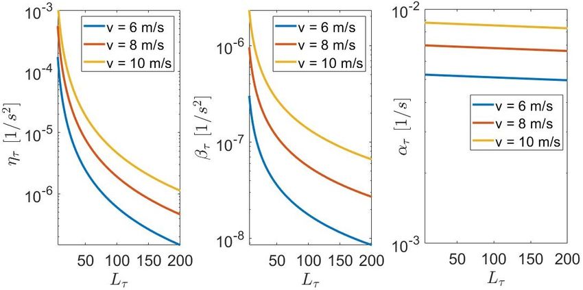
Modelling and analysis of vibrations on an aerial
cable car system with moving mass
Cesar Augusto Fonseca1 , Guilherme Rodrigues Sampaio2 , Geraldo F. de S.
Rebouças3 , Marcelo Pereira4 , and Americo Cunha Jr4
1
Centro de Instrução Almirante Wanderkolk – CIAW, Rio de Janeiro, Brazil
cesar.linhares@marinha.mil.br
2
RIO Analytics, Rio de Janeiro, Brazil
guirsp@gmail.com
3
Norwegian University of Science and Technology – NTNU, Trondheim, Norway
geraldo.reboucas@ntnu.no
4
Rio de Janeiro State University – UERJ, Rio de Janeiro, Brazil
marcelocpereira@globo.com
americo.cunha@uerj.br
Abstract. The main purpose of this work is to study the nonlinear
dynamics of an aerial cable car system. The mechanical system presented
consists of two cables, a traction cable, and a supporting cable. The
car is modeled as a concentrated mass pulled by a traction cable. The
mathematical model is described as a mass-spring system attached to a
time-varying length cable. The effects of the pulling speed shall generate
nonlinear features due to the coupling between the cable and the car and
due to external excitation.
Keywords: cable car system, nonlinear dynamics, moving boundary
problem, time-scale separation
1 Introduction
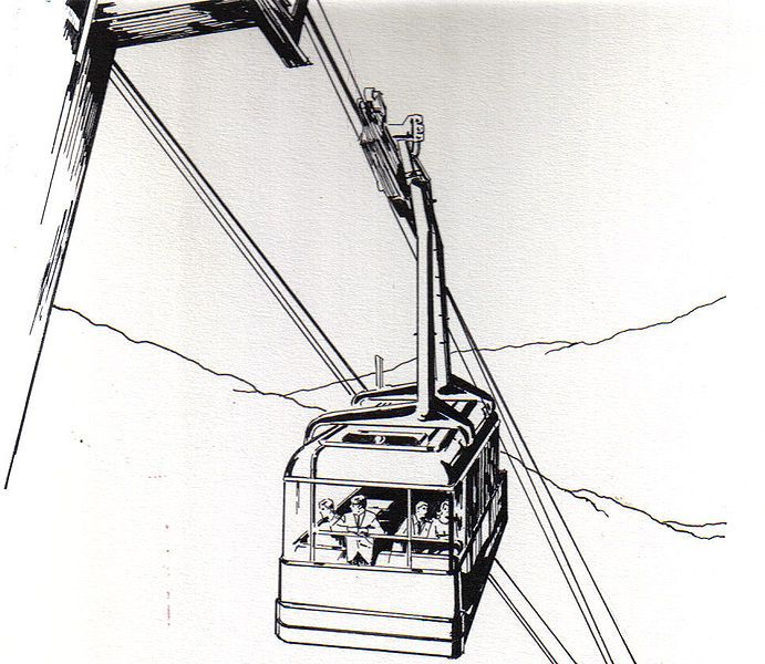
Transporting persons and items by aerial cable cars, as seen in Figure 1, has been
in use over the last hundred years for many different applications. This type of
transport is present in thousands of installations, Switzerland has alone more
than 130 in operation. The study of cable car systems is an interesting subject
in modern literature, with many different aspects of the system approached, but
published works on this topic are still only a few years old. Since it is a complex
mechanical system with many bodies, flexibility, and subject to environmental
perturbations, nonlinear phenomena may appear such as excitation of sub and
super harmonics on the cable causing vibration to the traction mechanism, which
can damage the machinery and endanger the operation.
The mechanical system studied consists of two cables, a supporting cable
fixed in both ends, and a variable-length traction cable. The car is modeled as
a concentrated mass pulled by the traction cable and connected to the support-
ing cable through a spring. In this work, we analyze the effect of vibrations in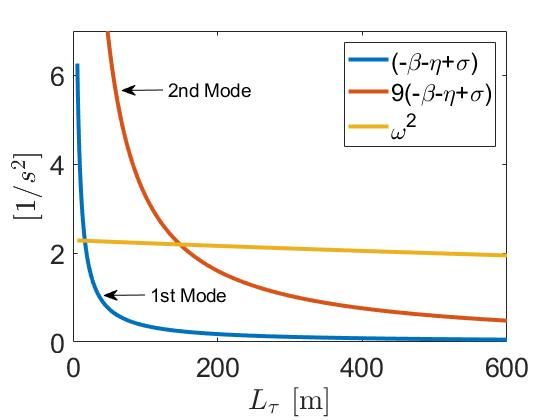
2      Fonseca et al.

            Fig. 1. Line art drawing of a typical aerial cable car system.

the traction cable according to the speed of operation and position of the car.
The coupling of the two cables and a mass-spring system creates a very com-
plex dynamic behavior that causes a nonlinear movement and can even show
some chaotic characteristics. Some references found in the literature such as the
modeling of elevators show resemblance to the present study.
    The work of Brownjohn [1] investigates the cable car that connects the is-
land of Sentosa and Singapore’s main island trough a vertical plane motion per-
spective. The article presents mathematical simulations representing the normal
operation of the system, as well as free vibration, and the situation when the
system is halted. Accelerometers measurements in the real system are used to
obtain real vibrations for each operational condition. Investigation also includes
a finite element analysis of the system followed by the results analysis.
    Terumichi et. al. [2] analyzes the non-stationary lateral vibration of a time-
varying length string with a mass-spring system guided by rail, attached to the
inferior end, a system similar to an elevator. A sinusoidal horizontal displacement
at its upper end excites the string. An analysis of the influence of the string’s
axial velocity on the vibrations is performed as well as an experimental setup
investigation. Data generated by experiment and simulation are compared.
    Bao et. al. [3] analyzes as well, a vertical motion system similar to an el-
evator, focusing on lateral vibrations of the string. In this article, the lateral
motion of the mass, coming from imperfections on the rail guide are the source
of excitation. The Hamilton principle is used to obtain the string’s equations of
motion. In the end, experimental tests results are shown and the results used
validate the numerical simulations.
    Lastly, Kaczmarczyk and Iwankiewicz [4] present a stochastic approach to
the excitation of an elevator model. The stochastic parameter are the guide rail
imperfections that excite the elevator car laterally. In order to do so, the imper-
fections are considered as a zero-mean stationary Gaussian process. Although
the model proposed in this work uses a strict deterministic approach, the knowl-
Modelling of the aerial cable car system with moving mass 3
edge on time-scale separation shown is essential for solving the problem, as seen
in another work of the same author [5].
Those works show that despite the presented cable vibration theories, there
are still very few applications to aerial cable car systems, a common system
around the world, where a failure can endanger many lives. Cable car systems
differ significantly from elevators as the gravity acts transversely to the cable.
The main originality of this work is to develop a mechanical model of a ca-
ble car system, to investigate the influence of its parameters using numerical
methods, and to explore some of its nonlinearities. The manuscript is organized
as follows: the mechanical-mathematical model for the system of interest is pre-
sented in Section 2, the numerical results, and a brief discussion in Section 3,
and finally the conclusions are made in Section 4.
2 Mechanical-mathematical model
The proposed mechanical system is illustrated in Figure 2, where a pair of over-
hung cables has a constant value of tension and is fixed on both ends with
density, circular cross-section, and constant length. The purpose of this cable is
to provide support to the cable car and to serve as the rails, where the cable
car slides on. Later, the rail cables are simplified as a single spring K attached
to the cable car represented by the concentrated mass M . The car is pulled by
another cable with a linear density ρ, cross-section A, and tension T . However,
the length of the traction cable varies in time with constant velocity v, pulling
the mass M to the origin, where the pulley is located.
Fig. 2. Schematic representation of the mechanical system used to emulate the aerial
cable car system: a variable-length cable coupled to a mass-spring oscillator.4 Fonseca et al.
To find the equivalent stiffness of the pair of supporting cables, a simple
analytical approach is used. The car passing through the extent of the supporting
cables to be simplified as a concentrated load F traveling with constant velocity,
then the solution of this problem is analytically solved and demonstrated in
Hagedorn [8]. In this case the cable deflection is given by
∞
2F L0 X 1 jπvt v jπct jπx
w(x, t) = − sin − sin sin , (1)
ρAπ 2 (c2 − v 2 ) j=1 j 2 L0 c L0 L0
p
where c = T /ρA is a constant having the dimension of speed and the product
ρA is the linear density of the cable. Then stiffness can be determined by taking
the inverse of the deflection of the supporting cables.
The analytical solution of Eq.(1) is illustrated in Figure 4 for different time
instants using the mentioned parameters. It shows the deflection of the cable at
different instants while the load moves with velocity v. The parameters used to
generate these results are shown in Table 1. The deflection of the rope reaches
its maximum value when the load is close to half of the length. Therefore, the
rail cable equivalent stiffness value is estimated as
F
K= . (2)
w(L0 /2, L0 /2 v)
The following analysis does only concern with the mass being pulled by the
cable. We begin by stating the kinetic T and the potential energy of the rope
and the mass. The total kinetic energy is
Z L(t)
1 2 1 h
2
i
T = ρ[v̇ 2 + (ẏ + v y 0 ) ] dx + M v̇ 2 + (ẏ + v y 0 ) , (3)
2 0 2 x=L(t)
and the total potential energy U is
Z L(t)
1 1
U= T y 0 2 dx + K y2 x=L(t)
. (4)
2 0 2
Here, y is the vertical displacement of the moving mass M attached to the
pulling cable with linear density ρ and constant traction T . The dot represents
the derivation in time and the ( )0 the spatial derivation.
For the traction cable, using the Hamilton principle with the adequate defi-
nition of the boundaries conditions and considering the variation of the length
gives the following initial-boundary value problem
ρ (ÿ + 2 v ẏ + v 2 y 00 ) = T y 00 , (5)
2 0 0
M (ÿ + 2 v ẏ + v y ) + K y = T y at x = L(t), (6)
y=0 at x = 0. (7)
The first boundary condition, given by Eq.(6), is not homogeneous. This term
can be transferred to the differential equation of motion, Eq.(5), by consideringModelling of the aerial cable car system with moving mass 5
the car’s dynamic forces as a concentrated load at x = L(t), rendering a simpler
and more intuitive approach [9], given by:
ρ (ÿ + 2 v ẏ + v 2 y 00 ) + 2 [M (ÿ + 2 v ẏ + v 2 y 0 + g) + K y] δ(x − L(t)) = T y 00 , (8)
y = 0 at x = 0, (9)
0
T y = 0 at x = L(t), (10)
where ẏ is the time-derivative of y, and y 0 is the corresponding spatial-derivative
with respect to x.
To promote a separation of time scales in the problem, a slow time variation
τ = ε t is introduced, in which ε = v/ω0 L0 , being ω0 is the natural frequency
of the cable without mass and spring, and L0 the maximum extent of the cable,
see [6, 7] for details.
Knowing that L(t) = L0 + v t, so, v = L̇ = ∂τ ∂L
∂t ∂τ = εν, where ν = ∂τ .
∂L
Therefore, we seek solutions of the form
N
X
y(x, t) ≈ φi (x, τ ) qi (t), (11)
i=1
where φi (x, τ ) = sin(λiτ x) and qi (t) are mode shapes and modal coordinates
associated to the underlying eigenvalue problem, respectively. The term λiτ is a
slow variation in time of the natural frequency of the cable
1 (2 i − 1) π
λiτ = . (12)
2 Lτ
Applying Eq.(11) into Eq.(8) multiplying by φj (x, τ ) and integrating between
0 and Lτ , it is possible to write the discrete dynamical equation of motion
N
X
[Mij q̈i (t) + Gij q̇i (t) + Kij qi (t)] = 0, (13)
i=1
where mass, gyroscopic and stiffness operators components are, respectively,
defined by the following expressions
Z Lτ
Mij = ρ φi φj dx + M φi (Lτ ) φj (Lτ )
0
Z Lτ
0 0
Gij = 2 ρ ν φi φj dx + 2 M ν φi (Lτ ) φj (Lτ )
0
ZLτ 0 0
Kij = ρ ν 2 2 − T φi φj dx +
0 00
M ν 2 2 φi (Lτ ) + K φi (Lτ ) φj (Lτ ). (14)
To construct the mass, gyroscopic, and stiffness matrices, the following or-
thogonality relationships are taken into account
Z Lτ Z Lτ
1 00 1
φj φi dx = Lτ δij , φj φi dx = − λ2i Lτ δij (15)
0 2 0 26 Fonseca et al.
and that
Lτ
(i − 1/2)(j − 1/2)
Z
0
φj φi dx = −2 , (16)
0 (i − 1/2)2 − (j − 1/2)2
where δij is the Kronecker delta. As seen in Blevins [10], the result from Eq.(16)
exists only when the sum i+j is odd, otherwise it is zero. Also, one has φi =
sin ( 21 (2i−1)π
Lτ x), and φj = sin ( 12 (2j−1)π
Lτ x).
Thus, for a two-mode approximation (i = 1..2 and j = 1..2) one gets
1 3
ρ Lτ + M q̈1 (t) − M q̈2 (t) + ρ ν q̇2 (t) +
2 2
1 2 2 2 1 2 2
−2 π ν ρ Lτ + M + L τ π T + 8 K L τ q1 (t) +
8 L2τ 2
1
M ν 2 π 2 2 − 4 K L2τ q2 (t) = 0,
2
(17)
4 Lτ
1 3 1
9 M ν 2 π 2 2 − 4 K L2τ q1 (t) +
ρ Lτ + M q̈2 (t) − M q̈1 (t) − ρ ν q̇1 (t) + 2
2 2 4 Lτ
1 2 2 2 1 2 2
−18 π ν ρ Lτ + M + 9 Lτ π T + 8 K Lτ q2 (t) = 0, (18)
8 L2τ 2
that can be rewritten as
q̈1 (t) − µτ q̈2 (t) + ατ q̇2 (t) + (−βτ − ητ + στ ) + ωτ2 q1 (t) +
ητ − ωτ2 q2 (t) = 0
(19)
q̈2 (t) − µτ q̈1 (t) − ατ q̇1 (t) + 9 ητ − ωτ2 q1 (t) +
9 (−βτ − ητ + στ ) + ωτ2 q2 (t) = 0,
(20)
where
1 M 3 ρν π 2 2 ν 2 ρ
mτ = ρ Lτ + M, µτ = , ατ = , βτ = ,
2 mτ 2 mτ 8 Lτ mτ
1 π 2 2 ν 2 π2 T K
ητ = 2
µτ , σ τ = , and ωτ2 = . (21)
4 Lτ 8 Lτ mτ mτ
The first term, mτ is the modal mass of the cable along with the cable car
mass, which also brings the ratio µτ of the masses. The latter couples the system
with its acceleration terms. The parameter ατ represents the Coriolis, and βτ
and ητ are the centripetal forces of the cable and the mass, respectively. The
traction can now be written as στ and the natural frequency from the attached
spring as ωτ . Each of these terms varies in the slow time τ as the pulling cable
varies its length.
3 Numerical results and discussion
By inspecting the terms in (21), as well as the Eqs.(19) and (20), it is possible
to observe the overall dependency of the cable variation in the slow time τ .Modelling of the aerial cable car system with moving mass 7
Moreover, some of them are proportional to O(1/Lτ ) like ωτ2 and ητ ; others are
proportional to O(1/L2τ ) like βτ and στ . It means that βτ , and στ can become
extremely high when the cable length is getting closer to zero. Although, the
effect is rather small for η and βτ , it is usually not for στ . It is worth pointing
out that there is a set of values in which στ surpasses the value of ωτ2 at a specific
length of Lτ .
Table 1. Parameters used to model the rail cable and the traction cable
Supporting Cables Traction Cable
Parameter Value Unit Parameter Symbol Value Unit
Linear density 39.20 kg/m Linear density ρ 3.83 kg/m
Length 600 m Initial length L0 600 m
Load 32.8 kN mass M 6550 kg
Mean Tension 10.0 kN Mean Tension T 250 kN
Velocity 6.0 m/s Stiffness K 13.4 kN/m
A numerical investigation is conducted and a set of values are given for
each of parameters from Eq.(21). Then a simulation of equations (19) and (20)
using a 4th and 5th Runge-Kutta solver is done from initial condition of a fully
extended length of cable to its almost entire retraction. The parameters used in
the simulations match the ones from a real cable car installation, meaning that
their values completely feasible and the results may represent the behavior of an
actual situation.
1s 10 s 50 s 80 s
0
-1
-2
0 200 400 600
Fig. 3. Parameter variation of the first mode in relation to the length Lτ .
Figure 4 illustrates the variation of the parameters as the traction cable
is being retracted by a constant velocity. Three different velocities are tested.
Figure 4 shows that the parameters ητ , βτ , ατ have little influence on the overall
dynamics, albeit the increase of the travelling speed.8 Fonseca et al.
When comparing the parameters στ and ωτ2 , one observes in Figure 4a that
there is a specific length of the cable that their values are equal, and as the cable
car approaches the end, στ becomes even higher that may be relevant to the
dynamics. This results in the Fig. 4b where it shows the variation of the natural
frequencies as a function of the cable length.
2
Natural
Frequencies
1.5
2nd mode
1
0.5 1st mode
0
0 200 400 600
a) b)
Fig. 4. In (a): The specific length where the natural frequencies depend more of the
cable (blue and red) than the rail stiffness (yellow). Travelling speed v = 6m/s. In (b):
Variation of the natural frequencies as function of the cable length.
To further investigate the proposed mechanical model a harmonic force is
added to the equation presented in section 2 applied to the concentrated mass M .
The nature of this force can be seen as an early approximation of the wind mean
effect acting directly on the cable-car. A Rayleigh-model damping is also included
to emulate the energy dissipation, which also prevents numerical instabilities.
A constant value for the external force frequency is chosen to be ωf = 0.26 Hz,
because it has long period time compatible to the natural behaviour of the wind.
Note in Fig. 4b that this becomes the resonance of the system twice as the cable
retracts. The result can be seen in Fig. 5, which shows the cable-car displacement
time-series y(t). As expected the cable car develops high amplitudes of oscilla-
tions twice as the cable gets shorter, and the maximum value of the amplitude
gets smaller as the travelling velocity v is higher, due to the shorter period of
time that the forcing frequency matches with one of the natural frequencies.
The presence of high amplitude oscillations shown by the numerical simula-
tion is in accordance with the real functioning cable-car seen by the maintenance
crew as it approaches the terminal station. These vibrations are mitigated by the
breaking system changing the value of the travelling speed v. Also, the model
has its own limitations, since by shortening the cable means that the mass M is
reaching its boundary condition, which would lead to numerical instabilities or
misrepresentation of the real phenomena.Modelling of the aerial cable car system with moving mass 9
1 1 1
0.5 0.5 0.5
0 0 0
-0.5 -0.5 -0.5
-1 -1 -1
0 200 400 600 0 200 400 600 0 200 400 600
1 1 1
0.5 0.5 0.5
0 0 0
-0.5 -0.5 -0.5
-1 -1 -1
0 200 400 600 0 200 400 600 0 200 400 600
Fig. 5. Displacement for different velocities v of the cable-car when the system is
excited by a harmonic force at F (t) = 300 sin (ωf t) [N] at x = Lτ .
4 Conclusions and future perspectives
This work presented a mechanical-mathematical model for a cable car system.
First, the equations of motion are developed, and numerical analysis is conducted
with parameters inspired by a real case. This analysis shows the changes of each
parameter as a function of the cable length, among them the increase of the
stiffness parameter related to the cable.
This paper paves the way for a series of different analysis, which may include
the variation of the stiffness parameter related to the pair of supporting cables,
the investigation of the influence of a harmonic forcing at the origin, which would
represent the machinery responsible for actuating the whole system.
Results show that some points of the trajectory and some speeds present
higher amplitude vibrations than others, this is an important non-linear phe-
nomenon that poses challenges to the operation of systems similar to the one
modeled. The understanding of those phenomena, as well as its numerical mod-
eling, is of high importance to the safe operation of aerial cable cars.
Another possibility is to include the presence of a random force concentrated
at the mass, representing the wind or passengers moving inside the car. Lastly,
these models can be compared to other numerical analyses with finite elements
models or even with experimental data. This research can also be adapted to
other mechanical equivalent found in installations such as in ski lifts.10 Fonseca et al. Acknowledgments The fourth author would like to thank the financial support given to this research by the Brazilian agencies Coordenação de Aperfeiçoamento de Pessoal de Nı́vel Superior - Brasil (CAPES) - Finance Code 001, and the Carlos Chagas Filho Research Foundation of Rio de Janeiro State (FAPERJ) under the following grants: 211.304/2015, 210.021/2018, 210.167/2019, and 211.037/2019. References 1. Brownjohn, J.M.W.: Dynamics of an Aerial Cableway System, Engineering Struc- tures, Vol. 20, No. 9, pp. 826-836. (1998) 2. Terumichi, Y., Ohtsuka, M., Yoshizawa, M., Fukawa, Y. and Tsujioka, Y.: Nonsta- tionary Vibrations of a String with Time-Varying Length and a Mass-Spring System Attached at the Lower End, Nonlinear Dynamics, Vol. 12, pp 39-55. (1997) 3. Bao, J., Zhang, P. and Zhu, C.: Dynamic Analysis of Flexible Hoisting Rope with Time-Varying Length, International Applied Mechanics, Vol. 51, No. 6, pp. 710-720. (2015) 4. Kaczmarczyk, S., Iwankiewicz, R.: Dynamic response of an elevator car due to stochastic rail excitation, Proceedings of the Estonian Academy of Sciences, Vol. 55, No. 1, pp. 58-67. (2006) 5. Kaczmarczyk, S.: The passage through resonance in a catenary–vertical hoisting cable system with slowly varying length, Journal of Sound and Vibration, Vol. 208, No. 2, pp. 243-269. (1997) 6. Cunha Jr.,A., Fonseca, C.A., Rodrigues, G. and Pereira M., Analysis of Vibrations on an Aerial Cable Car System With Moving Mass, Proceedings of the XV Inter- national Symposium on Dynamic Problems of Mechanics, DINAME 2019, Buzios, RJ, Brazil, March 10th to 15th , 2019 7. Colón,D., Cunha Jr,A., Kaczmarczyk, S., Balthazar, J., On dynamic analysis and control of an elevator system using polynomial chaos and Karhunen-Loève ap- proaches, Procedia Engineering 199, pp. 1629–1634 (2017) 8. Hagendorn, P.: Nonlinear Oscillations, Oxford Sci. Publ., Oxford. (1988) 9. Meirovitch, L.: Fundamentals of Vibrations, McGraw-Hill, New York. (2000) 10. Blevins, R.D.: Flow-induced Vibration, Van Nostrand Reinhold, (1990)
You can also read