Models of Ponding In Two Flooded Recharge Basins
←
→
Page content transcription
If your browser does not render page correctly, please read the page content below
Models of Ponding In Two Flooded Recharge Basins
Abstract
        Groundwater recharge basins are the primary method of managing stormwater runoff on
Long Island. Many of the basins excavated on the Ronkonkoma and Harbor Hill moraines
contain standing water, and do not drain (Aronson and Seaburn). The interest of this study is a
system of connected recharge basins that are perpetually flooded. The basins receive a constant
input of industrial cooling and leak water, in addition to stormwater from paved surfaces over a
large portion of Stony Brook University's West campus. Initial investigations indicated that the
basins might intersect a groundwater mound (Tuomey). In this study, several scenarios were
modeled using Visual MODFLOW and MOUNDHTsoftware. Researchers also collected well
data and took sediment samples, which assisted in calibrating the models. A better
understanding of the hydrogeologic framework of the basins as well as subsurface stratigraphy is
important for understanding the management of stormwater systems.

Introduction
         The residents of Nassau and Suffolk counties rely on groundwater from unconfined
aquifers as a sole source of water (Oliva). In order to ensure a sufficient supply of fresh water
reaches the aquifer, the use of conservative mesures, such as artificial recharge basins, is
necessary. In addition to providing recharge to the aquifer, artificial recharge basins are an
effective means of managing stormwater runoff in urbanized areas (Aronson, 1979).
         Many artificial recharge basins on Long Island contain standing water. Standing water in
recharge basins can be caused by clogging, which is the accumulation fine sediments and organic
matter on the basin floor (Aronson and Seaburn). They may also be flooded, due to intersection
of the water table (Aronson and Seaburn), intersection of a perched water table (Aronson and
Seaburn), placement in deposits of low hydraulic conductivity (Aronson and Seaburn), or due to
intersection of a groundwater mound formed by a high inflow of water into the recharge basin
(Fig. 1) (Pizzuli). Flooded basins drain directly into the saturated zone, since there is no
intervening unsaturated zone between the water in the basins and the water table. Since the
hydraulic gradient between flooded basins and the water table is small, flooded basins drain
slowly (Aronson).
         The basins on the northwest side of
Stony Brook University's West Campus (Fig.
2) are continually flooded. In at least one
past occasion, the basins overflowed,
damaging the nearby Long Island Rail Road
tracks, as well as several residential properties
along State Route 25A.
         Groundwater mounding (fig. 1) is the
rise of the local water table in response to
excessive recharge (Fetter). Mounding
appears on water table contours in a similar
fashion to the way a hill would look on a
                                                  Figure 1: Flow of water from a recharge basin
surface elevation contour map. Mounding is through the unsaturated zone, after Pizzulli (1999).
                                                                                          Page 1 of 23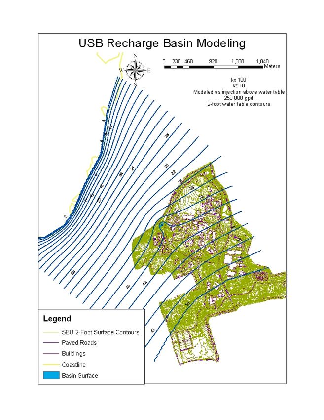
Nicholas D. Kilb (100882207)                                        Geology Department
SUNY at Stony Brook, Fall 2005                                      Undergraduate Research Report
                                                         typical under storm water and wastewater
                                                         recharge basins. Typical mounding
                                                         under stormwater basins on Long Island
                                                         ranges from one to six feet after storm
                                                         events (Haskell and Bianchi). The basins
                                                         on the northwest side of Stony Brook
                                                         University's West Campus (Fig. 2) are
                                                         unique in that they receive a constant
                                                         influx of water from cooling and leaks,
                                                         and an episodic influx due to storm
                                                         water. This means the average inflow to
                                                         the basins is 100,000-500,000 gallons per
                                                         day (Rispoli). This large amount of
                                                         water must flow out of the basins to
                                                         prevent them from overflowing. The
                                                         average hydraulic conductivity of the
                                                         sediments in the area is quite low, since
Figure 2: Area map for the project. The study area is   there are many layers of glacial clay and
highlighted in red.                                   silt in the sediments beneath the basins.
Therefore, the water escapes the basins slowly, and exacerbates the local mounding effect.
        We have a poor understanding of the stratigraphy beneath the basins. A clay lens was
encountered at an elevation of 50', when a well was drilled 45' north of the northernmost basin
(Basin 1). Based on the texture and color of the clay, and the stratigraphy of the region, it could
be a lens of the Smithtown Clay, which has been observed nearby in Nissequogue (Krulikas and
Koszalka). Glacial tectonics has strongly influenced this area, and the clay lens underlying the
basins, it may be dipping, or may terminate abruptly. The modeling in this study did not
consider the clay, due to limited knowledge of the stratigraphy of the area, including the spatial
extents and orientation of the clay lens.
        The purpose of this experiment was to model the effects of groundwater mounding on the
elevation of the water table on Stony Brook's West Campus (fig. 2), and relate it to the elevation
of standing water in the recharge basins. I made several maps with potential water table contours
using groundwater-modeling software in conjunction with Geographic Information System (GIS)
software (ArcGIS). Groundwater mounding underneath the recharge basins may cause slower
drainage in the basins, and in some cases, the mounds may intersect the basins, causing them to
be perpetually flooded. My hypothesis is that groundwater mounding significantly alters
groundwater flow in the local area, and prevents the basins from properly draining.

Methods
        A conceptual model was designed based on the potential inputs and outputs for the
basins, and potential causes for the standing water. A research group then collected sediment
samples from the bottom of one of the basins, to evaluate clogging as a potential cause of the
standing water. Next, a separate research group collected well data and standing water

                                                                                      Page 2 of 23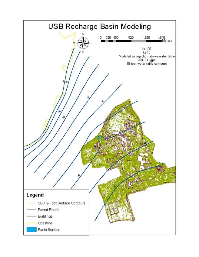
Nicholas D. Kilb (100882207)                                         Geology Department
SUNY at Stony Brook, Fall 2005                                       Undergraduate Research Report
elevations. Finally, the data was combined with pulished data in the creation of a groundwater
model and subsequent sensitivity analysis using Visual MODFLOW 4.1.
        The sediment samples were collected by a team using a rowboat, a grab sampler, several
grab sample coring tubes, and several whirl-pak bags. We collected the sediments from Basin 2,
which is the middle basin in the 3-basin complex, on November 10, 2005. Sediments had been
collected in Basin 1 during an earlier experiment (Pizzuli). Basin 2 is a man-made basin that was
constructed in a glacial tunnel valley (Hanson, July 2005). Basin 2 is excavated in a deposit of
primarily coarse sand and gravel, and it had been expanded and scarified approximately 6
months prior to the sampling (Rispoli). The water level in the basin was 14 feet ± 1 foot,
according to the gauge pole on the day of sampling.
        In order to measure the extent of the mounds, we collected data on the elevations of
several monitoring wells in the area. We also measured the elevation of the surface water level
in the two basins that contain standing water (Basin 1 to the north, and Basin 2 in the middle of
the three basins). For this task, we used the technique of differential leveling. In differential
leveling, one uses a level to sight a measuring stick. The height of the level is first determined
by referencing the level to a point of known elevation, in this case the floor of the Stony Brook
West Campus Heating Plant. Next, one measures the elevation of other points of interest relative
to the level. This gives the elevation relative to the level, which one can then relate back to the
reference point. At that point, we may move the level and reference it to the points that we
measured the elevation of. We continue in that fashion until we have referenced all points of
interest.
        The group also measured depth to water and depth to bottom in the wells for which we
had measured the surface elevations. We accomplished this with a weighted steel tape. We
lowered the tape into the well until we were confident it was below the water table. We recorded
the depth of the tape we lowered down the well by reading it against the well's edge. Next, we
raised the tape and recorded the location of the water table in relation to the tape by noting where
the tape was wet. By subtracting the relative location of the water table from the depth to which
we lowered the tape, we arrived at the depth to water. We subtracted the depth to water from the
well's elevation to obtain the elevation of the water table.
        GIS is a computer tool for making maps containing various layers of geographic data.
This enables all or just selected portions of the data to be displayed on a map in a number of
ways. We used ArcGIS version 9.1 for Windows PCs, published by ESRI, Inc. We used
existing GIS shapefiles to display surface elevation contours, buildings, roads, well locations
(Kilb, "Groundwater Mapping"), and basin locations (based on contour data) on the map. We
drew a shapefile of approximate water table contours based on the well data by "heads-up
digitizing." This map was compared to the models, as a quick method of testing their
predictions.
        In order to model the extent of the mounds, I used published data concerning the regional
hydrology of northern Brookhaven township (Jensen; Koszalka 1980; Olanrewaju) to construct a
regional flow model (Figure 3, Appendix A), using Visual MODFLOW 4.1. This flow model
assumed a vertical hydraulic conductivity of 230 feet per day, and a horizontal hydraulic
conductivity of 23 feet per day. The model's boundary conditions were set to a constant-head
boundary at the 50-foot regional water table contour on the current USGS regional water table
contour map (Busciolano), and a constant-head boundary of 0' according to a map of the Long
                                                                                         Page 3 of 23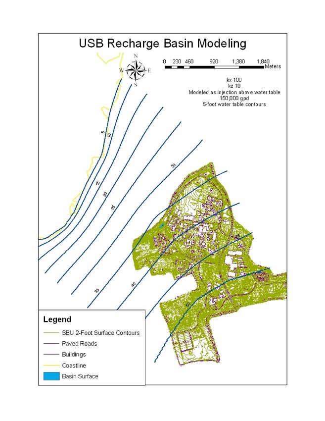
Nicholas D. Kilb (100882207)                                                   Geology Department
SUNY at Stony Brook, Fall 2005                                                 Undergraduate Research Report
Island coastline. The regional flow model was set to run until a steady state was reached, after
approximately 10 years. Once a regional flow model was created, several scenarios were tested
by varying conductivity values, conductance of the beds of the basins, and the volume flux of
water through the basins.
Results and Discussion
         Fine sediments in Basin 2 ranged in thickness from less than 1 mm on the northeastern
side, near the gauging pole, to approximately 5 cm in the center. The sediments appeared to be
stratified in 4 layers, perhaps indicating storm events. The lowest layer appeared to consist of a
light-colored silt. The next layer was thicker, and was composed of dark, cohesive, possibly
organic-rich sediment. The next layer resembled a grey clay, and the last layer was made up of
loosely bound organic matter, mostly leaf litter. Results from Basin 1 (Maher) indicated that the
sediments on the bottom of Basin 1 were between 5 cm and 13 cm thick.
         The mapping group began by mapping the elevations of several monitoring wells near the
West Campus Heating Plant. We had previously measured the elevations for a Field Geology
class, (Kilb, "Groundwater Mapping"), but we desired better closure. Our calculated closure for
those wells was 0.573m. This is a good closure compared to previous results.
         We then took elevations of several landmarks (light poles and fence posts) as
intermediate reference points. Along the way, we took several intermediate closures, all of
which were small. We used the intermediate points to measure the elevation of the well near
Basin 1, and the surface water in the Basin 1 and Basin 2. Table 1 summarizes the results. All
elevations are in feet.
Table 1: Depth to water and elevation of the water table for the wells.
                         De pth to W a te r (ft)                      Ele va tion (ft)
Trial Number             B1 MW MW 2              MW 3        MW 8     B1 MW MW 2           MW 3      MW 8
                     1    44.417 67.20833           70.875    70.19792 51.539 39.03896      39.27333 39.04938
                     2    44.083 67.20833 71.01042            70.17188 51.872 39.03896      39.13792 39.07542
                     3    44.813                  70.99479             51.143               39.15354
                     4    44.813                                       51.143
                     5       44.5                                      51.456
Top of W ell                    0            0           0           0 95.956 106.2473     110.1483 109.2473
Bottom of W ell           50.063                                       45.893
Average W ater Table      44.525 67.20833 70.96007             70.1849 51.431 39.03896     39.18826  39.0624
Standard Deviation        0.3053             0 0.074085       0.018414 0.3053          0   0.074085 0.018414
        Note that in table 1, I calculated the elevation of the bottom of the basins. The basins do
not have flat, uniform bottoms, and the elevations shown indicate the deepest portions of the
basins. I based elevation of the bottom of Basin 1 on a gauging pole installed in the basin, which
is accurate to within a foot, based on prior studies. I based the elevation of the bottom of Basin 2
on a bathymetric study performed by Michelle E. Pizzulli (Pizzulli 1999).
        Next, we calculated the depth to water in the wells (Table 2, Appendix A). Due to
difficulty in measuring, we took several readings for each well. I have displayed the average and
standard deviation for the measurements at each well. I used the average values along with the
elevation values to calculate the elevation of the water table. The elevation of the water in the
well near Basin 1 is of particular interest. The water table at that point is only one meter below

                                                                                                  Page 4 of 23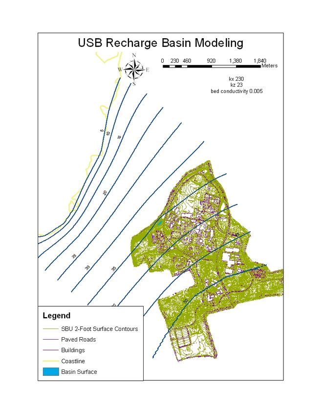
Nicholas D. Kilb (100882207) Geology Department
SUNY at Stony Brook, Fall 2005 Undergraduate Research Report
the elevation of the deepest part of Basin 1, so I expect that the water table may intersect the
bottom of the basin.
Figure 4 (Appendix A) shows the estimated water table contour map created in ArcGIS.
The regional water table should be at an approximate elevation of 35 feet, and regional flow
should be to the northwest. Note that the estimated contours indicate that local flow seems to
radiate outward from the basins.
The first series of models of the recharge basins tested whether uncertainty in the
horizontal and vertical hydraulic conductivities of the aquifer material in the area would
significantly influence drainage patterns from the basins. The model was also used to determine
the maximum amount of mound growth that could occur beneath the basins, for a given value of
the hydraulic conductivity of the sediments on the basin floors.
Figures 5-9 (Appendix A) show the results of models assuming typical conductivity
values for the Upper Glacial aquifer (Jensen; Koszalka 1980; Olanrewaju). Next, and an
unlimited input was allowed to the basins, so that the maximum extent of the mound could be
observed, if clogging due to aquifer conductivity or basin floor sediments was limiting. This was
obtained by treating the basin as a stretch of river, using the river package in Visual
MODFLOW. The thickness of basin floor sediments was input based on observations in the
sediment study. Figures 5-8 display the results of models assuming that the conductivity of the
basin floor sediments is 0.5, roughly the equivalent of fine clay (Fetter). Note that aquifer
conductivity values are in no case limiting, since these models all produce identical results,
despite variation within acceptable ranges for horizontal and vertical hydraulic conductivities.
Based on this assessment, vertical and horizontal hydraulic conductivities were not varied after
this point. Assuming that the basin floor sediments are composed of fine clay the basins would
still be fairly permeable, and steady state mounding as high as 73 feet could occur. Figure 9
displays the results of a model assuming that the conductivity of the basin floor sediments is
0.005, roughly the equivalent of concrete (Fetter). Note that some steady state mounding could
still occur in this case, although it is unlikely that bed conductivities would be so low.
Figures 10-14 show the results of models assuming acceptable conductivity values for the
Upper Glacial aquifer, with a horizontal conductivity value of 100 feet per day, and vertical
conductivity of 10 feet per day. In these cases, conductivity of the basin floor was disregarded.
Instead, volume flux through the basins was considered. This was accomplished by modeling
the basins as two injection wells screened above the water table using the injection well package
in Visual MODFLOW, and varying the rate of injection, based on estimated values of steady
input to the basins. Figure 10 displays the results of mounding under the basins for 150,000
gallons per day, which is the minimum value of cooling and leak water entering the basins,
estimated based on discussions with Bruno, Lefferts, and Rispoli. Such a case would result in
steady state mounding of approximately 3' at the maximum. Figures 11 and 12 display the
results of mounding under the basins for 250,000 gallons per day, which is a conservative mid-
range estimate of cooling and leak water entering the basins, based on discussions with Bruno,
Lefferts, and Rispoli. Such a case would result in steady state mounding of approximately 7' at
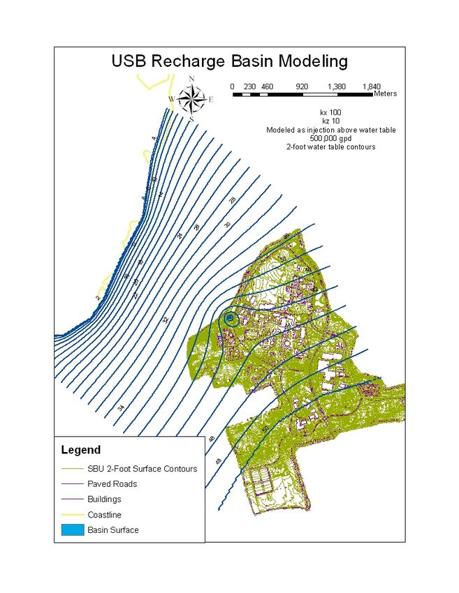
the maximum. Figures 13 and 14 display the results of mounding under the basins for 500,000
gallons per day, which is a conservative mid-range estimate for the combination of stormwater
runoff and cooling and leak water entering the basins, based on discussions with Bruno, Lefferts
and Rispoli, along with Pizzuli's estimates of runoff from paved surfaces minus infiltration.
Page 5 of 23
Nicholas D. Kilb (100882207)                                         Geology Department
SUNY at Stony Brook, Fall 2005                                       Undergraduate Research Report
Such a case would result in steady state mounding of approximately 17' above the regional water
table at the maximum, resulting in a water table elevation of 52'.

Conclusions
        Groundwater flow on the northwest part of Stony Brook campus is strongly influenced by
recharge mounding under the recharge basins located there. A groundwater mound with a
maximum elevation of at least 51.43 feet exists below Basin 1, based on well data. Modeling
predictions of a steady-state groundwater mound based on reasonable basin bed sediment
conductivity values, and reasonable estimates for the daily flux of water through the system,
arrive at similar results (Fig. 14).
        It is not likely that clogging hinders the draining of the basins. Based on basin bed
sediment profiles, estimated conductivity values (Figs. 5-9), and well data (Fig. 4), it is unlikely
that clogging is causing the basins to remain flooded, given the size of the mound that is present.
        A clay layer may reside beneath the basins, which could cause a perched water table to
form, rather than a mound. This would significantly increase the maximum height of the water
table, possibly causing the basins to flood to their current levels of standing water. Further
investigations, including vibrocore drilling and possibly "Chirp" seismic profiling of the basins is
recommended.
        It is possible that the basins are flooded due to a combination of mounding, clogging, and
large, continuous inputs of water to the basins. Mounding would, at the least, decrease pore
pressures in the unsaturated zone, and if the mounds intersected the basins, then there would be
no unsaturated zone, and drainage would be severely limited (Aronson and Seaburn).

Recommendations
         Several engineering practices have been employed to allow the basins to drain better.
First, the basins have been routinely scarified to eliminate clogging by fine particulate matter.
Scarifying is the process of removing fine-grained material, exposing the sandy-gravelly
sediment underlying the basins (Aronson and Seaburn).
         A retention basin system (Fig. 15) was inherent in the design of the basins, although that
system has since been modified. Retention basins management involves the use of several
basins. All runoff is
input to the first basin,
where sediment is
allowed to settle over a
period of time. A pipe
connects the top of first
basin to the second basin,
allowing sediment-free
overflow to spill into the Figure 15. Diagram of a Retention Basin management system. After
                             Aronson and Seaburn.
second basin, where it
should be readily able to drain. Originally, the basins on the northwest side of Stony Brook
University's West Campus were arranged in this fashion, with all runoff entering Basin 1, and
only overflow entering Basin 2. Several construction projects (construction of the West
                                                                                        Page 6 of 23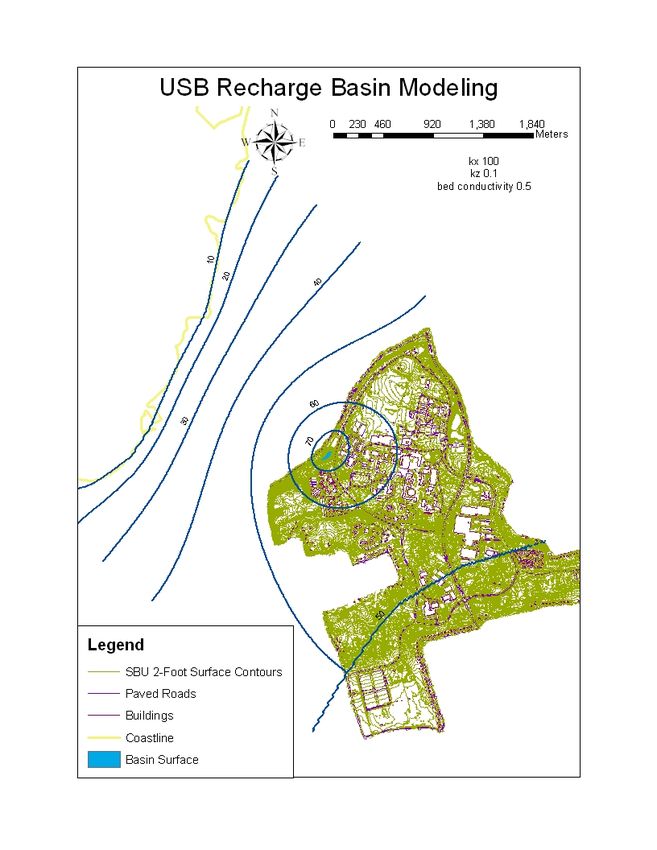
Nicholas D. Kilb (100882207)                                           Geology Department
SUNY at Stony Brook, Fall 2005                                         Undergraduate Research Report
Apartments, and several road maintenance programs) have diverted runoff directly to Basin 2,
causing silting to occur, as evidenced by the sediment survey.
         Based on the bathymetry of the basins (Pizzuli), it appears that auxiliary infiltrating areas
(Fig. 16) have been
employed. The purpose
of auxiliary infiltrating
areas is to allow
sediment-laden water to
enter the basin, and settle
in a deeper part of the
basin that is wet more
frequently. If that area
becomes clogged, the
water level will rise, and
the overflow will spill
                               Figure 16. Diagram of an Auxiliary Infiltrating Area management system.
over the unclogged,            After Aronson and Seaburn.
auxiliary infiltrating area,
allowing the water to
infiltrate (Aronson and Seaburn). Currently, the auxiliary infiltrating areas are submerged, and
the full extent of the basin is subject to silting.
         Recently, fourteen diffusion wells were installed, when Basin 2 was scarified (Rispoli).
Diffusion wells are sometimes used to
combat clogging, although in areas
prone to clogging, the diffusion wells
become clogged and cease to function
rather quickly (Aronson and Seaburn).
More often, diffusion wells are used in
basins that are placed above deposits of
low hydraulic conductivity, such as clay
lenses (Fig. 17). Diffusion wells consist
of several concrete infiltration rings that
are buried to a level below the deposits
of low hydraulic conductivity, and then
capped by a sand and gravel filter pack,
to prevent silt from entering the wells.
The wells installed in Basin 2 consist of
two 8' concrete rings, which are buried
to a depth of 12' below the basin floor
(and elevation of 53', which is 2' above
the elevation of the top of the clay layer
found in the monitoring well), and 4'
above the basin floor. They are fitted at Figure 17. Diagram of an Diffusion Well management
the top by large metal gratings, and           system. After Aronson and Seaburn.

                                                                                         Page 7 of 23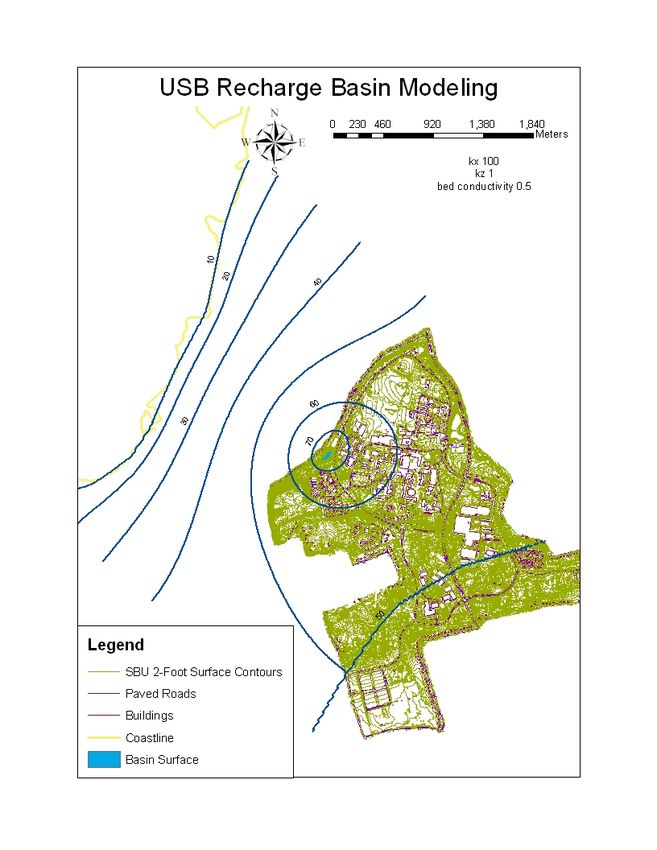
Nicholas D. Kilb (100882207)                                        Geology Department
SUNY at Stony Brook, Fall 2005                                      Undergraduate Research Report
have not been covered with filter packs. Currently, ten of the diffusion wells are fully
submerged.
         I recommend that any future stormwater runoff be diverted to Basin 1, to maximize the
usage of the Retention Basin management plan. Further, I recommend that future construction
budgets for the basins include stratigraphic analysis of the underlying sediments, to determine if
infiltration is being limited by deposits of low hydraulic conductivity. If this is the case, I
recommend that diffusion wells be installed to a depth well below the deposits, and that they be
covered by a sand and gravel filter pack, to prevent silt clogging within the concrete rings.

                                                                                      Page 8 of 23
Nicholas D. Kilb (100882207)                                      Geology Department
SUNY at Stony Brook, Fall 2005                                    Undergraduate Research Report
References
ArcGIS 9.0. Computer Software. ESRI, 2004.
Aronson, D.A. "Use of storm-water basins for artificial recharge with reclaimed water, Nassau
        County, Long Island, New York: a hydraulic feasibility study." Long Island Water
        Resources Bulletin no. 11, 57 pages. 1979.
Aronson, D.A. and Seaburn, G.E. "Appraisal of Operating Efficiency of Recharge Basins on
        Long Island, New York, in 1969." USGS Water Supply Paper 2001-D. Washington,
        D.C. 1974.
Bruno, P. Personal interview. SUNY at Stony Brook, New York. Fall 2005.
Busciolano, R. "Water-Table and Potentiometric-Surface Altitudes of the Upper Glacial,
        Magothy, and Lloyd Aquifers on Long Island, New York, in March-April 2000, with a
        Summary of Hydrogeologic Conditions: Second Edition." USGS Water-Resources
        Investigations Report 01-4165. Coram, New York. 2002.
Fetter, C.W. Applied Hydrogeology, 4th Edition. Upper Saddle River, NJ: Prentice Hall.
        598 pages. 2001.
Hanson, G.N. Personal conversations. SUNY at Stony Brook, New York. Fall 2005.
Hanson, G.N. "Glacial Geology of the Stony Brook-Setauket-Port Jefferson Area." Long Island
        Geology Research Papers on the Web. July 13, 2005. April 21 2006.
        < http://pbisotopes.ess.sunysb.edu/reports/dem_2/index.htm>
Haskell, E.E., Jr., and Bianchi, W.C. "Decelopment and Dissipation of Groundwater Mounds
        Beneath Square Recharge Basins." American Water Works Association Journal vol. 57,
        no. 3, p. 349-353. 1965.
Jensen, H.M. "Hydrogeology of Suffolk County, Long Island, New York." USGS Hydrologic
        investigations atlas HA-501. Washington, D.C. 1974.
Kilb, N. "Mapping Bodies of Water on Stony Brook Campus." GEO 305: Field Geology Course
        Work. SUNY at Stony Brook, New York. September 2005.
Kilb, N. "Groundwater Mapping." GEO 305: Field Geology Course Work. SUNY at Stony
        Brook, New York. September 2005.
Kilb, N. "Optional Report." GEO 305: Field Geology Course Work. SUNY at Stony Brook,
        New York. December 2005.
Kilb, N. "Recharge Basin Field Trip." Proc. of Geology of Long Island and Metropolitan New
        York Conf., 22 Apr. 2006, SUNY at Stony Brook, New York.
Koszalka, E.J. "Hydrogeologic data from the northern part of the town of Brookhaven, Suffolk
        County, New York." Long Island Water Resources Bulletin no. 15, 80 pages. 1980.
Krulikas, R.K. and Koszalka, E.J. "Geologic Reconnaissance of an Extensive Clay Unit in
        North-Central Suffolk County, Long Island, New York." U.S.G.S. Water-Resources
        Investigation Report: 82-4075 Coram, New York. 1983.
Lefferts, R. Personal interviews. SUNY at Stony Brook, New York. Fall 2005.
Maher, N. Personal conversations. SUNY at Stony Brook, New York. Fall 2005.
Misut, P. Personal conversations. USGS Water Resources Division, Field Office, Coram, New
        York. Fall 2005.
Olanrewaju, J.N. "Hydraulic conductivity, porosity, and particle size distribution of core
        samples of the upper glacial Aquifer: laboratory observations: a final report." Research

                                                                                    Page 9 of 23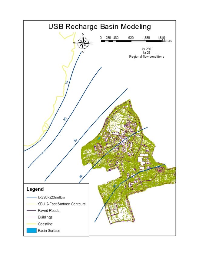
Nicholas D. Kilb (100882207)                                     Geology Department
SUNY at Stony Brook, Fall 2005                                   Undergraduate Research Report
        Report: Stony Brook, N.Y.: State University of New York at Stony Brook, Dept. of Earth
        and Space Sciences. 50 pages. 1994.
Oliva, James A. "Operations at the Cedar Creek Wastewater Reclamation-Recharge
        Facilities, Nassau County, New York." In Asano, Takashi, (ed.), Artificial Recharge
        of Groundwater: London, Butterworth Publishers, p.397-424. 1985.
Pizzulli, M.E. "Fate of Nitrogen in a Ponded Recharge Basin." Proc. of Geology of Long Island
        and Metropolitan New York Conf., 24 Apr. 1999, SUNY at Stony Brook, New York. 18
        December 2005. .
Rispolli, L. Personal interviews. SUNY at Stony Brook, New York. Fall 2005.
Tuomey, A.M.
Visual MODFLOW 4.1. Computer Software. Waterloo Hydrogeologic Inc., 2005.

                                                                                  Page 10 of 23
Nicholas D. Kilb (100882207) Geology Department
SUNY at Stony Brook, Fall 2005 Undergraduate Research Report
Appendix A: Modeling Results
Figure 3. Initial model of regional flow conditions, assuming standard conductivities for
the Upper Glacial aquifer: horizontal conductivity of 230 feet per day, vertical conductivity
of 23 feet per day, and with no input from the recharge basins.
Page 11 of 23Nicholas D. Kilb (100882207) Geology Department
SUNY at Stony Brook, Fall 2005 Undergraduate Research Report
Table 2: Elevation data for the wells and recharge basins.
Point from Point to Foreshot (ft) Backshot (ft) Elevation (ft) Closure (ft) Description
Building Map 106.94 NA Heating Plant floor elevation
1 Building 5.21354167 112.1535417 NA HI at Point 1
1 MW3 2.00520833 110.1483333 0 Flush Mount Well
1 MW2 5.90625 106.2472917 0 Stand Pipe Well in Lawn
1 MW8 2.90625 109.2472917 0 Stand Pipe in Parking Lot
2 Building 2.29166667 109.2316667 NA HI at Point 2
2 MW2 2.92708333 106.3045833 0.0572917 Stand Pipe Well in Lawn
2 LP1 7.05208333 102.1795833 - Light Pole near basins
3 LP1 3.5625 105.7420833 NA HI at Point 3
3 LP2 7.14583333 98.59625 - Next Light Pole NE of LP1
4 LP1 0.28125 102.4608333 NA HI at Point 4
4 LP2 3.82291667 98.63791667 0.0416667 Next Light Pole NE of LP1
4 LP3 6.45833333 96.0025 Next Light Pole NE of LP2
4 L B2 GP 7.5625 94.89833333 - Left Basin 2 Gate Post
4 R B1 GP 7.66666667 94.79416667 - Right Basin 1 Gate Post
5 R B1 GP 0.22916667 95.02333333 NA HI at Point 5
5 AP1 8.5625 86.46083333 - Arbitrary Point 1
6 AP1 0.484375 86.94520833 NA HI at Point 6
6 B1 WL 6.96875 79.97645833 - Water Level in Basin 1
7 LP2 1.56770833 100.1639583 NA HI at point 7
7 LP3 4.14583333 96.018125 0.015625 Next Light Pole NE of LP2
7 B1 MW 4.20833333 95.955625 - Monitoring Well near Basin 1
8 L B2 GP 0.72916667 95.6275 NA HI at Point 8
8 AP2 8.36979167 87.25770833 Arbitrary Point 2
9 AP2 0.15625 87.41395833 HI at Point 9
9 B2 WL 7.63020833 79.78375 Water Level in Basin 2
9 Pole 22 65.41395833 Bottom of basin 2, according to Gauge Pole
Pole B2 WL 14.3333333 79.74729167 0.0364583 Water Level in Basin 2
B1 WL B1 Bottom 27 52.97645833 Bottom of Basin 2, according to Pizzuli
Page 12 of 23Nicholas D. Kilb (100882207) Geology Department
SUNY at Stony Brook, Fall 2005 Undergraduate Research Report
Figure 4: Contour map of Stony Brook Campus, with overlay of shapefiles based on the
mapping data in table 1 and water table contours based on the well data in table 2. Page 13 of 23Nicholas D. Kilb (100882207) Geology Department
SUNY at Stony Brook, Fall 2005 Undergraduate Research Report
Figure 5: 10' interval water table contours, assuming standard conductivities for the
Upper Glacial aquifer: horizontal conductivity of 230 feet per day, vertical conductivity
of 23 feet per day, unlimited flow into the basins, and with conductivity of basin floor
sediments of 0.5 feet per day.
Page 14 of 23Nicholas D. Kilb (100882207) Geology Department
SUNY at Stony Brook, Fall 2005 Undergraduate Research Report
Figure 6: 10' interval water table contours, assuming local conductivities for Upper
Glacial aquifer: horizontal conductivity of 100 feet per day, vertical conductivity of 1 foot
per day, unlimited flow into the basins, and with conductivity of basin floor sediments of
0.5 feet per day.
Page 15 of 23Nicholas D. Kilb (100882207) Geology Department
SUNY at Stony Brook, Fall 2005 Undergraduate Research Report
Figure 7: 10' interval water table contours, assuming local conductivities for Upper
Glacial aquifer: horizontal conductivity of 100 feet per day, vertical conductivity of 0.1
feet per day, unlimited flow into the basins, and with conductivity of basin floor
sediments of 0.5 feet per day.
Page 16 of 23Nicholas D. Kilb (100882207) Geology Department
SUNY at Stony Brook, Fall 2005 Undergraduate Research Report
Figure 8: 10' interval water table contours, assuming local conductivities for Upper
Glacial aquifer: horizontal conductivity of 20 feet per day, vertical conductivity of 2 feet
per day, unlimited flow into the basins, and with conductivity of basin floor sediments of
0.5 feet per day.
Page 17 of 23Nicholas D. Kilb (100882207) Geology Department
SUNY at Stony Brook, Fall 2005 Undergraduate Research Report
Figure 9: 5' interval water table contours, assuming standard conductivities for Upper
Glacial aquifer: horizontal conductivity of 230 feet per day, vertical conductivity of 23
feet per day, unlimited flow into the basins, and with conductivity of basin floor
sediments of 0.005 feet per day.
Page 18 of 23Nicholas D. Kilb (100882207) Geology Department
SUNY at Stony Brook, Fall 2005 Undergraduate Research Report
Figure 10: 5' interval water table contours, assuming acceptable conductivities for Upper
Glacial aquifer: horizontal conductivity of 100 feet per day, vertical conductivity of 10
feet per day, and a flow out of the basins of 150,000 gallons per day. The center of the
mound is approx. 3' higher than the regional water table.
Page 19 of 23Nicholas D. Kilb (100882207) Geology Department
SUNY at Stony Brook, Fall 2005 Undergraduate Research Report
Figure 11: 5' interval water table contours, assuming acceptable conductivities for Upper
Glacial aquifer: horizontal conductivity of 100 feet per day, vertical conductivity of 10
feet per day, and a flow out of the basins of 250,000 gallons per day. The center of the
mound is approx. 7' higher than the regional water table.
Page 20 of 23Nicholas D. Kilb (100882207) Geology Department
SUNY at Stony Brook, Fall 2005 Undergraduate Research Report
Figure 12: 2' interval water table contours, assuming acceptable conductivities for Upper
Glacial aquifer: horizontal conductivity of 100 feet per day, vertical conductivity of 10
feet per day, and a flow out of the basins of 250,000 gallons per day. The center of the
mound is approx. 7' higher than the regional water table.
Page 21 of 23Nicholas D. Kilb (100882207) Geology Department
SUNY at Stony Brook, Fall 2005 Undergraduate Research Report
Figure 13: 10' interval water table contours, assuming acceptable conductivities for
Upper Glacial aquifer: horizontal conductivity of 100 feet per day, vertical conductivity
of 10 feet per day, and a flow out of the basins of 250,000 gallons per day. The center of
the mound is approx. 17' higher than the regional water table.
Page 22 of 23Nicholas D. Kilb (100882207) Geology Department
SUNY at Stony Brook, Fall 2005 Undergraduate Research Report
Figure 14: 2' interval water table contours, assuming acceptable conductivities for Upper
Glacial aquifer: horizontal conductivity of 100 feet per day, vertical conductivity of 10
feet per day, and a flow out of the basins of 500,000 gallons per day. The center of the
mound is approx. 17' higher than the regional water table.
Page 23 of 23You can also read