Money, States and Empire: Financial Integration Cycles and Institutional Change in Central Europe, 1400-1520 - David Chilosi and Oliver Volckart
←
→
Page content transcription
If your browser does not render page correctly, please read the page content below
Working Papers No. 132/09

          Money, States and Empire: Financial
           Integration Cycles and Institutional
          Change in Central Europe, 1400-1520
.

                             David Chilosi
                                  and
                             Oliver Volckart

    © David Chilosi, LSE
      Oliver Volckart, LSE

                                                    December 2009
Department of Economic History London School of Economics Houghton Street London, WC2A 2AE Tel: +44 (0) 20 7955 7860 Fax: +44 (0) 20 7955 7730
Money, States and Empire: Financial Integration Cycles and
Institutional Change in Central Europe, 1400-1520 *
                                                David Chilosi and Oliver Volckart

       Abstract
       By analysing a newly compiled database of exchange rates, this
       paper finds that Central European financial integration advanced
       in a cyclical fashion over the fifteenth century. The cycles were
       associated with changes in the money supply. Long-distance
       financial integration progressed in connection with the rise of the
       territorial state, facilitated by the synergy between princes and
       emperor.

1.     Introduction
       Traditionally, research paints a gloomy picture of trade in the late
Middle Ages. Pirenne (1936/61: 192) saw medieval economic expansion
coming to an end early in the fifteenth century. Lopez and Miskimin
(1962) coined the ‘economic depression of the Renaissance’. Mainly
drawing on English export and import data, Postan (1952/87: 240 ff.)
called the second half of the fourteenth and the first of the fifteenth
century ‘a period of arrested development’. Analysing customs records
from Genoa, Marseilles and Dieppe, Miskimin (1969: 129) arrived at a
similar conclusion: According to him, trade experienced a downward trend
throughout the greater part of the fifteenth century. As recently as the
1990s, Nightingale (1990; 1997) claimed that in the middle decades of the
fifteenth century English commerce ran into serious difficulties, with
London merchants suffering a liquidity crisis. The most far-reaching

*
 We would like to thank Giovanni Federico, Ling-Fan Li, Klas Rönnbäck, Patrick Wallis
and the participants in the Thesis Workshop in Economic History at the LSE and the
‘Keeping your Distance’ session at the 8th EHES conference at the Graduate Institute in
Geneva for valuable comments on a draft of the paper. The research on this project
was supported with a grant by the Deutsche Forschungsgemeinschaft.

                                          1
consequences of such conditions were probably seen by Wallerstein
(1989). For him, shrinking economic opportunities within late medieval
Europe triggered the expansion of European trade to other continents,
whose exploitation allowed the development of industrial capitalism in the
core of the new World System.
Voices dissenting from this view, however, appeared early (the
older debate is reviewed in Lopez and Miskimin, 1962; and Day, 1987a)
and have become stronger in recent years. Already in the 1980s, Day
(1987a) argued that some sectors of trade and industry may have
prospered in a period of general contraction. Other historians have
pointed out that the rise in average real incomes caused by the shifting
land-labour ratio in the decades following the Black Death triggered an
increase in demand for high quality agricultural and manufactured goods.
In addition, it is claimed that emerging centralized states helped
commercial growth by protecting property rights with increasing
effectiveness. As a result of these developments, the declining trade in
staples such as cereals was offset by a rise in long-distance commerce of
higher-value commodities not only per capita but also in absolute terms
(Dyer, 2005: 177; Britnell, 1996: 179 ff.; Epstein, 1994: 462 f.). Munro
(2001: 25, 31 f.) argues in a similar vein, claiming that the fifteenth
century was characterized less by commercial depression than by
restructuring. Drawing on work done by van der Wee (1990), he stresses
the emergence of new overland trade routes between Northern Italy and
the Netherlands that began in the early fifteenth century and received its
most powerful stimulus from the South-German silver and copper mining
boom, which commenced in the 1460s. Blanchard (2009), too, stresses
the role of the mining industry in the development of trade networks in
fifteenth-century Central Europe. For him, this led to developments
analogous to those experienced by Northwestern and Southern Europe
during the ‘commercial revolution’ of the high Middle-Ages.
2A problem with these hypotheses is that data on late medieval
trade flows are extremely rare: Most of them stem from fragmentary
customs records. The actual importance of commercial developments
and the relative contribution of the underlying factors are accordingly hard
to assess. In order to identify pre-modern patterns of trade, scholars have
in recent years turned to the quantitative analysis of grain price data,
which are comparatively well-preserved (Persson, 1999; Jacks, 2004;
Özmucur and Pamuk, 2007; Bateman, 2007). The approach is based on
the Law of One Price: extending commercial networks lead to converging
prices that develop stable relationships. Analysing price structures
therefore allows conclusions on trade flows.
For the fifteenth century, this research has concentrated on
markets in relatively well-documented parts of Europe, i.e. in England,
Italy and the Netherlands. However, the results are so far contradictory.
Thus, Gras (1915), who pioneered the quantitative analysis of market
integration through price data, and Clark (2001) offer sharply contrasting
accounts of the extent to which the late medieval English grain market
was extensive, as opposed to being local, but they agree in claiming that
there was no market integration at the time. Galloway (2000), too,
stresses the existence of a national market for grain in late medieval
England. However, he finds that markets did integrate between the 1430s
and the 1520s at least in some cities. In fifteenth-century Italy, Epstein
(2000: 147 ff., 2001) sees consistent evidence of market integration.
Unger (1980; 1983) initially suggested that technological advances and
improvements in ship design contributed to intra-European long-distance
integration in the fifteenth century. However, in his later work he finds little
to confirm this, arguing that while there is some evidence that the Dutch
and the Polish markets did integrate, within the Netherlands grain price
integration was ‘well under way before 1500’. He concludes that there
was no major change between the beginning of the fifteenth and the end
3of the sixteenth centuries (Unger, 2007: 356, 362). Bateman (2007),
finally, does not see any progress in European grain market integration at
all between the fifteenth and the eighteenth centuries. 1
In sum, even if most scholars today agree that the development of
European trade resumed at least from around the 1460s, quantitative
analyses of market integration have so far failed to corroborate the claim.
There is as yet little clarity about whether markets integrated and
commerce grew in parts of the developed western and southern core
regions of fifteenth-century Europe, let alone in other areas of the
continent. The almost exclusive focus on grain markets is partly
responsible for this situation. Grain prices are, in fact, far from ideal for
analyses of this kind. Under pre-modern conditions, they were subject to
violent seasonal fluctuations. In consequence, where only a few price
observations per year exist, which is the case for most places before the
sixteenth century, their informational value is limited. Most of the relevant
literature is therefore forced either to exclude the fifteenth century
altogether, or to focus on a few relatively small regions. Moreover, grain is
a typical staple with a low value per unit of weight. Hence, transport costs
play a large role in the integration of grain markets, which makes it hard
to infer from their analysis how markets for goods with more favourable
weight-value ratios developed – i.e. markets for luxury agricultural and
industrial products such as some types of cloth, which were the main
object of development of fifteenth-century trade.
In these respects, late medieval financial markets exhibit distinctive
advantages. To be sure, de Roover (1948: 67) argued on the basis of
qualitative sources that money markets were subject to seasonal
fluctuations too, but quantitative evidence of such fluctuations is weak
even for well-documented centres of international finance such as Bruges
1
Where the earlier period is concerned, her analysis is limited to the Southern
Netherlands and England.
4and Florence (cf. de Roover, 1968: 106 ff.; Bernocchi, 1976: 92 ff.; Molho,
1971: 209 ff.). Also, the costs of transporting money were comparatively
low – indeed, its weight-value ratio was more favourable than that of
nearly any other commodity. Financial markets therefore show the
optimum of what could be achieved in the field of market integration at
any given place and point in time. They are an ideal benchmark that
allows us to assess the maximum extent to which other markets could be
integrated. In addition, insofar as they were influenced by similar factors,
it is likely that dynamics of financial integration mirror those of other
goods with favourable weight-value ratios.
Scholars often assume that there is insufficient data for the
quantitative analysis of financial market integration before the late
seventeenth century (Denzel, 1996). With few exceptions (Volckart and
Wolf, 2006; Keene, 2000; Kugler, 2008), the relevant literature therefore
concerns the eighteenth century and later periods (Neal, 1985; 1987;
Schubert, 1988; 1989; Lothian, 2002). In fact, however, there are
abundant primary sources from the late fourteenth to early sixteenth
centuries where financial transactions and monetary conditions were
recorded. On their basis, we compiled a new data-set that allows the
quantitative analysis of financial integration. Specifically, we collected two
types of data: on the one hand, c. 13,000 observations of exchange rates
from a number of places in Central Europe, where monetary
fragmentation was so pronounced that currencies constantly needed to
be exchanged – a process that unavoidably left its mark in the sources.
On the other hand, the dataset contains information on the bullion content
of coins from the currencies that were exchanged. Our core idea is that
combining these two types of data allows us to calculate local gold-silver
ratios; spreads, i.e. differences between these ratios, indicate deficiencies
in market integration. Using this method we investigate whether and how
the integration of the money market changed in the six decades to either
5side of the resumption of trade development in about 1460. We also
provide an explanation of the process by analysing patterns of integration
in the context of developments in fields like bullion, transport technology
and institutions.
The following section (2) presents our data. The results are
discussed in sections 3, 4, 5 and 6. Our analysis of overall trends (section
3) finds that there was financial integration and that this advanced in a
cyclical fashion – in Kodratieff cycles, to be precise. The timing of these
cycles was more directly related to changes in the money supply than to
the availability of bullion. Specific trends in convergence and stability
(section 4) show that financial integration was widespread but uneven. In
particular, the data evidences two parallel processes of integration: one at
the local level between relatively well-integrated localities; and a
somewhat stronger process of long-distance integration between weakly
integrated places. While the uneven patterns are compatible both with
changes in trade flows and declining costs, threshold autoregressive
analysis (section 5) suggests that financial integration was due mainly to
declining transport and transaction costs. In some cases, the level of
integration between close localities was comparable to that of nineteenth-
century grain markets. Panel data analysis (section 6) finds strong
evidence that institutions mattered for the dynamics of long-distance
financial integration. Surprisingly, the rise of territorial states contributed
less to promoting intra-territorial integration than to long-distance
integration. This result can be traced to a synergy between territorial and
imperial rule. The concluding section (7) summarises the results and
discusses their implications for future research.
62. The Value of the Rhinegulden
In order to analyse trends in late medieval Central European
financial markets from the perspective of the Law of One Price, we
compare gold-silver ratios across cities and time. Such ratios are a
measure of the value of bullion often employed in the study of late
medieval bullion flows (Miskimin, 1983; Spufford, 1991: 267 ff.). In the
present study, it indicates how many units of silver were paid for one unit
of gold when silver coins were exchanged with the Rhinegulden. We
chose these ratios as unit of analysis because they allow us to compare
exchange rates involving a large number of silver currencies over a long
period of time. The gold currency, i.e. the Rhinegulden, was minted by the
electors and other Rhineland princes from 1386, and was the most
popular gold coin in fifteenth-century Central Europe (Weisenstein, 2002).
As explained in greater details at the end of this section, limiting the
analysis to the Rhinegulden ensures that the figures are more directly
comparable. The basis is the dataset of exchange rates mentioned in the
previous section. Table 1 gives an overview of the types of exchange
rates and sources we used.
Table 1: Observations by Exchange Rate and Source Type
Source type: Merchant Merchant Non- Non- Notarial Historian
merchant
Exchange account corres- merchant correspond Register
Rate type: book pondence account ence
book
Manual exchange 21 0 10 1 0 1
Loan 2 1 123 1 60 0
Bill of exchange 15 32 5 0 9 121
Not known 851 107 9,000 148 43 2,541
Total 889 140 9,138 150 112 2,663
We found the majority of the data (about 70 percent) in urban,
princely and ecclesiastic account books that are comparatively well
7preserved. Exchange rate notations appear on almost every single page
of these sources – a fact that is not surprising considering the large
number of silver currencies used in Central Europe. There, in the fifteenth
century about 500 mints were in operation (Sprenger, 2002: 81), which
supplied at least 70 major and many more minor currencies. Merchant
account books would probably be equally fertile sources, if more of them
were preserved. As it is, only about 7 percent of the exchange rates used
here are from commercial accounts. Commercial and non-commercial
correspondence each yield another c. 1 percent of the data, and c. 1
percent was found in notarial registers and similar sources. We also use
rates mentioned by historians. Including the material provided by
Spufford’s (1986) Handbook of Medieval Exchange, they amount to c. 20
percent of the total dataset (see table 1).
Exchange rates can also be found in political ordinances and
official valuations. There is a broad literature that uses such rates as a
basis for calculating gold-silver ratios (e.g. Watson, 1967; Lane and
Mueller, 1985: 324 f.). However, as argued by Miskimin (1985/89: 148 ff.),
late medieval rulers were seldom able to enforce the circulation of their
gold at its nominal par value, and there is evidence of this from the area
we study, too. For example, in 1490 the official exchange rate of the
Rhinegulden in Hamburg was 22 shillings, but even the revenue office of
the city itself used a rate of 24 shillings (Bollandt, 1960: 197; Koppmann,
1880: 209). In view of such circumstances, we exclude politically imposed
exchange rates from the analysis, focusing on market rates only. This,
admittedly, takes care only of the most obvious form of intervention in the
money market. The bare existence of political rates must have influenced
rates paid on the open, i.e. ‘black’ market. In addition, there were
institutions such as restrictions on the export of bullion or the number of
money changers (Stromer, 1970: 342 ff.; 1979), which also influenced
exchange rates. We are aware of these problems and must, at present,
8accept that they constitute a source of imprecision in the analysis for
which we can not yet control.
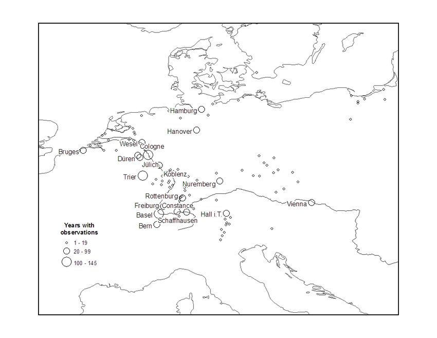
The following map shows the spatial distribution of our exchange
rate observations. They are a sample of the transactions concluded on
the late medieval money market, whose composition is determined by the
survival and accessibility of the sources. The drawbacks of this are
obvious: Records in some cities are better preserved than in others, and
observations are concentrated in the western part of the area under
study, which as a whole is therefore imperfectly represented. However,
the resulting bias has one important advantage: Most observations are
found along the main artery of late medieval transcontinental trade, which
linked Northern Italy and the Netherlands. This implies that the
assumption of on-going trade, needed to carry out analyses based on the
Law of One Price, is not very demanding in our context.
9Figure 1: Exchange Rate Observations, 1350-1560: Spatial Distribution
Exchange rates were based on several types of transactions, three
of which are relevant here (cf. Spufford, 1986: l f., cf. table 1). First, there
was the most elementary one, manual exchange, i.e. the simultaneous
and on the spot exchange of coins of different currencies. Second, some
exchange rate notations appear in loans where the creditor agreed to
repay the sum he borrowed in a different currency. And finally, there was
the most sophisticated kind of exchange, which made use of bills of
exchange.
The Canonical ban on usury implies that lending money at interest
was illegal. Accordingly, rates mentioned in loans and bills of exchange
may have contained a hidden interest rate. For those found in bills, this
10applied if these were primarily used as credit instruments and not as a
means to transfer money between localities (in which case the exchange
rate probably contained a transport cost component, cf. de Roover, 1948:
62; Mueller, 1995; Munro, 2003: 543 ff.). Loans, at any rate, presumably
did conceal such an interest rate. Hence, there may have been a
systematic difference between these types of exchange rates and those
paid in manual exchange. Unfortunately, the sources specify the
underlying kind of contract in only about four percent of the cases – too
few to allow us to identify a systematic difference between exchange
rates based on bills and loans and those based on manual exchange.
In order to determine the actual share of such transactions in the
late medieval money market, we would need to know how many of those
rates where the sources do not record the type of underlying contract
were based on loans and bills, too. While there is no way to answer this
question precisely, we can assume that in most cases the authors of the
sources were not interested in recording if a transaction was based on
manual exchange, as this was the most simple and straightforward type
of exchange. Bills and loans, however, i.e. transactions over time and
possibly space, needed to be carefully noted. We can therefore assume
that the sources do explicitly mention such bills and loans as there were.
Moreover, we need to take regional variations into account. Bills were
often employed in some Western European markets such as Bruges, but
though they were known in Central and Northern Europe, merchants
rarely made use of them there (de Roover, 1948: 55, 60; Spufford, 1991:
254 ff.). Out of the c. 600 observations from merchant account books and
areas outside England and Flanders that we have, only 1 refers to a bill of
exchange (from Cologne to Bruges: Lesnikov, 1973: 13). Even in
Flanders, non-cash means of payment made a negligible contribution to
monetary circulation overall (Blockmans, 1990: 26; cf. Murray, 2005:
123).
11The question of how the fine gold and silver content of the coinage
developed involves difficulties of its own. Apart from the fact that late
medieval sources are often ambiguous because their authors did not
clearly identify the coins they were exchanging, there are four issues that
need to be highlighted. First, the documents containing information on the
bullion content of the late medieval coinage, that is primarily ordinances
and contract between political authorities and the mint personnel, are
difficult to interpret. On the one hand, in some cases one cannot be
certain about the exact metric equivalents of the many local or regional
units of weight used in the mints. On the other hand, the ability of
medieval and early modern mint technicians to make chemically pure
gold and silver has been questioned (Miskimin, 1963: 31; Jesse, 1928:
160). This latter problem is important because in some cases it is not
clear whether the documents talk of 100 percent pure precious metals
that were to be alloyed with specified quantities of base metals such as
copper, or if what they mean is gold and silver of the highest purity that
could be manufactured (e.g. ‘argent le roi’ of 95.7 percent purity), to which
the copper was to be added (cf. van der Wee and Aerts, 1979: 61 f.;
1980: 234 ff.). We assume here that, if not explicitly stated otherwise, the
sources presupposed argent le roi and gold of corresponding purity as
raw materials.
A second difficulty is posed by the fact that usually – the Pound
Sterling being the most important exception – the bullion content of
different denominations belonging to the same currency was not
proportional: Small denominations contained proportionally less silver
than larger ones (de Roover, 1948: 222). Here, we assume that most
people did not pay for high-purchasing-power gold coins with small
change, but used the largest silver denominations available.
Debasements and re-enforcements pose a third difficulty because
there is no first-hand information on how long it took to replace old coins
12in circulation with new ones. This depended on several circumstances,
most importantly on whether the bullion content was reduced or
increased. If, in the first case, the nominal value of the monetary units
remained the same, it was in everybody’s interest to exchange old coins
for new ones as quickly as possible. In contrast, if the coinage was re-
enforced, we can, in line with Gresham’s Law, assume that old coins
tended to stay in circulation for longer. The distance to the mint is also
relevant: the larger it was, the longer would it take for new coins to
replace the old ones. This, finally, also depended on the mint output in the
period after the change in the standard. As with few exceptions – notably
England and Flanders – relevant data are almost entirely lacking. As we
work with yearly means, which obscure potential adjustments that took
place within weeks or months after changes in the monetary standards,
we focus on the distance to the mint, which we take into account after
monetary reforms (cf. Volckart and Wolf, 2006). Specifically, we assume
that within the home territory, new money replaced old coins within one
year, whereas abroad, adjustment entailed a time lag of one year.
A final difficulty is caused by the fact that, once in circulation,
money became worn down. For silver, losses due to wear and tear have
been variously estimated at between 2 and 2.75 percent per decade
(Mayhew, 1974: 3) and between 0.25 and 0.87 percent per year (North,
1990: 108; cf. Patterson, 1972). The higher purchasing power of gold
suggests that its velocity of circulation was lower than that of silver, so
that gold coins may have been exposed to less wear and tear.
Nonetheless we assume that coins made of both metals suffered alike
from defacement, so that its effects on gold and silver cancelled each
other out. This assumption is realistic, as silver was more often alloyed to
a higher degree with base metals; a process that increased its hardness.
To be sure, given that mint outputs varied, the average age of coins in
circulation must have varied, too. In this respect, our assumption that all
13coins were equally defaced is therefore unrealistic, but as in most cases
data on the output of mints do not exist, it is an acceptable simplification.
To reduce the noise caused by these factors, we rely on the results
of chemical tests conducted on the coins either by late medieval
authorities or by modern researchers (cf. e.g. Munro, 1972: 212 ff.;
Grierson, 1981; Kubiak, 1986). This helps us to determine how much gold
and silver changed hands when money was exchanged. In order to use
these data for the calculation of local gold-silver ratios, we finally need to
take into account the fact that on the market some gold currencies were
more popular than others. In consequence, gold-silver ratios that are
determined for one place, but on the basis of different types of coins are
not necessarily alike. As the great majority of transactions involve the
Rhinegulden, we examine only rates based on this coin. In addition, we
included only rates based on the most popular silver currencies used in
each locality.
3. Kondratieffs of Integration
The most common way of examining trends in market integration is
to consider the coefficient of variation, which is a dimension-less measure
equal to the standard deviation divided by the mean (Jörberg, 1972;
Toniolo et al., 2003; Jacks, 2004; Dobado González and Marrero, 2005;
Federico, 2007; Özmucur and Pamuk, 2007; Rönnbäck, 2009; Mitchener
and Ohnuki, 2009). The smaller it is, the lower is the level of ‘price’
dispersion and the greater that of market integration. As well as
examining the coefficient’s linear trend we use the augmented Dickey
Fuller test, which signals the presence of a permanent trend, to determine
whether there is evidence of a unit root (Özmucur and Pamuk, 2007;
Klovland, 2005). In addition, like Federico (2007) and Federico and
Persson (2007), we estimate the trend through the Epanechnikov kernel.
14This non-parametric technique permits the investigation of non-linear
behaviour. For the same reason, we estimate the trend also through
panel data analysis of the spreads (cf. Bateman, 2007).
As our data covers the years between 1400 and 1520
comparatively well, the yearly samples are based on relatively
homogeneous sets of cities. 2 There is only one year with fewer than four
observations, the yearly average being almost ten. While in the first half
of the sample there are on average fewer yearly means than in the
second, the difference is small: 8.85 as compared to 10.58. Low
seasonality means that the observations show hardly any variability within
years, so that the bias ensuing from examining annually-grouped data
from each city is limited. If anything, this bias should understate the
degree to which markets integrated, as the yearly averages are based on
more observations in the earlier part of the fifteenth century than in the
later period.
We test the robustness of the results against four sub-samples.
The first one is restricted to those cities for which at least 20 yearly
observations are available. This restriction entails a loss in terms of
representativeness, but offers gains in terms of homogeneity. The second
sub-sample consists of the three cities for which we have more than 100
yearly observations and of those years for which we have observations
from all of these cities. In this case, the cities covered do not vary from
year to year, but only some years are represented. In the third sub-
sample we exclude these cities in order to examine whether results are
influenced by their over-representation in the other samples. Finally, our
fourth sub-sample excludes all cities on the river Elbe or east of it, since it
is often assumed that due to late medieval trade patterns, financial
2
As differences in the sample composition across periods may affect patterns, a
homogenous panel of data is desirable to carry out this analysis. Still, analyses of the
coefficient of variations based on unbalanced panels are known in the literature
(Jörberg, 1972).
15markets exhibited persistent differences between gold-silver ratios in the
west and east (Watson, 1967; Flynn and Giraldez, 1995). This could
distort our results. 3
3
We owe this point to Sevket Pamuk. Interestingly, however, even if the analysis
presented in section 4 supports the claim that there were limited exchanges between
Western and Eastern Europe, our data gave rise to little or no evidence of systematic
variations of the gold-silver ratios between the two areas. The average gold-silver
ratios varied very little: 11.81 in the cities located at West of the Elbe, as compared to
11.85 in the others.
16Figure 2: Financial Integration in Central Europe: Coefficient of Variation
of the Gold-Silver Ratio, 1400-1520
all 20+
0.40 0.40
0.35 0.35
0.30 0.30
0.25 0.25
0.20 0.20
0.15 0.15
0.10 0.10
0.05 0.05
0.00 0.00
1390
1400
1410
1420
1430
1440
1450
1460
1470
1480
1490
1500
1510
1520
1530
1390
1400
1410
1420
1430
1440
1450
1460
1470
1480
1490
1500
1510
1520
1530
W100+ West
0.40 0.40
0.35 0.35
0.30 0.30
0.25 0.25
0.20 0.20
0.15 0.15
0.10 0.10
0.05 0.05
0.00 0.00
1390
1400
1410
1420
1430
1440
1450
1460
1470
1480
1490
1500
1510
1520
1530
1390
1400
1410
1420
1430
1440
1450
1460
1470
1480
1490
1500
1510
1520
1530
panel Financial integration and debasement
0.40 50
1.20 40
0.35
30
1.00 0.30
20
0.25 10
0.80 0.20 0
0.15 -10
0.60 -20
0.10
-30
0.40 0.05 -40
0.00 -50
0.20
1390
1400
1410
1420
1430
1440
1450
1460
1470
1480
1490
1500
1510
1520
1530
0.00
Debasement Poly. (Debasement)
1390
1400
1410
1420
1430
1440
1450
1460
1470
1480
1490
1500
1510
1520
1530
Poly. (all)
17Table 2: Financial Integration in Central Europe: Yearly Rates of Change
of the Coefficient of Variation of the Gold-Silver Ratio, 1400-1520 (in
percent)
Unit root
Sample Years N Rate test
1400- 10 per
All 1520 121 -0.087*** cent
1400- Not
20+ 1520 121 -0.070*** rejected
1404-
100+ 1520 84 -0.093***
1400- Not
W 100+ 1520 120 -0.102*** rejected
1400- 10 per
West 1520 121 -0.084*** cent
Key: N=sample size; 20+, 100+, W 100+, West=see text; ***=significant at the 1
percent level
The data show that overall the fifteenth century was a period of
financial convergence for Central Europe (fig. 2). By 1520, gold-silver
ratios tended to be considerably more uniform across cities than in 1400.
The robustness checks corroborate this result (table 2). In all samples –
even in the third, which is comparatively small – the yearly rate of change
of the coefficient of variation is negative and significant at the 1 percent
level. The speed of convergence is also estimated to be in the same
order of magnitude, 4 regardless of the sample. Moreover, in no case the
augmented Dickey Fuller test is able to reject non-stationarity at low
levels of significance, thereby providing support to the presence of a
trend. 5 In sum, there is strong evidence that the variability of the gold-
silver ratio tended to decrease over time.
4
The magnitude of the coefficient of variation is in the same order as that found by
Federico (2007) in the nineteenth-century Italian grain market, and considerably higher
order than that found in financial markets in the same place by Toniolo et al. (2003).
The comparison, however, can only be taken so far. Even if it is dimension-less, the
coefficient’s value does depend on the unit of measure. It is sufficient, for example, to
take the logarithm to obtain rather different results.
5
In the case of the ‘W 100+’ sample, one figure was interpolated.
18The rejection of the hypothesis of a unit root at the 10 percent level
in two instances can be traced to the fact that convergence, as the kernel
shows, was a discontinuous process. Again, the robustness checks
support the findings of the basic analysis. Almost identical cyclical
patterns emerge when using the unbroken sub-samples. The trend
detected by the random effects panel data analysis of the absolute value
of the gold-silver ratio difference is based on a comparison of the time
dummies coefficients with that of the first decade. Therefore, the initial
pattern differs. However, in subsequent years a similar pattern emerges.
The graphs signal a basic asymmetry between the 1410-1465 cycle
and the 1465-1520 one: In the second phase, long-term integration
advanced significantly more rapidly than during the earlier cycle. This
asymmetry fits both Munro’s (2001: 25) claim that the revival of late
medieval trade began in the early fifteenth century, and the widely held
view that trade experienced an upswing in the 1460s. The graphs also
clearly indicate cycles of integration about half a century long, i.e.
Kondratieff cycles (Kondratieff and Stolper, 1935). A number of scholars
(van der Wee, 1963; Abel, 1980; Tits-Dieuaide, 1975) have found waves
of similar duration in late medieval grain markets. The peaks of Abel’s
(1980: 64 f.) cycles of agricultural yields and prices in Central Europe
(1430s/1440s, late 1480s/90s) closely correspond to those of our waves
of integration, pointing to possible connections between agricultural and
financial dynamics.
The timing of the cycles of financial integration suggests that the
late medieval ‘bullion famines’ (e.g. Day, 1980/87; Day, 1981/87;
Spufford, 1991) are insufficient to explain them. One might argue that
under a commodity money system, where a scarcity of gold and silver
implied monetary contraction, a lack of coins should have increased
transaction costs and restricted opportunities for arbitrage in the money
market. It therefore should have had a direct impact on the dynamics of
19financial convergence. Yet, although particularly rapid convergence in the
early part of the fifteenth century did coincide with the end of a period of
bullion scarcity, there was no divergence during the mid-fifteenth century
bullion famine. On the contrary, between the 1440s and the 1460s local
gold-silver ratios markedly converged. There is, however, a strikingly
close correspondence between cycles of convergence and cycles of
debasement. 6 In the late Middle Ages as in modern times (van Duijn,
1977: 548 f.), Kondratieff cycles were associated with changes in the
money supply. 7
4. Uneven Integration
How far does this tendency towards financial integration apply to all
Central Europe? To answer this question, we examine financial
integration between pairs of cities basing ourselves on the following
measures: (1) the yearly rates of change of the absolute value of the
percentage gold-silver ratio difference; (2) the correlation rates of the
gold-silver ratios; and (3) the five years rolling coefficients of variation. 8
Yearly rates of change of the absolute value of the percentage gold-silver
ratio difference indicate whether and to what extent a locality was
integrating with others. A negative sign signals integration, a positive
disintegration. The higher the absolute value of the coefficient, the more
rapid the process was. The same interpretation applies to changes in the
coefficient of variation, where greater stability signals a less isolated
6
The cycles of debasement are based on the aggregate percentage reduction in the
bullion content of the most popular silver coins of the area: the Flemish Pound Grote,
the South-West German Pound Rappenmünze and the Pounds of Constance,
Württemberg and Nuremberg, the Albus of Cologne, the Penny of the Palatinate, the
Mark of Prussia, the Bohemian Groschen and the Kreuzer of Tirol.
7
Even if late medieval debasements are often treated as fiscal measures used in times
of war (Spufford, 1991; Munro, 2009), it needs to be kept in mind that debasing the
coinage was a means through which late medieval mints increased the money supply.
8
The last measure involves limited interpolation.
20market. Correlation rates, by contrast, provide a measure of the extent to
which gold-silver ratios developed stable linear relationships and thus of
how well two localities were integrated, with higher values signalling
greater levels of integration. 9 By combining the analysis of overall levels
and dynamics of integration, it is possible to gauge if integration improved
among weakly integrated markets.
To make a good use of the available data, we include observations
from before 1400 and after 1520. We limit the bias ensuing from working
with broken series by examining only those cities for which at least thirty
yearly observations are available. Specifically, the focus is on the seven
best-represented cities: Basel, Cologne, Düren, Hamburg, Koblenz, Jülich
and Trier. 10 In this way, we construct series whose size varies from a
minimum of 14 observations in the case of the pair Hamburg-Rottenburg
between 1396 and 1459, to a maximum of 124 for the pair Basel-Cologne
between 1396 and 1535. The average sample size is 52. Most of the
cities in the sample are in the Rhineland, with Cologne, Düren, Koblenz
and Jülich being relatively close to each other. Düren, Koblenz and Jülich
were also much smaller than Basel, Cologne and Hamburg, and
somewhat smaller than Trier. 11 The sample allows us to explore patterns
of long- and short-distance integration between centres of varying size
within the Rhineland, as well as of integration between the Rhineland and
other parts of the Empire.
9
Spurious correlation can arise in the presence of similar inflationary movements
across cities (Studer, 2008). However, as the series are not unbroken, in our case it
was not possible to differentiate them. In any case, given that the gold-silver ratio was
remarkably stable in the fifteenth century (Watson, 1967), this does not constitute a
serious problem.
10
This sampling implies that the correlation matrix is not symmetric, and thus factor
analysis could not be applied to identify underlining structures.
11
In our sample, Cologne is by far the largest city with c. 40,000 inhabitants in 1400
and 45,000 in 1500. Hamburg’s population is assumed to have shrunk from c. 22,000
to 15,000 over the period. Basel stayed overall constant (with intermittent fluctuations)
at c. 10,000 inhabitants, while Trier’s population fell from this level to about 8,000.
Düren, Jülich and Koblenz where much smaller places with under 5,000 inhabitants
each (Bairoch et al., 1988).
21Table 3: Financial Integration Between Cities in Central Europe: Yearly
Rates of Change of the Absolute Value of the Percentage Gold-Silver
Ratio Difference, Average Correlation Rates and Five Years Rolling
Coefficient of Variation (in percent)
Basel Cologne Düren Hamburg Jülich Koblenz Trier
Basel -0.08*** -0.11*** 0.03* -0.12*** -0.03** 0.01
Cologne -0.11*** -0.04*** -0.04* -0.02* -0.09*** -0.14***
Constance 0.10* -0.16*** -0.26 0.27** -0.18 -0.10** 0.05
Düren -0.13*** -0.04*** 0.07** -0.10*** 0.04 0.07
Freiburg -0.02 -0.03 -0.26 0.20*** -0.09* 0.06 0.02
Hall -0.28** -0.15 0.07 -0.06 0.40 -0.29** -0.03
Hamburg 0.04** -0.01 0.11*** 0.10** 0.07*** -0.02
Jülich -0.10*** -0.02* -0.08*** 0.09*** -0.05*** 0.08
Koblenz -0.04** -0.09*** 0.04*** 0.05** -0.06*** 0.06**
Nuremberg -0.07 -0.18 -0.63*** -0.10 -0.88*** -0.44** 0.04
Rottenburg 0.69*** -0.02 0.40** 0.38**
Trier 0.01 -0.09*** 0.12** 0.00 0.12** 0.08**
Vienna -0.11 -0.25*** -0.08*** -0.04 -0.25*** -0.24*** -0.01
Wesel -0.16* 0.01 1.00 0.07*** 1.10*** 0.75*** -0.27***
Average -0.01 -0.09 -0.01 0.07 0.00 -0.02 0.02
Correlation 0.23 0.31 0.38 0.06 0.24 0.33 0.20
Stability -0.03*** -0.04*** 0.02* 0.04** 0.03*** 0.00
Key: *=significant at the 10 per cent level, **=significant at the 5 per cent level, ***=significant at the 1
per cent level
The first fourteen rows of table 3 show the yearly rates of change of
the absolute value of the percentage gold-silver ratio difference. The last
three rows show the averages of the same figure, the averages of the
correlation rates, and the yearly rates of change of the coefficient of
variation. According to our results the process of financial integration was
uneven but widespread. In 52 out of 88 cases the absolute value of the
percentage difference of the gold-silver ratios tended to decline over time.
However, whereas in Basel, Cologne, Düren and Koblenz the average
yearly rate of change was negative, this was not the case in Hamburg,
Jülich and Trier. A tendency towards financial integration with the area is
22particularly marked in Basel and especially in Cologne. The sign of the
yearly rate of change of the absolute percentage gold-silver ratio
difference is negative in 9 cases out of 13 in Basel and in 12 out of 13 in
Cologne, as compared to, for example, 8 out of 12 cases in Jülich and 4
out of 13 in Hamburg. Even more clearly, the gold-silver ratios tended to
become more stable only in Basel and Cologne. The small centres
tended to be relatively well-integrated, but the evidence of progress is not
as strong. At the negative end of the spectrum, Hamburg shows very
weak integration and hardly any increase.
Table 4: Financial Integration Between Cities in Central Europe: Average
Correlation Rates and Yearly Rates of Change of the Absolute Gold-
Silver Ratio Difference (in percent) by Distance (in kilometres)
Distance Corr Trend N
600 9.5 -0.5 11
Key: Corr=correlation rate, N=sample size.
These observations conform to a wider pattern: Whereas, as
expected, the average correlation rate declines monotonically with
distance, the average yearly rate of change of the absolute gold-silver
ratio difference does not (table 4). Specifically, the figures evidence two
parallel processes of integration: One at the local level, between well-
integrated cities; and another somewhat stronger of long-distance
integration between weakly-integrated localities. Medium and very distant
cities did not tend to integrate.
Late medieval land transport was quicker than water transport, but
also more expensive and inconvenient for moving bulky loads (Bernard,
1972: 285). Conversely, it was well-suited to small-scale, quick and short-
23distance arbitrage. Still, potential improvements in land transport do not
explain why the process broke off beyond the very local level. Given the
Empire’s political fragmentation, the pattern might be consistent with a
role for intra-state integration (cf. Epstein, 1994: 475; 2000: 147 ff.).
However, inspection of the sample reveals that none of the city-pairs in
the group of very close cities experiencing integration – Basel-Freiburg,
Cologne-Düren, Cologne-Jülich and Düren-Jülich – were ruled by the
same lord. Indeed, Cologne was autonomous. All these pairs, on the
other hand, were linked by an either official or de facto monetary union.
By contrast, all city-pairs in the group of cities which were at a
comparable distance (70 - 150 kilometres instead of < 70 kilometres), but
which on the whole did not experience integration, were not part of the
same monetary union. Thus, it seems that monetary unions tended to
develop between well-integrated financial markets and favoured further
financial integration (Boerner and Volckart, 2008).
The correlation rates indicate that Basel was integrated
comparatively well with most of the cities in South Germany (Constance,
Freiburg, Hall, Nuremberg and Rottenburg), but there is strong evidence
of advances in integration only in the case of Hall in Tirol, in whose
neighbourhood large deposits of silver ore were discovered in the 1460s,
and where most South German mints purchased their bullion (Bissegger,
1917; Schüttenhelm, 1984; Palme, 1984). Hence the rise of South
German cities in the wake of the mining boom of the 1460s seems to
have had a limited direct effect on the dynamics of financial integration.
The rise of these cities, however, may have had also an indirect
impact, as it led to the development of an important trade route along the
Rhine that connected the region with Flanders and Brabant (Cipolla,
2002: 323; Spufford, 2002b: 391 f.). Comparatively strong evidence of
financial integration between Basel and Cologne, by far the largest city in
the sample, suggests that long-distance financial integration may have
24been linked to the growth of inter-regional financial centres in the
Rhineland. 12 In this area the concentration of financial services began
later than in Italy and the Flanders and involved, among other things, the
emergence of Basel as an important source of credit for neighbouring
rulers (Meyer, 2000: 46; Scott and Scribner, 1997). Qualitative evidence
also points to Cologne’s importance as a centre of the bullion trade and to
links to cities further south, in particular to Frankfurt and Basel (Irsigler,
1971: 371 f.). The process could have contributed to integration also in
Trier, but a declining population suggests that the city failed to benefit
from its situation on the Mosel, a major tributary of the Rhine. Indeed, the
older view that Trier was a commercial centre of supra-regional
importance has been revised by recent research (Clemens and Matheus,
1996: 503, 523 f.). Trier was also characterised by the relatively late
establishment of a university (1473) and a printing industry with a
comparatively low output (1481). In these respects, it differs from Basel
and Cologne, where universities were founded in 1459 and 1396, and
where considerably more productive printing presses were established in
1466 and 1469. Hence, declining information costs may have played a
role in explaining the difference.
In the same way as land transport is expected to affect mainly
short-distance financial integration, long-distance financial integration
among previously weakly integrated places in the Rhineland is consistent
with an explanatory role of river transport and shipping technology. We
mentioned in the introduction how, according to Unger (1980), shipping
technology had a key role in promoting fifteenth-century long-distance
market integration. Melis (1967) also detects a widening in the scope of
fifteenth-century waterborne trade in the wake of changes in the cost
structure. In Central Europe, river traffic specifically was facilitated by the
12
This contrasts with Scott’s (1987) assessment on the economic decline of big Central
European cities in the fifteenth century amidst competition from the country-side.
25widespread creation of towpaths in the late Middle Ages (cf. Ellmers,
2007: 175) – a development that fits asymmetric patterns of convergence:
While per unit costs of water transport were always lower than those of
land transport, shipping goods upriver, where barges needed to be stoked
or towed, was still more expensive than downriver transport (Ellmers,
2007: 166). Thus, the flow of the Rhine explains asymmetries in long-
distance financial integration in almost all cases where this yardstick can
be applied: Basel integrated more rapidly with Cologne than Cologne with
Basel, and the same applies to Basel and Düren, Basel and Koblenz,
and, on the Mosel-Rhine route, to Trier and Cologne. Likewise,
disintegration was less rapid between Trier and Düren, Koblenz and
Jülich than between Düren, Jülich 13 and Koblenz and Trier.
The absence of financial integration between cities further apart
than 600 kilometres reflects the lack of integration between the Rhineland
and Eastern Europe: city-pairs that cover this divide always include
Hamburg and Vienna. Direct trade between the upper and middle
Rhineland, where the observations are concentrated, and those parts of
the East from where we have data does not seem to have been very
important. Thus, for instance, Hamburg participated less in inland trade
than in commerce between the North Sea and the Baltic (Lüders, 1910).
Moreover, Hamburg was a leading member of the Hanseatic League,
whose importance peaked in the late fourteenth and began to decline in
the fifteenth century (Dollinger, 1981: 364 ff.). In short, both trade flows
and declining costs may have played a role in explaining uneven financial
integration in the Rhineland.
13
To be precise, Düren and Jülich were located on Roer, a tributary of the Maas. They
were, however, also close to the Rhine.
265. Adjustment and Costs
To gain a more precise impression of how far markets were
integrating, and to investigate if financial integration in the Rhineland was
mainly due to declining costs as opposed to an increasing volume of
exchange, we examine seven pairs of cities (Basel-Cologne, Cologne-
Düren, Cologne-Jülich, Cologne-Koblenz, Düren-Jülich, Düren-Koblenz
and Jülich-Koblenz) through a threshold autoregressive (TAR) analysis of
the spread. The main features of the TAR-model are as follows: The
difference between the gold-silver ratios of two cities follows a random
walk when it lies within the thresholds of inaction determined by transport
and transaction costs. If the difference falls outside these thresholds,
however, arbitrage implies that the spread tends to converge back
towards equilibrium in a non-linear manner, so that the adjustment
process is faster the further away from the threshold the spread lies. A
greater volume of exchange implies a higher speed of adjustment.
TAR analysis has been extensively employed in recent market
integration research. Still, scholars have criticised it for the underlying
assumption that trade conditions are stationary and for the neglect of the
impact of indirect arbitrage (a point of criticism that applies to most other
techniques, too, cf. Fackler and Goodwin, 2001; Trenkler and Wolf, 2005;
Coleman, 2007; Federico, 2007; Özmucur and Pamuk, 2007; Ejrnæs et
al., 2008). Others have raised the objections that the results of the
analysis are not reliable when institutions like national banks interfere with
the market (Esteves et al., forthcoming 2009), and that the reliability of
TAR estimates depends crucially on the assumption of ‘weakly efficient’
markets (i.e. markets where agents use all the information available,
which is exclusively embodied in prices). Otherwise, violations of the
commodity points may not result in adjustment or adjustment may occur
before the commodity points are reached (Federico, 2008).
27To address the first issue, we relax the assumption of stationarity
and allow the estimated thresholds and speed of adjustments to follow a
linear trend and to experience a structural break (cf. van Campenhout,
2007). We limit the positive bias provoked by indirect arbitrage by
focusing on cities connected by on-going trade (cf. Federico, 2007). Basel
and Cologne were major commercial centres linked by an established
and increasingly important trade-route. As mentioned earlier, Düren,
Jülich and Koblenz were relatively small, but located in the vicinity of
Cologne to whose hinterland they belonged (Eiden and Irsigler, 2000: 48).
It should be stressed, however, that our approach can only limit the bias
rather than eliminating it. As it is typically the case in TAR analyses we
make the mutually contradicting assumptions that the price movement in
locality A at time t is on the one hand explained by trade with locality B
when measuring market integration between A and B, and on the other
hand by trade with locality C when examining integration between A and
C. Since networks of trade are typically complex and uneven, the bias
does not need to be equal across pairs. Hence, inaccuracies are bound to
influence comparisons as well as estimated levels.
We will see in relation to debasements that the results can indeed
be distorted by the intervention of non-market actors. Still, the model is
flexible enough to take such factors into account. Specifically, we use
dummy variables to control for the effect of monetary debasements on
adjustment, and we allow costs to experience a structural break after a
significant episode of debasement in order to control for its effect on
stability. In fact, the gold-silver ratio series often do come closer to each
other after debasements as a result of level shifts analogous to those
provoked by a sudden fall in transaction costs. An explanation of this
dynamic is that rulers frequently resorted to debasements in order to drive
out ‘bad’ money, i.e. worn-out and defaced coins or foreign coins of
similar nominal but lower intrinsic value (Cipolla, 1963; 1983). The
28circulation of such coins was bound to increase uncertainty and therefore
transaction costs in the money market. Debasements also eased
conditions by stimulating minting and increasing the money supply, thus
reducing transaction costs. As for efficiency, we excluded strong
inefficiencies by testing for stationarity before estimating the model
through conditional least squares; violations of the assumption of weak
efficiency are likely to be relative. Hence, we expect them to introduce a
bias into our results rather than to invalidate them.
Table 5 summarises the results of the analysis. The simple
specification is a conventional BAND-TAR (Lo and Zivot, 2001) with
dummies to control for the contribution of debasements to the adjustment
process. The second specification allows the threshold and the speed of
adjustment to follow a linear trend. The last one includes both trends and
a downward shift of the threshold in connection with the most significant
episode of debasement. Alfa is the speed of adjustment; we expect it to
lie between -1 and 0, with -1 signalling perfect and 0 no integration. The
half-lives, which denote the time it takes to reduce a shock by a half, 14
are measured in months. Tau is the threshold. As its estimation was
carried out through grid search based on twenty-one quantiles of the
absolute value of the spread, we did not compute its significance level.
‘Tau change’ is the slope of the trend followed by the threshold. ‘Shift’ is
the downward shift experienced by the threshold as a result of
debasement.
14
Equal to twelve times the logarithm of one half divided by the logarithm of one plus
the speed of adjustment.
29Table 5: Threshold Autoregressive Analysis Results
Basel- Cologne- Cologne- Cologne- Düren- Düren- Jülich-
City-pair Cologne Düren Jülich Koblenz Jülich Koblenz Koblenz
Model/Years 1467-1532 1468-1551 1470-1551 1467-1547 1470-1551 1468-1547 1470-1547
Simple Alfa -0.27*** -0.91*** -0.87*** -0.79*** -0.15** -0.74** -0.19
Tau 0.24 0.36 0.41 0.24 0 0.05 0
Half-life 26 3 4 5 50 6 37
Trend Alfa 0 -0.31* -1.62*** -0.89** -1.50*** -0.23 -0.86** 0.88
Alfa T -0.21 -1.00** -0.73** -0.95*** -0.71*** -0.69*** -2.25
Tau 0 0.32 0.88 0.60 0.77 1.13 0.05 1.16
Tau T 0.09 0.28 0.06 0 0.22 0.05 0.33
Half-life 0 22 Weeks 4 Weeks 21 4 ∞
Half-life T 36 1 6 3 7 7 Weeks
Shift Alfa 0 -0.50** -1.37*** -1.04*** -1.22*** -1.22** -0.86** 0.25
Alfa T -0.32 -0.98*** -0.66** -0.71*** -0.53*** -0.69*** -1.80
Tau 0 0.50 0.75 0.53 0.52 1.06 0.05 0.83
Tau T 0.24 0.25 0.11 0.10 0 0.05 0.41
Tau
change 0.79 -0.59 -0.19 0.43 0 0 0.70
Half-life 0 12 Weeks Weeks Weeks Weeks 4 ∞
Half-life T 22 2 8 7 11 7 Weeks
Shift 0.51 0.15 0.34 0.59 1.06 0 0.86
Key: *=significant at the 10 per cent level, **=significant at the 5 per cent level, ***=significant at the 1 per cent level
30In the basic model, the order of magnitude of the speed of
adjustment is in line with that estimated by Volckart and Wolf (2006) for
financial markets between late medieval Flanders, Lübeck and Prussia,
and thus considerably higher than in late nineteenth-century financial
markets that adjusted in days (Canjels et al., 2004). However, when
allowing for trends, adjustments between close cities (which Volckart and
Wolf did not examine) could occur in a matter of weeks, as in nineteenth-
century grain markets (Federico and Persson, 2007), which confirms that
close places were well-integrated. For Düren-Jülich and Jülich-Koblenz
particularly high estimates of the threshold shift signal that the results are
heavily distorted by debasement. These pairs therefore constitute
exceptions under the simple specification; otherwise, as expected, the
estimates of the half-lives are considerably and consistently lower among
close cities than for Basel-Cologne. The absence of adjustment between
Jülich and Koblenz at the beginning of the period corresponds to what
van Campenhout (2007) found in the contemporary Tanzanian maize
market. In our case, it reflects the fact that the 1510 debasement of the
Albus of Cologne introduced an unaccounted-for structural break that
triggered a significant increase in the volume of exchange. This is,
however, the only city-pair for which there is evidence of increased
exchanges over time. In the cases involving Cologne, declining speeds of
adjustment are partly produced by influential observations at the
beginning of the period.
Most of the estimates of the threshold are in line with those of
Volckart and Wolf (2006), who estimated the silver points to lie between
0.12 and 0.98, and of Kugler (2008), according to whom arbitrage in late
fourteenth century Basel began after a 7 percent threshold was crossed.
By comparison, our thresholds lie between 0 and 1.16. The latter is about
10 percent of the gold-silver ratio. This is in the order of ten times the
threshold Flandreau (1997) computes on the basis of direct estimation in
31You can also read