MTA-KDD'19: A Dataset for Malware Traffic Detection - CEUR ...
←
→
Page content transcription
If your browser does not render page correctly, please read the page content below
MTA-KDD’19: A Dataset for Malware Traffic Detection∗
 Ivan Letteri1 , Giuseppe Della Penna1 , Luca Di Vita1 , and Maria Teresa Grifa1
    Dept. of Information Engineering, Computer Science and Mathematics, University of L’Aquila

                                                 Abstract
          In the present paper we describe a new, updated and refined dataset specifically tai-
      lored to train and evaluate machine learning based malware traffic analysis algorithms.
      To generate it, we started from the largest databases of network traffic captures available
      online, deriving a dataset with a set of widely-applicable features and then cleaning and
      preprocessing it to remove noise, handle missing data and keep its size as small as possi-
      ble. The resulting dataset is not biased by any specific application (although specifically
      addressed to machine learning algorithms), and the entire process can run automatically
      to keep it updated.

1     Introduction
In the recent years, the growing number of cyber attacks motivated an intense research in the
field of malware detection, and nowadays cyber security professionals can rely on increasingly
effective and efficient detection techniques which, however, need to be constantly updated.
Indeed, malware detection itself presents a number of inherent challenges, first of all the ability
of maintaining an up-to-date knowledge base containing distinctive features of all the current
classes of malware.
    Most of the research is currently focusing on the use of machine learning techniques for
malware detection. This approach presents a number of advantages, first of all its capability to
automatically identify the malware characteristics by observing a set of training samples, and
generalise these results to detect new variants without having actually seen them before.
    Since network-based malware, such as botnets, is currently one of the most common kind
of malware, in this paper we focus on malware traffic analysis, which tries to detect malware
by analysing its behaviour in terms of data sent and received through a network.
    However, the quality of such classifiers is largely determined by the quality of the underlying
training dataset, and having a high-quality dataset requires to collect real malware traffic
data, keep it updated, and make this data actually usable by a machine learning algorithm.
Unfortunately, publicly available malware traffic databases are few, and mostly outdated.
    In the present paper we describe a complete process that creates an updated malware traffic
dataset suitable to train and evaluate machine learning based malware traffic classifiers. To
this aim, we apply a Knowledge Discovery in Databases (KDD) process, starting from the
largest databases of network traffic captures available online, deriving a dataset with a set
of widely-applicable features and then cleaning and preprocessing it to remove noise, handle
missing data and keep its size as small as possible. The resulting dataset is not biased by any
specific application (although specifically addressed to machine learning algorithms), and the
entire process can run automatically to keep it updated.
    It is worth noting that this process requires the right use of a number of different data
manipulation techniques and algorithms such as profiling, imputation and scaling, which in
   ∗ Copyright c 2020 for this paper by its authors. Use permitted under Creative Commons License Attribution

4.0 International (CC BY 4.0).
MTA-KDD’19: A Dataset for Malware Traffic Detection Letteri, Della Penna, Di Vita and Grifa
turn require a good knowledge of many different machine learning, data analytics and statistics
issues to be effectively applied. As a part of our contribution, we try to make all these steps
completely transparent to the researchers who just want to develop and effectively test a new
malware traffic classifier.
We evaluate the dataset quality by measuring the presence of malware through anomaly
detection and present an experiment where the dataset is used to build a simple deep neural
network classifier which reaches a very high detection rate.
Of course, both the current dataset and its generation algorithm have been made available
to the research community.
2 Related work
Malware features extraction and selection is a largely addressed topic in the literature. As
an example, Cabau et al. [6] extract malware features by dynamically executing malware in
a controlled environment and monitoring three types of actions: filesystem writes, registry
operations and network access operations. arkac et al. [43] address the specific problem of
feature extraction for metamorphic malware, whereas Zhao et al. [42] focus on feature extraction
and selection from Android applications. Zhang et al. [40] perform feature selection for malware
detection introducing the novel Ensemble Feature Selection technique, which aims at reducing
the number and size of the selected features in order to obtain datasets easier to handle. Finally,
Arora et al. [3] also address the issue of android malware detection, but to this aim they use
features extracted from the network traffic generated by malware apps coming from the Android
Malware Genome Project, which makes this approach slightly more similar to our malware
traffic analysis context.
However, a common characteristic of all such kind of works is that they present feature
extraction and selection techniques and examples of features extracted using the proposed
methodologies, but never provide the researchers with a full, realistic dataset created through
their approach. Moreover, when a malware detection technique is also proposed, it is often
evaluated on a specifically-tailored dataset, making any comparison difficult.
The majority of the publicly-available malware detection datasets, like Android PRAGuard
[23], the Android Malware Dataset [38] or EMBER [2] are devoted to malware detection in
executable files, in particular Android applications. Indeed, the current literature presents
few works concerning the creation of public datasets for malware traffic detection purposes.
Therefore, most papers presenting malware traffic analysis algorithms usually carry on their
experiments using some classical, although outdated, datasets like CTU13 [10], UGR’16 [21],
CCC09 [13] or KDD99 [37]. However, while these datasets can be a suitable benchmark to
compare different approaches, they cannot give realistic information about the quality of a
malware detector, since they do not take into consideration current malware and its novel
attack mechanisms.
3 The MTA-KDD’19 Dataset
The traffic data used to build our dataset was extracted from two distinct sources:
• legitimate traffic comes from pcap files marked as Normal in the Malware Capture
Facility Project (MCFP) belonging to the Stratosphere project. In particular, the traffic
collected so far from the MCFP project is composed of 15 pcap files with a total size
greater than 7 GByte.
2MTA-KDD’19: A Dataset for Malware Traffic Detection Letteri, Della Penna, Di Vita and Grifa
• malicious traffic comes from the MTA [9] repository, which offers a collection of over one
thousand four hundred zip files, each containing one or more pcap files. Every binary file
in these pcaps has been recognised as malicious by IDS and Antivirus softwares (Suricata
[26], VirusTotal [8]). It is worth noting that the pcap files provided by MTA are password
protected, so we developed an ad-hoc scraping algorithm that automates their download
and decompression. The currently collected MTA traffic is made up of 2112 pcap files,
with a total size of than 4.8 GB. These observations cover a time span from June 2013 to
August 2019.
The MTA repository receives almost daily new traffic logs. Our framework performs peri-
odic downloads of these data, so our dataset is constantly growing and is constantly updated.
However, since the frequency of malware traffic updates is much higher than the legitimate one
(from MCFP), balancing the two parts is not trivial.
3.1 Dataset Features
The typical approach to build detection models is to run a bot in a controlled environment
and monitor its outgoing network connections. Unfortunately, this process is not as easy as it
seems: for example, bots often open a large number of additional connections to legitimate sites
to create some “noise” so, to identify the real command and control (C&C), it is necessary to
observe all the network traffic produced by a bot in a long period of time. The traffic features
to be observed must take in account this issue, and try to ”summarise” the bot behaviour
throughout time with a set of meaningful measures.
Moreover, since network connections (especially for malicious traffic) are nowadays always
encrypted, it is not possible to analyse the packet payload. Therefore, features must be extracted
from observable characteristics of the traffic like the packet ratio, length or protocol. Such
characteristics are typically aggregated in time windows to extract statistical measures that
actually represent the features. In this approach, the packets present in each pcap file are split
in subsets spanning a fixed amount of time (e.g., 15 minutes as used in [19]). However, time-
based aggregation requires an arbitrary choice, i.e., the window size, which may have a great
impact in the dataset quality, since different attack types often require different windows sizes
to be captured. Moreover, since pcap files are varying in size, time-based aggregation always
leads to discarding a certain amount of information at the end of each pcap. Therefore, in our
approach, we adopted a different strategy, by aggregating packets in each pcap having the same
source address (i.e., coming from the same host) in segments, even if they are not sequential in
time. This allows us to have a different point of view on the traffic, that takes into account the
hosts involved in the traffic rather than the packet flow itself. Moreover, common attacks such
as DDoS are much more easily identified if features like the packet ratio are calculated relative
to the hosts, and not to the overall traffic: indeed, in the latter case, the overall background
traffic, interleaving the attack packets, may make the attack less evident.
We extracted a total of 50 features, which are reported in Table 2 together with their
formulas. Note that, for sake of simplicity, unless otherwise specified from now on with packets
we refer to the packets present in a specific segment, i.e., packets in a particular pcap file
having all the same source address. Moreover, we summarise in Table 1 some meaningful sets
and functions that will be used to simplify the feature formulas.
These selected features have been inspired by several best practices in the field of malware
detection, as well as by the observation of the current malwares. The relevance of each feature
is briefly discussed in the following. In particular, each feature in the table has an associated
relevance note in the ”rel” column.
3MTA-KDD’19: A Dataset for Malware Traffic Detection Letteri, Della Penna, Di Vita and Grifa
S = {p0 , . . . , pn } the sent packets
S DN S sent packets using the DNS protocol
S T CP sent packets using the TCP protocol
S U DP sent packets using the UDP protocol
SH sent packets using the HTTP protocol
S HR sent packets containing an HTTP request
S DQ sent packets containing a DNS question record
S DR sent packets containing a DNS resource record
S ACK sent TCP packets with the ACK flag set
S SY N sent TCP packets with the SYN flag set
S F IN sent TCP packets with the FIN flag set
S P SH sent TCP packets with the PSH flag set
S U RG sent TCP packets with the URG flag set
S RST sent TCP packets with the RST flag set
S ACKSY N sent TCP packets ith both the ACK and SYN flags set
S small sent packets with payload length < 32 (small packets)
Dp distinct packet destination ports
Da distinct packet destination addresses
U distinct user agents in the HTTP sent packets
R the received packets
dom(p) number of domains referred in DNS packet p
len(p) payload length of packet p
nchar(s) number of characters in s
ndot(s) number of dots in s
nhyph(s) number of hyphens in s
ndigit(s) number of digits in s
ndnsque(p) number of items in question section of DNS packet p
ndnsans(p) number of items in answer section of DNS packet p
ndnsadd(p) number of items in additional section of DNS packet p
ndnsaut(p) number of items in authority section of DNS packet p
occur(s) number occurrences of each distinct value in the set s
t(p) arrival time of packet p
ttl(p) TTL reported in DNS packet p
valid(s) true if all the domain names th set s are valid
Table 1: Functions and sets used in the feature definition formulas.
1. Features {Ack,Syn,Fin,Psh,Urg,Rst}FlagDist: have been chosen since it has been empir-
ically shown (see, e.g., [1], [17], [39]) that the presence many packets with of certain TCP
flags set may indicate malware traffic.
2. Features {TCP,UDP,DNS}OverIP: have been chosen since many attacks exploit specific
characteristics of these protocols. As an example, trojans and other remote access issue
a large number of DNS requests to locate their command and control server, so an high
DNSOverIP ratio may indicate malicious traffic [25].
3. Features MaxLen, MinLen, AvgLen, StdDevLen, MaxIAT, MinIAT, AvgIAT, AvgDelta-
Time, MaxLenRx, MinLenRx, AvgLenRx, StdDevLenRx, MaxIATRx, MinIATRx, Av-
gIATRx,StartFlow, EndFlow, DeltaTime, FlowLen, FlowLenRx: have been chosen since
packet number, size and inter-arrival times are useful to detect flooding-style attacks
[16, 17].
4. Feature PktIORatio: has been chosen since in DDoS-style attacks the number of sent
packets is much higher than the received ones [36].
5. Feature FirstPktLen: has been chosen since many times the first sent packet reveals useful
characteristics of the traffic (see, e.g., [14], [28]).
4MTA-KDD’19: A Dataset for Malware Traffic Detection Letteri, Della Penna, Di Vita and Grifa
feature formula notes rel rem
|S T CP |
f FlagDist |S|
· |S f | with f ∈ (1) -
{Ack, Syn, F in, P sh, Rst}. un-
available if not TCP
|S p |
pOverIP |S|
with p ∈ {T CP, U DP, DN S} (2) -
t(pn )−t(p0 )
AvgDeltaTime |S|
zero if |S| = 1 (3) (1)
P
u∈U nchar(u)
AvgDistinctUALen PDistinctU A
NaN if |S HR | = 0 (12) (3)
nchar(dom(pj ))
pj ∈S DQ
AvgDomainChar P
|dom(pj )|
NaN if |S DQ | = 0 (8) (3)
pj ∈S DQ
P
ndigit(dom(pj ))
pj ∈S DQ
AvgDomainDigit P
|dom(pj )|
NaN if |S DQ | = 0 (8) (3)
pj ∈S DQ
P
ndot(dom(pj ))
pj ∈S DQ
AvgDomainDot P
|dom(pj )|
NaN if |S DQ | = 0 (8) (3)
pj ∈S DQ
P
nhyph(dom(pj ))
pj ∈S DQ
AvgDomainHyph P
|dom(pj )|
NaN if |S DQ | = 0 (8) (3)
pj ∈S DQ
P
ttl(pj )
pj ∈S DR
AvgTTL - (9) (3)
|S DR |
DeltaTime t(pn ) − t(p0 ) zero if |S| = 1 (3) -
DistinctUA |U | - (12) (3)
|S DN S | P
DNSADist |S|
· p ∈S D ndnsans(pj ) - (6) (1)
j
|S DN S | P
DNSQDist |S|
· pj ∈S D ndnsque(pj ) - (6) -
|S DN S | P
DNSRDist |S|
· p ∈S D ndnsadd(pj ) - (6) (1)
j
|S DN S | P
DNSSDist |S|
· p ∈S D ndnsaut(pj ) - (6) (1)
j
EndFlow t(pn ) - (3) (1)
FirstPktLen len(p
P 0) - (5) -
FlowLen len(pj ) - (3) -
Ppj ∈S
FlowLenRx pj ∈R len(pj ) - (3) -
H
HTTPpkts |S | - (12) -
MaxIATRx, min of {(t(pj ) − t(pj−1 ))|pj ∈ R} zero if |R| < 2 (3) (1)
MinIAT, MaxIAT, Av- min, max, avg of {(t(pj ) − zero if |S| < 2 (3) -
gIAT t(pj−1 ))|pj ∈ S}
MinIATRx, AvgIATRx min, avg of {(t(pj ) − t(pj−1 ))|pj ∈ zero if |R| < 2 (3) -
R}
MinLen, MaxLen, Av- min, max, avg, stddev of StdDevLen is NaN if |S| < 2 (3) -
gLen, StdDevLen {len(pj )|pj ∈ S}
MinLenRx, MaxLenRx, min, max, avg, stddev of StdDevLenRx is NaN if |R| < 2 (3) -
AvgLenRx, StdDe- {len(pj )|pj ∈ R}
vLenRx
NumConnections |S ACKSY N | unavailable if not TCP (10) -
NumDstAddr |Da | - (11) -
NumPorts max{|Dp |} unavailable not TCP or UDP (11) -
|R|
PktIOratio |S|
- (4) -
max occur({len(pj )|pj ∈S})
RepeatedPktLenRatio |S|
- (7) -
|S small |
SmallPktRatio |S|
- (7) -
StartFlow t(p0 ) - (3) -
|S S |
SynAcksynRatio unavailable if not TCP, NaN if (10) (3)
|S ACKSY N |
|S ACKSY N | = 0
|S T CP |
UrgFlagDist · |S U RG | unavailable if not TCP (1) (2)
n |S| o
| pj ∈S DQ |valid(dom(pj )) | DQ
ValidURLratio DQ NaN if |S |=0 (8) (3)
|S |
Table 2: Dataset features.
6. Features DNSQDist,DNSADist,DNSRDist,DNSSDist: have been chosen since, as already
described, malwares often send DNS requests with specific characteristics [25].
7. Features RepeatedPktLenRatio, SmallPktRatio: has been chosen since in DDoS-style
5MTA-KDD’19: A Dataset for Malware Traffic Detection Letteri, Della Penna, Di Vita and Grifa
attacks it is often possible to observe a large number of (automatically generated) small
packets sent in sequence [14].
8. Features AvgDomainChar, AvgDomainDot, AvgDomainHyph, AvgDomainDigit, ValidUrl-
Ratio: have been chosen since often the domains involved in malicious traffic have names
with specific characteristics like unusual length or presence of dots and hyphen charac-
ters [24].
9. Feature AvgTTL: has been chosen since it is known that setting TTL values to very low
values can help the malware to change the C&C server rapidly or, on the other hand,
there are some advanced malware domains setting very high TTL values [41].
10. Features NumConnections, SynAcksynRatio: have been chosen since, in DDoS attacks,
the target is unable to satisfy all the connection requests, which become much higher
than the actually established connections (identified by the SynAcksynRatio: see, e.g.,
the DDoS attack principle as described in [7]).
11. Features NumDstAddr, NumPorts: has been chosen since, especially in DDoS-style at-
tacks, all the attackers are connected to the same victim, whereas the victim has open
connections with a large number of different hosts (the attackers) [22].
12. Features DistinctUA, AvgDistinctUALen, HTTPPkts: have been chosen since the user
agent field can be exploited to inject malicious code in the request, and of course HTTP
requests are the most common for malwares. Actually, almost one malware out of eight
uses a suspicious UA header in at least one HTTP request [11].
4 MTA-KDD’19 Generation Process
Figure 1: Overview of MTA KDD’19 generation process.
In this section we describe the automatic process that generates the MTA-KDD’19 dataset,
with the features listed in Section 3.1. The overall process is depicted in Figure 1.
6MTA-KDD’19: A Dataset for Malware Traffic Detection Letteri, Della Penna, Di Vita and Grifa
In particular, we try to apply a minimal preprocessing on the data, limited to the manip-
ulations needed to make the dataset suitable to be used in machine learning applications and
optimise its performances, e.g. by removing unnecessary data. Therefore, we are confident that
the resulting dataset is not biased by any particular application.
4.1 Feature extraction
As introduced in the previous section, to build the initial dataset, i.e., to extract the traffic
features, for each distinct pcap file, we group the contained packets based on the source address
(segmentation), and then compute the features in Table 2 on these groups. The set of features
related to a specific segment become a row of our dataset, that we shall call dataset sample.
Stating from the pcap files described in Section 3, we obtain a dataset with the characteristics
shown in Table 3. It is worth noting that the dataset is balanced, i.e., the distribution of malware
and legitimate samples is very similar.
Sample Type Sample Count Percentage
Malware 39544 55.3%
Legitimate 31926 44.7%
Total 71470 100%
Table 3: Composition of the MTA-KDD’19 dataset.
4.2 Profiling
In the profiling phase we analyse the dataset features in order to detect and remove certain
low-complexity issues that may affect the data and influence the next phases. In particular, we
perform the following steps.
Duplicates Duplicate samples may influence the classifiers and cause overfitting. Even if the
source dataset showed a very low number of duplicates, we remove them all.
Highly-correlated features During the profiling phase we also extract useful information
about the feature correlation, which is measured using the Pearson method [29]. Features with
a high correlation, ≥ 0.95 in our case, are removed from the dataset since they do not convey
additional information and, if preserved, would only increase the amount of resources needed
to process the dataset in the following phases. Therefore, we randomly select a feature in each
high-correlation pair and remove it. In particular, the removed features are AvgDeltaTime
(correlated to AvgIATRx with ρ = 0.96199), MaxIATRx (correlated to MaxIAT with ρ =
0.99853), DNSADist (correlated to DNSQDist with ρ = 0.99564), DNSRDist (correlated to
DNSADist with ρ = 0.97725), DNSSDist (correlated to DNSRDist with ρ = 0.9981), EndFlow
(correlated to StartFlow with ρ = 1). In table 2 the features removed for high correlation are
marked with the number (1) in the ”rem” column.
Zeros, Unavailable Values, and Missing Values Some features may have zero values for
different reasons. ”Real” zeroes are those that are useful to classify the traffic, but sometimes
a zero may be used to represent an unavailable value, which has a very different meaning, i.e.,
in some sense, it must be ignored by classifiers, since it does not convey any information (e.g.,
TCP-specific features are unavailable in UDP traffic). Finally, since traffic data tend to be
7MTA-KDD’19: A Dataset for Malware Traffic Detection Letteri, Della Penna, Di Vita and Grifa
algorithm GNB LogReg RF
standardized scaler 75.96% 90.64% 94.20%
minmax scaler 75.96% 85.93% 94.41%
maxabsolute scaler 75.96% 85.91% 94.41%
robust scaler 69.36% 48.21% 94.20%
quantile transformer 78.07% 91.97% 94.20%
power transformer 80.69% 97.31% 94.20%
Table 4: Weighted average precision metrics after scaling evaluated with three different classi-
fiers.
incomplete and noisy, as we already noticed in the formulas, some features may have missing
values indicated by a Not a Number (NaN) value.
Based in this, we first remove the URGFlagDist feature that is set to zero in all the samples,
so it seems to not convey any information about the traffic. In table 2 this feature is marked
with the number (2) in the ”rem” column.
Then, we remove any sample that contains an unavailable feature value. With this filter,
we drop 6828 samples, whereas the remaining dataset has still 64554 samples, 53.21% of which
represent malware and 46,79% legitimate traffic, so the dataset is now even more balanced.
Finally, features with many NaN (≥ 50%, so with a small number of real values), are removed
from the dataset since they do not convey enough information. In particular, the removed fea-
tures are AvgDomainChar (97.6% missing values), AvgDomainDot (97.6%), AvgDomainHyph
(97.6%), AvgDomainDigit (97.6%), AvgTTL (99.7%), SynAcksynRatio (96.5%), ValidURLra-
tio (97.6%), DistinctUA (96.6%), AvgDistinctUALen (96.6%). In table 2 the features removed
for high correlation are marked with the number (3) in the ”rem” column.
4.3 Imputation
In the previous phase we removed the features containing too much missing values. However,
all the remaining NaN (still present in the two features StdDevLen and StdDevLenRx) must be
replaced with real(istic) values in order to fed the dataset to a classifier. The imputation phase
compensates these missing values based on the other, concrete values of the same feature.
To this aim, we selected the Multivariate Imputation by Chained Equation (MICE) algo-
rithm, which has high performance and efficiency. This type of imputation works by filling the
missing data multiple times. Multiple imputations are better than a single imputation as they
measure the uncertainty of the missing values more precisely. The chained equations approach
is also very flexible and can handle different variables of different data types (i,e., continuous
or binary) as well as bounds or skip patterns [4].
4.4 Scaling
The dataset contains features highly varying in magnitudes, units and range. Since most
machine learning algorithms use the Eucledian distance between two data points in their com-
putations, it is necessary to scale the data with appropriate methodologies.
However, feature scaling may heavily influence the results of some algorithms. Therefore,
we first select three affine transformers and two nonlinear transformers i.e., MinMaxScaler
[31], MaxAbsScaler [30], StandardScaler [35], RobustScaler [34], QuantileTransformer [33] and
PowerTransformer [32], and try to scale the features with each of them. Then, to have a raw
idea of the impact of such scaling on a machine learning algorithm, we use 70% of the scaled
dataset to train three classifiers, namely Gaussian Naive Bayes (GNB), Random Forest (RF),
8MTA-KDD’19: A Dataset for Malware Traffic Detection Letteri, Della Penna, Di Vita and Grifa
and Logistic Regression (LogReg), and then evaluate the reached classifier quality by computing
its weighted average precision (i.e., the ratio between correctly predicted positive observations
and total predicted positive observations) on the remaining 30%. The results in Table 4 show
that the PowerTransformer makes two of the three classifiers reach the highest precision, so our
dataset generation process will adopt this scaling methodology.
5 Dataset Evaluation
Once the dataset is correctly setup, we can apply some further techniques to evaluate its quality
and suitability for machine learning algorithms. In particular, we first want to understand if
it actually contains an adequate amount of outliers, which can be seen as not-normal traffic
samples and can be detected by a ML classifier as anomalies, i.e., possible malware. Then, we
will also verify the detection accuracy that a more powerful (w.r.t. the GNB used for scaler
evaluation) classifier can reach using this dataset.
5.1 Outlier Detection
The basic assumptions for anomaly detection in network traffic are that “The majority of the
network connections are normal traffic, only a small percentage of traffic are malicious” [27]
and that “The attack traffic is statistically different from normal traffic” [15].
Given the size of our dataset, we cannot apply such an outlier detection to all the features
in all the samples. Therefore, we estimated the feature importance based on the Gini index
of each feature on the entire dataset through a random forest (RF) classifier [5], and selected
the six features with the highest score (the most informative ones), i.e., DNSQDist, StartFlow,
MinIATRx, MaxLen, DeltaTime and AvgIAT. Then, we selected the largest malware pcap from
Figure 2: Distribution of the six features with highest importance.
MTA (258.5 MB) and extracted the dataset samples corresponding to its packets. Finally, we
identified the outliers following the commonly-used rule that marks a data point as an outlier if
it is more than 1.5 · IQR above the third quartile or below the first quartile, where IQR is the
Inter Quartile Range. To this aim, we used the WEKA framework [12] on the selected features
of this reduced dataset.
9MTA-KDD’19: A Dataset for Malware Traffic Detection Letteri, Della Penna, Di Vita and Grifa
The results clearly indicate a large number of outliers, which are also graphically shown in
Figure 2 as red dots. To further check if such outliers can be actually associated to malware
traffic, we identified the IP addresses corresponding to the packets generating an outlier and
discovered that all these packets were marked as part of a malware attack in the source files.
5.2 Classification Experiment
The last quality measure for our final dataset is derived from a classification experiment realised
using a multilayer perceptron. In previous papers [20] we showed that this kind of classifier, if
correctly set-up and fed with a ”good” dataset, can reach a very high accuracy. However, the
dataset used in [20] was smaller and not updated with respect to the one we present here.
We used a multilayer perceptron with a quite trivial rectangle-shaped fully connected net-
work, trained for 10 epochs, with two hidden layers of 2f neurons each without dropout among
them, where f = 34 is the number of features in our final dataset. We performed a 5-cross
fold validation, by splitting the dataset in five segments and then performing five experiments,
each of which uses a different segment (thus 20% of the dataset) as test set and the rest (80%)
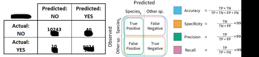
as the training set. In all the experiments the network performed in a very similar way: as
an example, Figure 3 shows the confusion matrix taken from one of the experiments, with an
accuracy of 99.74%. Actually, the average accuracy of all the experiments was 99.69% with a
standard deviation of 0.24%. Also the other metrics, i.e., specificity, precision and recall, have
very good values. This clearly shows that the dataset offers a good source of information to
detect current malware using a neural network classifier.
Figure 3: Confusion matrix and metrics of experiment #5.
6 Conclusions
In this paper we presented new dataset, namely MTA-KDD’19, built to ease testing and com-
parison of machine learning-based malware traffic analysis algorithms. The data sources used
are up-to-date, i.e. they contain the most recent malware traffic, and are continuously updated,
making the dataset quite realistic. Moreover, we performed an accurate feature selection and
data preprocessing in order to make the dataset as small as possible and effectively usable in
a ML classifier, without introducing any experiment or algorithm-specific bias. Indeed, some
preliminary quality measures on the final dataset show that it constitutes a good source of
information to train any kind of ML classifier. The complete dataset is publicly available [18],
and we will soon publish as open source on the same site the algorithm that can be used to
build and update it.
As a future work, we plan to apply more complex feature selection strategies in order to
further reduce the number of features to the most informative ones. Moreover, we are studying
10MTA-KDD’19: A Dataset for Malware Traffic Detection Letteri, Della Penna, Di Vita and Grifa
how to better handle unavailable feature values, in order to reduce the dataset samples excluded
due to this issues, and evaluating the impact of the imputation phase on the dataset quality. Of
course, we will further validate our dataset by evaluating its performances on different neural
network architectures and other machine learning models.
References
[1] Raihana Abdullah, Zaki Masud, Mohd Abdollah, Shahrin Sahib, and Y. Robiah. Recognizing
p2p botnets characteristic through tcp distinctive behaviour. International Journal of Computer
Science and Information Security, 9, 12 2011.
[2] Hyrum S. Anderson and Phil Roth. EMBER: an open dataset for training static PE malware
machine learning models. CoRR, abs/1804.04637, 2018.
[3] A. Arora, S. Garg, and S. K. Peddoju. Malware detection using network traffic analysis in android
based mobile devices. In 2014 Eighth International Conference on Next Generation Mobile Apps,
Services and Technologies, pages 66–71, Sep. 2014.
[4] Melissa J. Azur, Elizabeth Stuart, Constantine Frangakis, and Philip Leaf. Multiple imputation
by chained equations: What is it and how does it work? International Journal of Methods in
Psychiatric Research, 20(1):40–49, 3 2011.
[5] Leo Breiman. Random forests. Mach. Learn., 45(1):5–32, October 2001.
[6] G. Cabau, M. Buhu, and C. P. Oprisa. Malware classification based on dynamic behavior. In 2016
18th International Symposium on Symbolic and Numeric Algorithms for Scientific Computing
(SYNASC), pages 315–318, Sep. 2016.
[7] Z. Chao-yang. Dos attack analysis and study of new measures to prevent. In 2011 International
Conference on Intelligence Science and Information Engineering, pages 426–429. IEEE, Aug 2011.
[8] Chronicle Security. Virustotal. https://www.virustotal.com.
[9] Brad Duncan. Malware traffic analysis, 2019. https://www.malware-traffic-analysis.net.
[10] S. Garca, M. Grill, J. Stiborek, and A. Zunino. An empirical comparison of botnet detection
methods. Computers & Security, 45:100 – 123, 2014.
[11] Martin Grill and Martin Rehak. Malware detection using http user-agent discrepancy identifi-
cation. 2014 IEEE International Workshop on Information Forensics and Security, WIFS 2014,
pages 221–226, 04 2015.
[12] Mark Hall, Eibe Frank, Geoffrey Holmes, Bernhard Pfahringer, Peter Reutemann, and Ian H.
Witten. The WEKA data mining software: an update. SIGKDD Explorations, 11(1):10–18, 2009.
[13] Mitsuhiro Hatada, You Nakatsuru, Masato Terada, and Yoichi Shinoda. Dataset for anti-malware
research and research achievements shared at the workshop, 2009. http://www.iwsec.org/mws/
2009/paper/A1-1.pdf.
[14] Chien-Hau Hung and Hung-Min Sun. A botnet detection system based on machine-learning using
flow-based features. SECURWARE 2018 : The Twelfth International Conference on Emerging
Security Information, Systems and Technologies, 2018.
[15] H. Javits and Alfonso Valdes. The nides statistical component description of justification. Technical
report, Department of the Navy, Space and Naval Warfare Systems Command, 3 1994.
[16] Madhav Kale and D.M.Choudhari. Ddos attack detection based on an ensemble of neural classifier.
International Journal of Computer Science and Network Security, 14(7):122–129, 2014.
[17] G. Kirubavathi Venkatesh and R. Anitha Nadarajan. Http botnet detection using adaptive learn-
ing rate multilayer feed-forward neural network. In Ioannis Askoxylakis, Henrich C. Pöhls, and
Joachim Posegga, editors, Information Security Theory and Practice. Security, Privacy and Trust
in Computing Systems and Ambient Intelligent Ecosystems, pages 38–48, Berlin, Heidelberg, 2012.
Springer Berlin Heidelberg.
[18] Ivan Letteri. MTA-KDD’19 dataset, 2019. https://github.com/IvanLetteri/MTA-KDD-19.
11MTA-KDD’19: A Dataset for Malware Traffic Detection Letteri, Della Penna, Di Vita and Grifa
[19] Ivan Letteri, Giuseppe Della Penna, and Pasquale Caianiello. Feature selection strategies for HTTP
botnet traffic detection. In 2019 IEEE European Symposium on Security and Privacy Workshops,
EuroS&P Workshops 2019, Stockholm, Sweden, June 17-19, 2019, pages 202–210, 2019.
[20] Ivan Letteri, Giuseppe Della Penna, and Giovanni De Gasperis. Botnet detection in software
defined networks by deep learning techniques. In Springer International Publishing, editor, Pro-
ceedings of 10th International Symposium on Cyberspace Safety and Security, volume 11161 of
LNCS, pages 49–62, 10 2018.
[21] Gabriel Maci-Fernndez, Jos Camacho, Roberto Magn-Carrin, Pedro Garca-Teodoro, and Roberto
Thern. Ugr16: A new dataset for the evaluation of cyclostationarity-based network idss. Computers
& Security, 73:411 – 424, 2018.
[22] Tasnuva Mahjabin, Yang Xiao, Guang Sun, and Wangdong Jiang. A survey of distributed denial-
of-service attack, prevention, and mitigation techniques. International Journal of Distributed
Sensor Networks, 13(12):1–33, 2017.
[23] Davide Maiorca, Davide Ariu, Igino Corona, Marco Aresu, and Giorgio Giacinto. Stealth attacks:
An extended insight into the obfuscation effects on android malware. Computers And Security
(Elsevier), 51 (June):16–31, 2015.
[24] Khulood Al Messabi, Monther Aldwairi, Ayesha Al Yousif, Anoud Thoban, and Fatna Belqasmi.
Malware detection using dns records and domain name features. In Proceedings of the 2Nd Inter-
national Conference on Future Networks and Distributed Systems, ICFNDS ’18, pages 29:1–29:7,
New York, NY, USA, 2018. ACM.
[25] Asaf Nadler, Avi Aminov, and Asaf Shabtai. Detection of malicious and low throughput data
exfiltration over the dns protocol. Computers & Security, 80:36–53, 2017.
[26] Open Information Security Foundation. Suricata. https://suricata-ids.org/.
[27] Leonid Portnoy, Eleazar Eskin, and Sal Stolfo. Intrusion detection with unlabeled data using
clustering. In In Proceedings of ACM CSS Workshop on Data Mining Applied to Security (DMSA-
2001, pages 5–8, 2001.
[28] Paulo Angelo Alves Resende and Andr Costa Drummond. Http and contact-based features for
botnet detection. Wiley, 2018.
[29] Ronald Rousseau, Leo Egghe, and Raf Guns. Chapter 4 - statistics. In Ronald Rousseau, Leo
Egghe, and Raf Guns, editors, Becoming Metric-Wise, Chandos Information Professional Series,
pages 67 – 97. Chandos Publishing, 2018.
[30] Scikit-Learn. MaxAbsScaler. https://scikit-learn.org/stable/modules/generated/sklearn.
preprocessing.MaxAbsScaler.html.
[31] Scikit-Learn. MinMaxScaler. https://scikit-learn.org/stable/modules/generated/sklearn.
preprocessing.MinMaxScaler.html.
[32] Scikit-Learn. PowerTransformer. https://scikit-learn.org/stable/modules/generated/
sklearn.preprocessing.PowerTransformer.html.
[33] Scikit-Learn. QuantileTransformer. https://scikit-learn.org/stable/modules/generated/
sklearn.preprocessing.QuantileTransformer.html.
[34] Scikit-Learn. RobustScaler. https://scikit-learn.org/stable/modules/generated/sklearn.
preprocessing.RobustScaler.html.
[35] Scikit-Learn. StandardScaler. https://scikit-learn.org/stable/modules/generated/
sklearn.preprocessing.StandardScaler.html.
[36] Manoj Thakur, Divye Khilnani, Kushagra Gupta, Sandeep Jain, Vineet Agarwal, Suneeta Sane,
Sugata Sanyal, and Prabhakar Dhekne. Detection and prevention of botnets and malware in an
enterprise network. International Journal of Wireless and Mobile Computing, 5(2):144–153, 2012.
[37] The UCI KDD Archive. Kdd cup 1999 data, 1999. http://kdd.ics.uci.edu/databases/
kddcup99/kddcup99.html.
[38] Fengguo Wei, Yuping Li, Sankardas Roy, Xinming Ou, and Wu Zhou. Deep ground truth analysis
12MTA-KDD’19: A Dataset for Malware Traffic Detection Letteri, Della Penna, Di Vita and Grifa
of current android malware. In International Conference on Detection of Intrusions and Malware,
and Vulnerability Assessment (DIMVA’17), pages 252–276, Bonn, Germany, 2017. Springer.
[39] Y. Xiang, W. Zhou, and M. Guo. Flexible deterministic packet marking: An ip traceback system to
find the real source of attacks. IEEE Transactions on Parallel and Distributed Systems, 20(4):567–
580, April 2009.
[40] X. Zhang, S. Wang, L. Zhang, Chunjie Zhang, and Changsheng Li. Ensemble feature selection
with discriminative and representative properties for malware detection. In 2016 IEEE Conference
on Computer Communications Workshops (INFOCOM WKSHPS), pages 674–675, April 2016.
[41] G. Zhao, K. Xu, L. Xu, and B. Wu. Detecting apt malware infections based on malicious dns and
traffic analysis. IEEE Access, 3:1132–1142, 2015.
[42] K. Zhao, D. Zhang, X. Su, and W. Li. Fest: A feature extraction and selection tool for android
malware detection. In 2015 IEEE Symposium on Computers and Communication (ISCC), pages
714–720, July 2015.
[43] N. arkac and . Soukpnar. Frequency based metamorphic malware detection. In 2016 24th Signal
Processing and Communication Application Conference (SIU), pages 421–424, May 2016.
13You can also read