MYORIGINS 3.0 Combining Global and Local Methods for Determining Population Ancestry - FamilyTreeDNA Blog

MYORIGINS 3.0
Combining Global and Local Methods
for Determining Population Ancestry
 White Paper 2021-08-18

 Paul Maier • Rui Hu • Göran Runfeldt • Dunia Giniebra • Eric Frichot

2

Summary
FamilyTreeDNA team is excited to introduce MYORIGINS V3, our new tool for estimating
population ancestry. Population ancestry is the proportion of DNA you have inherited from each
ancestral population. Depending upon how much admixture occurred between your ancestors,
you may have inherited DNA from one or perhaps many populations.

We have updated many aspects of our pipeline, including:

 (1) An increase in number of reference populations from 24 to 90,
 (2) Improvements in precision and accuracy using our newest methodological advancements,
 (3) A chromosome painting:
 • You may learn the chromosomal location of each population segment,
 • This information may be genealogically valuable.

Contents
Glossary of Genetic and Analytical Terms __________________________________________ 3
Overview ____________________________________________________________________ 5
What is a Population? ________________________________________________________ 11
Reference Panel _____________________________________________________________ 13
 Data Sources _____________________________________________________________________ 13
 Finding Population Structure ________________________________________________________ 14
Overview of MYORIGINS v3 Pipeline _______________________________________________ 18
Global Ancestry – Speedymix ___________________________________________________ 20
Local Ancestry _______________________________________________________________ 21
 Phasing _________________________________________________________________________ 21
 Segment Classification _____________________________________________________________ 23
 Conditional Random Field __________________________________________________________ 25
 Phase Correction _________________________________________________________________ 27
Global-Local Ancestry Integration _______________________________________________ 29
Validation __________________________________________________________________ 31
Future Improvements _________________________________________________________ 41
References __________________________________________________________________ 42
Appendix ___________________________________________________________________ 46

FamilyTreeDNA – MYORIGINS 3.0

3

Glossary of Genetic and Analytical Terms
 Accuracy – Ability to classify something correctly.
 Admixture – Occurs when individuals of distinct population ancestries produce offspring, whose
 DNA is then a mosaic of ancestries (usually within a genealogical timeframe).
 Ancestry-informative marker – Marker with large allele frequency differences between populations;
 thus, they may be informative about a person’s population ancestry.
 Allele – One of two or more variants of DNA sequence found at a genetic locus (e.g., ‘T’).
 Autosomal – Describing all of the 22 pairs of chromosomes that exclude X, Y, and mitochondrion.
 Base pair (bp) – Smallest length of DNA; one complementary pair of DNA bases (nucleotides).
 Biallelic – A genetic marker (usually a SNP) possessing only two alleles in the population.
 Bifurcating tree – Phylogenetic tree where every divergence contains exactly two daughter branches.
 Centimorgan (cM) – A unit of distance along a chromosome. Between two chromosome positions
 that are spaced 100 cM apart, one recombination event is expected per generation.
 Chromosome – One unbroken strand of DNA folded and condensed into the cell nucleus; humans
 have 23 pairs (one from each parent).
 Chromosome painting – A depiction of an individual’s ancestry showing the (super-)population of
 origin for each chromosomal segment.
 Conditional Random Field (CRF) – Similar to an HMM but generalized for classification purposes.
 Diploid – Refers to the pair of all chromosomes, maternal and paternal; haploid is half of a pair.
 Deoxyribonucleic Acid (DNA) – The genetic blueprint of life and basis for inheritance; encoded by
 four nitrogenous bases (A, C, G, and T).
 Ethnicity – Social or cultural group of people; used here to refer to a subgroup of a larger population.
 Gene flow – Movement of individuals and their genetic material from one population to another
 continuously across a period of time; similar to admixture (which may be shorter in duration).
 Genetic drift – Population change in allele frequencies over one or more generations that is due to
 offspring inheriting a random draw of parental alleles; exacerbated by small population size.
 Genotype – An individual’s genetic makeup from both maternal/paternal sides (e.g., ‘T/G’); may refer
 to one or multiple genetic loci.
 Haplotype – Ordered sequence of DNA along only one of the two chromosome copies (maternal or
 paternal; e.g., ‘TAAGACTT’).
 Hidden Markov Model (HMM) – Statistical model used to predict a sequence of events or states by
 observing a closely related sequence; the first sequence is “hidden” while the second is “observed.”
 Hierarchical clustering – Statistical technique for grouping similar features together into a hierarchy.
 Homozygous – A genotype with two identical alleles (e.g., ‘T/T’).
 Heterozygous – A genotype with two different alleles (e.g., ‘T/G’).
 Identical-by-descent – A shared segment descending from a common ancestor in genealogical time.
 Identical-by-state – A shared segment that is identical but does not share a recent common ancestor.

FamilyTreeDNA – MYORIGINS 3.0

4

 Leave-one-out cross validation (LOOCV) – Technique for assessing accuracy of a model by
 removing each reference sample and predicting its result and then comparing to the true value.
 Linkage disequilibrium – Correlation between SNP alleles that are physically close together.
 Locus – Any defined location in the genome.
 Machine learning – A method of artificial intelligence that can efficiently predict unknown values.
 Marker – Any locus known to have genetic variation between individuals.
 Megabase (Mb) – The physical distance along a chromosome; one million base pair positions.
 Mutation – An error in DNA copying that results in a new allele transmitted to offspring; also, may
 refer to the new allele itself.
 Natural selection – Population change in allele frequencies over one or more generations that is due
 to alleles conferring different probabilities of survival and/or reproductive success.
 Panmixia – Completely random interbreeding; any two individuals might have offspring.
 Phasing – Sorting out genotype data so that all maternal and paternal alleles are on the correct side.
 Although the DNA itself requires no phasing, the genotype array data are acquired SNP by SNP such
 that the original phase is unknown. The results of phasing are maternal and paternal haplotypes.
 Phasing (statistical) – Phasing that utilizes a cohort of samples to ascertain which alleles statistically
 occur together the most; statistical phasing usually produces more switch errors than trio phasing.
 Phasing (trio) – Phasing that utilizes samples from the mother and/or father of a subject; trio phasing
 usually produces very few switch errors except where all three samples are heterozygous.
 Phase correction – A step used after phasing to reduce the severity of switch errors.
 Pipeline – A workflow of computational steps.
 Population – Group of individuals that has intermarried in isolation from other populations to such a
 degree that they are genetically distinguishable.
 Population genetics – Study of genetic variation within and between populations and how it evolves
 via mutation, genetic drift, gene flow, natural selection, and recombination.
 Principal Component Analysis (PCA) – Statistical technique for exploring the variation of a dataset
 in lower-dimensional space.
 Recombination – The process of mixing and matching paternal/maternal haplotypes into new
 recombinant haplotypes; occurs while producing sperm or egg cells.
 Reticulated tree – Phylogenetic tree where branches do not simply diverge, they also merge together.
 Single Nucleotide Polymorphism (SNP) – A type of genetic marker composed of only one base pair
 position.
 Specificity – Ability to classify something into a precise group or subgroup.
 Statistical noise – Random variation in some data that cannot be explained by known variables.
 Switch error – Incorrect phasing from one heterozygous SNP to the next heterozygous SNP.
 Triallelic – A genetic marker (usually a SNP) possessing three alleles in the population.
 Typological – Categories that are static, unchanging, and unmixed.
 Viterbi algorithm – An algorithm used to estimate the most likely hidden sequence for HMMs.

FamilyTreeDNA – MYORIGINS 3.0

5

Overview
FamilyTreeDNA is dedicated to providing customers the most useful genealogical information
grounded in the best scientific framework available. The science of population genetics and
ancient DNA is continually reshaping our understanding of the human story. An explosion of
genomic datasets, methodological advances, and increased population sampling have given us an
unprecedented toolset for unraveling our history. One of the major epiphanies of the last decade
has been that human populations are never typological; each one is itself a mixture of previous
ancestral populations [1]. For example, Amerindians are the mixture of Ancient North Eurasians
and East Asians some 20–25 thousand years ago [2]. Similarly, modern Europeans are the
complex mixture of three prehistoric populations from the Paleolithic, Neolithic, and Bronze Age
[3]. Over the past few thousand years, with the development of new technologies and cultures,
human population structure has become even more mosaic. We are proud to announce our new
MYORIGINS v3 feature, which offers an unparalleled snapshot of our customers’ pre-Columbian
population ancestry.

Before describing the goals and achievements of MYORIGINS v3, first we must distinguish three
types of ancestry analyses: (1) ancient, (2) pre-Columbian, and (3) recent (Fig. 1).
ANCIENTORIGINS traces back your ancestry from pre-historic or archaic populations, roughly
corresponding to the period before the Common Era (>200,000–2,000 years ago). Although we
currently test for ancestry from three European pre-historical populations, we plan to expand this
soon. MYORIGINS is designed to estimate ancestry proportions from highly distinct populations
that existed prior to major continental travel (roughly 2,000–500 years ago). For example,
 Thousand
 Years BP
 (YBP)

 Product Timeline: 2500
 ?

 650 ?

 Super-
 Archaic
 450
 African ?
 Archaic Pre-Modern
 (1) Ancient Origins 200 Human Sima
 de los
 (>200,000 – 2,000 YBP) Huesos
 Modern
 Human Neanderthal Denisovan

 150

 (2) myOrigins* 100
 (2,000 – 500 YBP) El Sidron Altai Altai Sunda
 and
 Vindija

 50

 Basal
 Eurasian

 (3) Coming soon... 0
 South Central West / East Europe and Americas East Oceania
 (500 – 0 YBP) Africa Africa Africa Western Asia Asia

Figure 1. The timeline of three types of ancestry product. Updated and modified with permission based on [4].

FamilyTreeDNA – MYORIGINS 3.0

6

Latino origins would include both European and Amerindian components, rather than a single
admixed population (e.g., “Ecuadorian”). Finally, another type of product is ideal for populations
such as “Ecuadorian” that are too recent, geographically specific, or admixed for MYORIGINS.
Unlike MYORIGINS, the methodology for such a product cannot estimate a percentage or
proportion, only a match strength (e.g., low, medium, or high). Although we do not currently
provide analysis for more recently formed populations, we plan to release such a feature soon.

Ancestry analyses such as MYORIGINS are designed to estimate proportions of DNA that were
inherited from ancestral populations. However, such tests require genetic distinguishability
between populations to exist. A long time period of isolation is required—whether via
geographic or ethnocultural barriers—for ancestry-informative markers to emerge (Fig. 2A).
This is because the processes for generating novel genetic variation are a very slowly ticking
clock, and they only tick once each generation (25–30 years). These processes include mutation,
genetic drift, and recombination. For example, approximately 14% of SNP markers in the human
genome are ancestry-informative* on a global scale but fewer than 1% are ancestry-informative
in Europe. Thus, continent-level population structure is much easier to detect than sub-
continental or ethnic structure.

Additionally, ancestry-informative markers accumulate in small genomic islands (Fig. 2B). In
other words, while populations are diverging from one into many, most of their DNA sequences
remain statistically indistinguishable except for a few isolated places randomly scattered across
the genome [5–11]. Over time these genomic islands grow larger and eventually would include
the entire genome if given sufficient time (many 100,000s of years). This means that if you
randomly select any segment of autosomal DNA, you are very likely to know its continent of
origin but much less likely to know its specific population of origin. Hence, for any set of
populations—e.g., Iberian, Russian, and British—a larger number of SNP markers increases the
resolution to distinguish them, because more of these genomic islands are sampled (Fig. 2C).

Many methods exist for estimating admixture proportions. So-called “local” methods work by
breaking up the genome into small segments and assigning each one to a reference population.
Then, the admixture proportions can be calculated by simply aggregating the segments for each
group. Many local ancestry methods have been published to date often utilizing Hidden Markov
Models (HMMs) or similar graphical models, sometimes in conjunction with machine learning
approaches [12–36]. The major benefit of local methods is their ability to identify each segment
of each chromosome individually (i.e., make a chromosome painting). Given that random
recombination breaks apart maternal and paternal haplotypes each generation, there is a
usefulness to knowing how our population proportions are distributed across our DNA. For
example, combining a Family Finder match with a known population for that segment of DNA
may help narrow down the genealogical common ancestor.

However, local methods are by definition limited by a small number of genetic markers. This
means very closely related populations cannot be accurately distinguished for the reasons
explained above (Fig. 2). By contrast, “global” methods estimate ancestral populations for the

We define ancestry-informative here as having a value of Weir and Cockerham’s !" ≥ 0.15.
*

FamilyTreeDNA – MYORIGINS 3.0

7

 A. Geographic Divergence

 SUB ETHNIC ETHNIC SAME
 CONTINENTS CONTINENTS GROUPS SUBGROUPS POPULATION

 Complete Complete
 Isolation Panmixia

 B. Genomic Divergence

 SUB ETHNIC ETHNIC SAME
 CONTINENTS CONTINENTS GROUPS SUBGROUPS POPULATION

 Complete Complete
 Isolation Panmixia

 C. Genomic Resolution
 300,000 SNPs 30,000 SNPs 3,000 SNPs 300 SNPs 30 SNPs
 Iberian
 PC2

 PC2

 PC2

 PC2

 PC2

 Russian

 British
 PC1 PC1 PC1 PC1 PC1

 Whole Small DNA
 Genome Segment
 Figure 2. Populations are only distinguishable if: (A) they are isolated for a sufficient period of time, (B) enough
 genetic markers have diverged during that time, and (C) enough divergent markers are sampled. (A) Populations
 are often somewhere between the extremes of complete isolation and complete panmixia (free interbreeding).
 (B) As populations become isolated for longer periods of time, small “islands” of DNA become highly
 divergent. Over time the DNA islands grow in size. (C) Thus, populations can only be distinguished if these
 islands of DNA are sampled. Taking three closely related populations—Iberian, Russian, and British—we can
 see that a moderate number of SNP markers across the whole genome is needed to distinguish them fully. The
 300,000 SNPs in this case are randomly chosen markers, free of linkage disequilibrium.

FamilyTreeDNA – MYORIGINS 3.0

8

entire genome simultaneously [37–52]. This gives global methods high resolution (many SNPs)
to estimate admixture proportions. Instead of classifying each segment of DNA into one of the 
reference populations, the entire genome is modeled as a vector of proportions. SNP locations
are not used, because each SNP is treated as a statistical sample of a genome-wide process of
admixture. Typically, global methods work by assuming each population consists of people
randomly interbreeding—this assumption vastly simplifies the math. A person’s genotype is then
simply a random draw of SNP alleles from a frequency distribution in each population. The
major benefit of global methods is their higher accuracy in resolving ancestry from closely
related populations by using genome-wide SNPs (Fig. 2C). The drawbacks include an inability to
identify which DNA segments comprise which proportions (i.e., no chromosome painting). Also,
if the assumption of random interbreeding is unrealistic, results may suffer.

MYORIGINS v3 combines dual strengths of global and local ancestry methods to improve results.
Our new pipeline has three main steps. (1) A global ancestry method with high computational
efficiency narrows down the list of possible populations and estimates proportions for very
closely related populations (e.g., West Slavic vs. East Slavic). The computational efficiency of
this step allows us to include an unprecedented 90 populations. (2) Each pair of chromosomes
(maternal and paternal) is phased and broken into small segments. (3) A local ancestry method
classifies each DNA segment into “super-populations” (e.g., Western Europe vs. Eastern
Europe). Super-populations are used for this last step, because this is the genetic distinctness
required to accurately classify small DNA segments. MYORIGINS v3 results include 90
population proportions along with a chromosome painting, which can be used in conjunction
with Family Finder match results to identify common ancestors for genealogical work.

 Chromosome
 painting

 Compromise

 Accuracy Specificity
 (# Populations)

 Figure 3. Tradeoffs. When designing a population ancestry analysis, tradeoffs exist between (1) accuracy,
 (2) specificity via number of populations, and (3) whether or not a chromosome-specific ancestry is estimated.

FamilyTreeDNA – MYORIGINS 3.0

9

We had four main goals while improving MYORIGINS:
 (1) Increase accuracy,
 (2) Increase specificity,
 (3) Increase the number of populations,
 (4) Estimate a chromosome painting (i.e., use local ancestry methodology).

There are important tradeoffs between these four goals (Fig. 3). Adding more specific
populations such as “Ireland” and “Great Britain” instead of simply “British Isles” can reduce the
accuracy of both. This is because the average gene flow over 2,000 years has been substantial
following founding by closely related populations such as Romano-British, Picts, Gaels,
Normans, and Anglo-Saxons. However, we mitigated this by only choosing populations that
could be estimated with an acceptable level of accuracy. Similarly, increasing the number of
populations from 24 to 90 can reduce accuracy considerably if the new population boundaries are
closer together than before. We weighed the potential gain of each new population against the
lost accuracy or specificity. Finally, a chromosome painting would potentially reduce accuracy if
we estimated local ancestry of DNA segments for populations. However, if we only estimated
continent-level segments, this would reduce specificity. Hence, we compromised by painting at
the intermediate level of super-populations.

With the exciting introduction of MYORIGINS v3, we provide a new map that is very
representative of all human diversity on Earth (Fig. 4) and vastly increases the number of
populations offered on each continent (Table 1). We believe it will give our customers an
indispensable toolkit for understanding their ancestry, conducting genealogy, and putting their
origins into a larger perspective about human origins.

 Table 1. Comparison of population number within each continental region.

 MYORIGINS V2 MYORIGINS V3
 Continent
 Populations Populations

 Africa 4 21

 Europe & Middle East 12 27

 Asia & Oceania 6 33

 Americas 2 9

 Total 24 90

FamilyTreeDNA – MYORIGINS 3.0

10

 A
 v2

 50
 Latitude

 0

 −50

 −200 −100 0 100 200

 B
 v3

 50
 Latitude

 0

 −50

 −200 −100 0 100 200
 Longitude
 Figure 4. Map showing the geographical extent of each ancestral population (“Origin”). Compared to
 MYORIGINS v2 (A), MYORIGINS v3 (B) is much more representative of global genetic diversity both in terms of
 geographical representation and number of populations (V2: 24 populations; V3: 90 populations).

FamilyTreeDNA – MYORIGINS 3.0

11

What is a Population?
Before delineating the boundaries of populations, it is a good idea to first define what we mean
by “population.” The evolutionary-genetic definition [53] has the following criteria:

 • A population must be cohesive within,
 • A population must be distinct from other populations.

Putting that into more formal population genetic language:

 • A population is a group of individuals that is panmictic (randomly interbreeding),
 • A population has sufficiently low gene flow with other populations
 (typically less than one migrant entering the population per generation, averaged over
 thousands of years [54]).

In reality, groups of individuals have complex histories of isolation, movement, marriage
patterns, and demographic changes. This can make the boundaries of closely related populations
very fuzzy as discussed above (Fig. 2).

Population boundaries are also fuzzy because everyone descends from many locations on Earth
[55]. This seems extremely counterintuitive but is easy to mathematically prove. Imagine a man
who is 100% Scandinavian living today in Sweden. His genealogical ancestors double each
generation back in time. One thousand years ago (roughly 33 generations ago), he had 233 = 8.5
billion genealogical ancestors. However, in the year 1000 C.E., Europe only had a population of
~50 million. Some simple math* shows that everyone who was alive in Europe around the year
1000 C.E. is an ancestor of everyone in Europe today, or of no one. Therefore, the Swedish man
has the same set of ancestors as a man whose family is 100% Iberian. If we all have the same
ancestors, then where do our genetic differences come from? To understand this, you need to
appreciate two facts:

 (1) Our genealogical ancestors are related to us on multiple different lines,
 (2) Our genetic ancestors are a random sample of our genealogical ones (Fig. 5).

Although two Europeans have almost identical sets of genealogical ancestors from 1000 C.E.,
they are related to those ancestors along different lines [56]. The Swede and Iberian may share
millions of genealogical ties. However, the Swede has perhaps 1,000 ties to a Scandinavian
ancestor, and the Iberian man has perhaps only 10 ties to that same Scandinavian ancestor.
Thanks to the randomness of genetic recombination, the Swede is 100´ more likely to inherit
Scandinavian DNA than Iberian DNA. The bottom line: your DNA descends from a random
subset of your ancestors, but your DNA composition tends to reflect the ancestors who were
closest to you in geographic space (Fig. 5). Populations are groups of statistically similar DNA—
they are not simple categories.

*
 The “Identical Ancestors Point” (IAP) was 1.77 × log # (Pop. Size) generations ago or 1,350 years ago in Europe.
The “Time to Most Recent Common Ancestor (TMRCA) was log # (Pop. Size) generations ago or just 775 years ago
in Europe. This assumes panmixia.

FamilyTreeDNA – MYORIGINS 3.0

12

A Genealogical Ancestors Outnumber Genetic Ones
 Your DNA Descends from a Random Subset of Your Ancestors

 10,000,000,000

 1,000,000,000

 100,000,000
 Number of People

 10,000,000 World Population

 1,000,000
 Your Ancestors
 100,000
 Genealogial
 Genetic
 10,000

 1,000

 100

 10

 1
 0 10 20 30
 Generations Ago

B Your Ancestors
 Genealogial
 Genetic

 YOU
 5 10 15
 Generations Ago
Figure 5. (A) You have an exponentially increasing number of genealogical ancestors, but a much smaller number
of genetic ones. Your genealogical ancestors outnumber the world population less than 1,000 years ago. This is
because most of your ancestors are duplicated in your family tree. (B) Most of your ancestors from 15 generations
ago contributed no DNA to you, due to random genetic recombination, and finite space in the genome.

FamilyTreeDNA – MYORIGINS 3.0

13

Reference Panel
In order to infer ancestry from ancestral populations, first a set of reference populations must be
constructed as proxies for those ancestral populations. The first step is collecting samples from
populations that are potentially suitable (i.e., distinct enough with adequate sample size). The
next step is discovering population structure: which populations are actually distinct, which
samples are unadmixed, and which reference populations have enough samples after screening.
Finally, we need to hierarchically group the new reference population set into super-populations
so that global and local ancestry methods can be seamlessly combined (see Overview).

Data Sources
We derived our MYORIGINS V3 reference samples from a combination of sources:

 • FamilyTreeDNA internal data and private collections,

 • Publicly available databases from international consortia of researchers,
 including the 1000 Genomes Project [57]
 and the Human Genome Diversity Project [58,59]

 • Other publicly available data.

In order to include a sample, the data needed to be compatible with our Gene by Gene BeadChip
array. This means we only considered data produced by other Illumina SNP arrays with a large
percentage of intersecting markers (i.e., >95%) or whole-genome sequencing data with sufficient
sequencing depth (i.e., mean 20×).

We also derived our 100K phasing panel (see ‘Phasing’) from FamilyTreeDNA private
collections. We selected a balanced sample of approximately 100,000 individuals with
population ancestry spanning all of human diversity. This ensures that the phasing panel contains
haplotypes that match any potential customer sample.

Only biallelic SNP markers were used (i.e., those with only two alleles) for simplicity. Triallelic
SNPs can cause problems for data produced by different technologies—sequencing may recover
the true genotype, while SNP arrays may only consider two out of three alleles. We used a minor
allele frequency (MAF) cutoff of ³0.001, ensuring that the genetic diversity in our panel is found
widely enough to be considered real and not an artifact of any technology. Across all MYORIGINS
v3 reference samples, the MAF was 0.24 ± 0.14, and the genotyping rate across all samples and
SNPs was 0.99, for a total of 637,645 SNPs.

FamilyTreeDNA – MYORIGINS 3.0

14

Finding Population Structure
We used Principal Component Analysis (PCA) to screen potential samples for existing
population structure. PCA is a type of linear model and thus assumes each SNP is uncorrelated
with the others. However, many SNPs are densely packed together in haplotypes and therefore
are correlated with one another. This is known as linkage disequilibrium. Before conducting
PCA, we used the software PLINK [60] to prune any SNPs with squared correlation ( ! ) ³0.7 if
they occurred within one megabase of each other. This left a total of 379,880 uncorrelated SNPs
for PCA. Samples with close kinship (i.e., first cousin relationships or closer) are another type of
genetic correlation that we removed from the dataset, using the software KING [61].

We used various metadata to inform which samples should be included in the PCA. Wherever
possible, we used family trees going back 2–6 generations to corroborate the ancestral location
of each potential reference. In other cases, ancestry survey responses were used to determine the
four grandparents’ ethnicities and birth locations. When this information was unavailable, we
relied upon expert opinion or previous MYORIGINS results.

Fig. 6 exemplifies the before and after of reference selection using PCA. Several European
populations are distinct enough (e.g., Finnish, Sardinian) that admixed samples become obvious
and pruning them into good references is easy. Distinct populations tend to form their own
isolated cluster along the axes of the PCA biplot, because the distance between points is related
to the time to common ancestor [62]. However, many European countries show a pattern of
isolation-by-distance, whereby samples are not grouped by population but rather spread across a
two-dimensional gradient. For example, northern and southern Germany are as distinct as
southern Germany is from central France. This makes reference selection more challenging,
because there are multiple ways the boundaries can be drawn between populations.

We used a combination of PCA and the global ancestry software ADMIXTURE [39] to select
potential references, draw putative boundaries around populations, and iteratively test the
efficacy of those samples and boundaries (Fig. 6). We used five-fold cross validation on
supervised ADMIXTURE as our preliminary test for accuracy. In some cases, clusters looked
distinct in PCA space (e.g., France and Germany), but ADMIXTURE showed accuracy to be
poor unless they were combined (e.g., Central Europe).

After we selected 8,053 references from our 90 MYORIGINS v3 populations (Table 2), we needed
to hierarchically group them into more inclusive super-populations for chromosome painting (see
Overview). We used several methods to generate a putative population tree of human life:
TreeMix [63], Speedymix (e.g., Appendix A), hierarchical clustering on pairwise "# , and
scientific literature [63–68]. The super-population groupings are shown in Fig. 7. It is important
to note: numerous studies [69–73] have shown that human population history is reticulated—not
bifurcating—however, we use a bifurcating tree for simplicity. For example, our population tree
depicts Polynesians as a bifurcation from other East Asians; however, in reality, Polynesians
share dual ancestry [74] from Island Southeast Asians (70%) and Melanesia/New Guinea (30%).

FamilyTreeDNA – MYORIGINS 3.0

15

A Finland
 Latvia

 Lithuania 70

 Russia

 Estonia
 0.02 Poland
 Denmark
 Sweden Germany
 Belarus
 Norway
 Belgium Czech Republic
 Ukraine
 Liechtenstein 60
 Slovakia
 Slovenia
 Croatia
 0.00
 Bosnia and Herzegovina
PC1

 Austria Moldova
 Montenegro

 Netherlands Switzerland Hungary
 Kosovo

 England
 France Portugal Romania 50

 −0.02 Luxembourg Bulgaria
 Ireland

 Serbia Albania
 Basque
 Spain Italy South Macedonia Italy North
 Greece
 Sardinia

 40
 −0.04

 Malta

 −0.03 −0.02 −0.01 0.00 0.01 0.02 0.03 −10 0 10 20 30 40
 PC2

B
 70

 Finnish

 0.025 Lithuanian
 Russian
 60
 Polish
 Scandinavian

 0.000 Irish German
PC1

 British
 Magyar
 50
 French
 Bulgarian
 Basque
 −0.025
 Iberian
 Greek
 Italian South
 40

 Italian North

 Sardinian Maltese
 −0.050
 −0.025 0.000 0.025 0.050 −10 0 10 20 30 40
 PC2

Figure 6. Reference selection using Principal Component Analysis (PCA); Europe is shown here as an example. (A)
Samples with both parents originating from each country in Europe are initially chosen as potential references. The
extreme level of genetic overlap between neighboring countries, sometimes called “isolation-by-distance,” is
apparent. (B) After several analyses are done to decide which populations are sufficiently distinct (see text),
reference samples are selected as proxies for those ancestral populations. Example for illustrative purposes only.

FamilyTreeDNA – MYORIGINS 3.0

16

Table 2. Population names and sample sizes for MYORIGINS v3. For super-populations, see Fig. 7.

 Sample Scandinavia 156
 Population Baltic 161
 Count
 San Forager 42 Finland 235
 African Rainforest Forager (East) 32 Indus Valley 62
 African Rainforest Forager (West) 76 Afghanistan & Northern Pakistan 25
 African Rainforest Forager (North) 14 Western India 46
 Senegal, Gambia & Guinea-Bissau 113 Northern India 30
 Guinea & Sierra Leone 85 Southern India 108
 Liberia & Ivory Coast 34 Eastern India 80
 Ghana, Togo & Benin 32 Mongolia 164
 Nigeria 123 Southern Siberia 36
 Northern Congo Basin 121 Kalash 24
 Atlantic Equatorial Africa 200 Northwestern Siberia 26
 Southern Congo Basin 41 Western Siberian Plains 75
 Southern Africa 98 Central & Eastern Siberia 30
 Western Lake Victoria Basin 56 Taimyr Peninsula 13
 Eastern Lake Victoria Basin 108 Yakut 19
 East African Savannah 43 Northeastern Siberia 26
 Nile River Basin 16 Inuit 27
 Eritrea, Northern Ethiopia & Somalia 120 Amerindian – North America 30
 Southern Ethiopia 35 Amerindian – North Mexico 14
 Maghreb & Egypt 85 Amerindian – Yucatan Peninsula 12
 Bedouin 18 Amerindian – Central & South Mexico 11
 Southern Levant 114 Amerindian – Central America 48
 Druze 27 Amerindian – Andes & Caribbean 57
 Arabian Peninsula 70 Amerindian – Argentina & Chile 19
 Yemenite Jewish 116 Amerindian – Amazon 19
 Northern Levant 85 Japan 178
 Mesopotamia, Armenia & Anatolia 279 Korean Peninsula 248
 Sephardic Jewish 53 Northern Han 63
 Mizrahi Jewish 41 Southern Han 83
 Ashkenazi Jewish 246 Thailand and Southern China 91
 Southern Caucasus 50 Laos, Vietnam & Cambodia 111
 Northern Caucasus 44 Yao 11
 Eastern Caucasus 103 Myanmar 20
 Basque 24 Malaysia & Western Indonesia 72
 Malta 33 Northern Borneo 20
 Sardinia 27 Southern Borneo 125
 Italian Peninsula 329 South Wallacea Islands 182
 Greece & Balkans 160 Philippine Lowlands 81
 Iberian Peninsula 256 Philippine Austronesian 19
 Magyar 43 Philippine Melanesian 11
 West Slavic 146 Polynesia 31
 East Slavic 219 Melanesia 9
 Central Europe 690 Sahul 30
 England, Wales & Scotland 364 Total 8053
 Ireland 104

FamilyTreeDNA – MYORIGINS 3.0

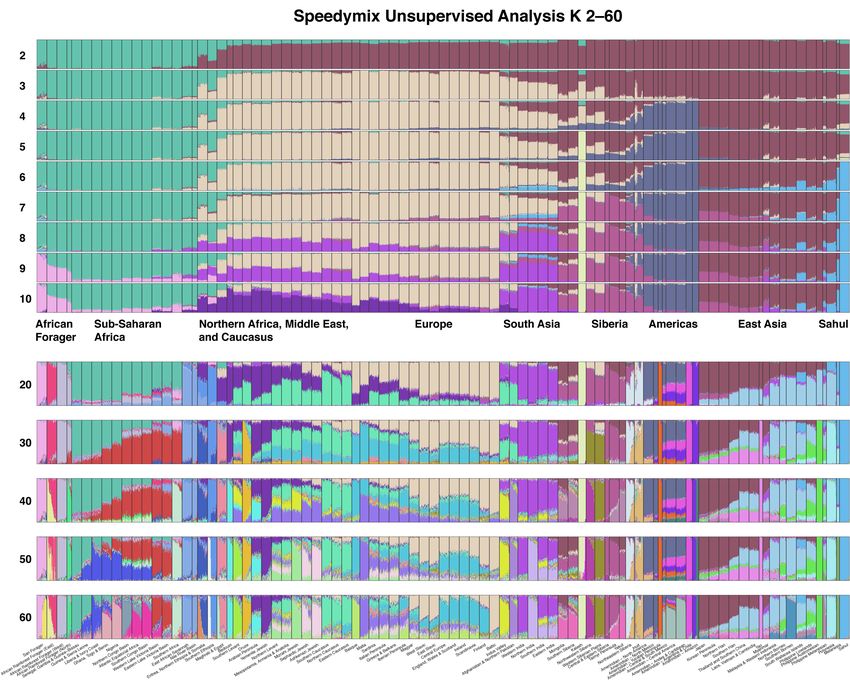
17

 San Forager
 San Forager
 Rainforest Forager African Rainforest Forager (East)
 African Rainforest Forager (North)
 African Rainforest Forager (West)
 Senegal, Gambia & Guinea-Bissau
 Guinea & Sierra Leone
 West Africa Liberia & Ivory Coast
 Ghana, Togo & Benin
 Nigeria
 Central Africa Northern Congo Basin
 Atlantic Equatorial Africa
 Southern Congo Basin
 East Africa Western Lake Victoria Basin
 Eastern Lake Victoria Basin
 South Africa Southern Africa
 Eastern Sahel East African Savannah
 Nile River Basin
 Horn of Africa Eritrea, Northern Ethiopia & Somalia
 Southern Ethiopia
 North Africa Maghreb & Egypt
 Bedouin
 Arabia Arabian Peninsula
 Yemenite Jewish
 Southern Levant
 Northern Levant
 Middle East Mesopotamia, Armenia & Anatolia
 Sephardic Jewish
 Druze
 Middle East Jewish Mizrahi Jewish
 Southern Caucasus
 Caucasus Northern Caucasus
 Eastern Caucasus
 European Jewish Ashkenazi Jewish
 Basque
 Sardinia
 Southern Malta
 Europe Iberian Peninsula
 Italian Peninsula
 Greece & Balkans
 Western Europe Central Europe
 England, Wales & Scotland
 Ireland
 Scandinavia
 Eastern Europe Magyar
 West Slavic
 East Slavic
 Baltic Baltic
 Finnish Finland
 Kalash Kalash
 West Central Indus Valley
 Asia Afghanistan & Northern Pakistan
 Western India
 Northern India
 Indian Subcontinent Southern India
 Eastern India
 Amerindian – North America
 Amerindian – North Mexico
 Amerindian – Central & South Mexico
 Amerindian – Central America
 Amerindian – Andes & Caribbean
 Americas Amerindian – Argentina & Chile
 Amerindian – Amazon
 Amerindian – Yucatan Peninsula
 Arctic Inuit
 Northeastern Siberia
 Central Siberia Yakut
 Taimyr Peninsula
 Central & Eastern Siberia
 Western Siberia Northwestern Siberia
 Western Siberian Plains
 Central Asia Southern Siberia
 Mongolia
 Myanmar Myanmar
 Northeast Asia Japan
 Korean Peninsula
 Northern Han
 Southeast Southern Han
 Asia Thailand and Southern China
 Laos, Vietnam & Cambodia
 Island Yao
 Southeast Malaysia & Western Indonesia
 Asia Philippine Lowlands
 Northern Borneo
 Philippine Southern Borneo
 South Wallacea Islands
 Indigenous Philippine Austronesian
 Philippine Melanesian
 Polynesian Polynesia
 Sahul Melanesia
 Sahul

Figure 7. Population tree for 90 MYORIGINS v3 populations from a consensus of analyses such as TreeMix,
Speedymix, hierarchical clustering on pairwise , and academic literature. The 34 super-population groupings in
MYORIGINS v3 are shown. Branch lengths have no meaning in this cladogram. Note: the true population tree of
humanity is reticulated due to admixture; however, a bifurcating tree is used here for simplicity. Therefore, this
tree is simply a clustering tool for organizing populations into super-populations and cannot accurately
reflect the complex multi-population admixtures that occurred in deeper human ancestry.

FamilyTreeDNA – MYORIGINS 3.0

18

Overview of MYORIGINS v3 Pipeline
The MYORIGINS v3 pipeline integrates the population specificity of global ancestry inference
with the genomic specificity of local ancestry inference as discussed above (see Overview). This
means we can accurately estimate the proportion of DNA a customer inherited from very specific
populations but only if genome-wide SNPs are deployed. Therefore, we do not attempt to “paint”
chromosome segments at this level of population specificity. Broader and older groups—super-
populations—contain a higher density of SNP and haplotype frequency differences, allowing us
to estimate a chromosome painting at this level in the population hierarchy.

Using dual global and local estimators has the additional benefit of combining multiple checks.
Global methods are limited by model assumptions such as the independence of SNP markers,
and therefore, undiscovered correlation between markers can slightly bias results. In contrast,
local methods make no such assumption, and in fact perform best with densely correlated SNPs
(i.e., haplotypes). We therefore expect a slight increase in accuracy by normalizing a customer’s
global ancestry proportions based on their local ancestry proportions.

Another advantage of our dual estimators is our ability to screen a customer’s populations.
Global ancestry results include a list of irrelevant populations, i.e., those with zero proportion.
This is advantageous because local methods make noisier predictions than global methods.
There is a very limited number of SNPs residing in local DNA segments, and this can cause
misclassifications. Hence, we reduce this greatly by only selecting relevant reference panels in
our local ancestry analysis.

Global and local ancestry methods in the MYORIGINS v3 pipeline are thus mutually reinforcing,
and our workflow leverages this principle (Fig. 8). Briefly, the steps are:

 • Global ancestry inference
 (1) A customer’s sample is combined with our reference panel at 379,880 SNPs.
 (2) Speedymix calculates ancestral proportions from 90 populations worldwide.
 (3) A list of relevant reference populations is selected for the next step.

 • Local ancestry inference
 (1) We phase the customer’s unphased genotype of 637,645 densely packed SNPs.
 (2) Breaking up each chromosome into small windows, segments are classified into
 relevant super-populations (out of 34 total).
 (3) A conditional random field smooths over misclassifications.
 (4) We correct phasing errors using a unique hidden Markov model.

 • Global-local ancestry integration
 (1) Globally estimated population proportions are normalized into locally estimated
 super-population proportions.
 (2) Chromosomes are sorted so that a chromosome painting may be displayed.

In the following sections, we expand on these steps in more detail.

FamilyTreeDNA – MYORIGINS 3.0

19

A B
 Speedymix
 Global
 Ancestry
 Inference Reference
 Selection

 Phasing

 Segment
 Local Classification
 Ancestry
 Inference Conditional
 Random Field Chromo.
 Painting
 (1 of 22
 Phase autosomes
 Correction shown)

 Percentages
 Global-Local Integration
 Super-Population 14%
 Population 14%
 Super-Population
 Lorem ipsum
 Lorem ipsum
 10%
 Population 10%
 ... ...
 Display Results
 Percentages and Super-Population 13%
 Chromosome Painting Population 10%
 Population 3%

Figure 8. (A) Workflow for MYORIGINS v3. See text for details. (B) Hypothetical results for a customer whose eight
great-grandparents are from different super-populations. In this example, the last great-grandparent (purple color)
comes from two different populations. Only 1 of 22 autosomes are shown for simplicity.

FamilyTreeDNA – MYORIGINS 3.0

20

Global Ancestry – Speedymix
We estimate global (genome-wide) ancestry for each customer using the references and SNP set
described above (see Finding Population Structure). Our methodology is similar to sNMF [41]
but with some important modifications—we call our software package Speedymix. The basic
idea of Speedymix (Fig. 9) is that each SNP genotype in a customer’s data ( ) exists with a
probability equal to the fraction of his/her genome that came from each population ( ),
multiplied by the frequency of that genotype in each ancestral population ( ).

 Pr( ) = (1)

Or more formally: the probability that individual possesses derived alleles at locus is
 '

 $% ( ) = 1 $& × &% ( ) , ∈ {0, 1, 2} (2)
 &()

where $& is the fraction of individual ’s genome from population , and &% is the frequency of
that genotype (either 0, 1, or 2 derived alleles; i.e., 0/0, 0/1, or 1/1) at locus in population .

This brings us to the goal: estimate a customer’s ancestry proportions ( ). Based on Equation 1,
we seek values of that minimize the difference between the most probable data Pr( ) and
the actual data ( ). This is accomplished using least-squares methods that minimize the value
 !
 LS( , ) = >| − |>* (3)

where >| |>+ is the Frobenius norm of a matrix . We use the Alternating Least Squares (ALS)
algorithm of nonnegative matrix factorization [75] to minimize the least-squares criterion in
Equation 3. We select initial values for the matrix, then iteratively estimate least-squares
values of , followed by , followed by , etc. After each cycle values of and are
normalized so all proportions and frequencies sum to 1.0. We also force all reference samples to
ancestry proportions of 1.0 in their respective populations, making the analysis semi-supervised.
The ALS algorithm alternates these cycles until it converges. This is determined by values
remaining stationary: change in ancestry proportions (

21

Local Ancestry
Phasing
Humans are diploid (2N), meaning they inherit two genomes: one maternal and one paternal.
Each haploid (1N) chromosome differs from its pair but only at a small number of positions.
These heterozygous positions are genotyped individually, e.g., A/T, C/A, G/C, without any
knowledge of the overall sequence that each parent contributed, e.g., AAG, TCC. The order of
alleles along each haploid copy of chromosomes is known as the “phase.” Phasing—or
determining the correct sequence of [ACGT] along haploid chromosomes—is essential for
conducting local ancestry analysis. Population origins of a DNA sequence cannot be determined
if the sequence is an incoherent blend of two chromosomes.

The first step in local ancestry analysis is phasing each autosomal chromosome pair. We utilize a
previously described software package called Eagle [76], which has been shown to outperform
comparable programs such as Beagle and SHAPEIT, particularly when using large reference
panels [77]. A large panel of unrelated individuals is essential for accurate phasing, and we use
our 100K phasing panel. Eagle combines two different techniques for phasing: (1) searching a
reference panel for short haplotypes that are exact matches (i.e., distant cousins that share DNA
identical-by-descent (IBD) from a common ancestor); (2) modeling haplotype frequency in the
panel to calculate the probability of each possible haplotype (Fig. 10). Eagle combines these two
techniques for increased computational speed and accuracy.

The Eagle algorithm contains three steps to phase a chromosome:

 (1) It scans the reference panel for >4 cM matching segments, i.e., those matching at least
 one allele at every SNP. Potential matches are scored according to their likelihood of
 being close or distant relatives (and not matching due to chance). All matches above a
 threshold likelihood score are then pruned to remove any matches that are
 inconsistent with other matches. Finally, phase is assigned to a customer’s genotype
 using the IBD matches. For every SNP that is heterozygous in the customer, a
 homozygous match is used to determine phase. If the SNP is heterozygous in all
 matches, then allele frequency is used to phase the SNP probabilistically.

 (2) It splits the chromosome into overlapping windows of approximately 1 cM, and once
 again, scans the reference panel for matches. This time it finds the best pair of
 complementary matches for both maternal and paternal haplotypes in the customer’s
 sample. The idea is to vastly increase the number of potential matching segments by
 allowing extremely distant relationships (e.g., 1 cM may be shared by 20th cousins).
 Several SNP mismatches are tolerated in this step to accommodate phasing errors
 from Step 1. The pair of complementary matches with fewest errors is used to locally
 refine the customer’s phase in each window.

 (3) Finally, it models haplotype frequency and recombination in the reference panel to
 statistically phase sites that were not adequately phased in the first two steps. Using
 up to 80 reference matches that represent both maternal and paternal haplotypes, it

FamilyTreeDNA – MYORIGINS 3.0

22

 phases 0.3 cM windows with a Hidden Markov Model (HMM). The model is based
 on a previously described model of recombination [78], which exploits the fact that
 unknown haplotypes are likely to be similar to frequently occurring haplotypes.
 Therefore, the HMM chooses appropriate references to phase the customer’s sample
 by penalizing recombination and mutation between the two matches. Two iterations
 of the Viterbi algorithm are used to find the most likely haplotype phase of the HMM.

The end result of Eagle phasing is a set of SNP genotypes on each chromosome with maternal
and paternal alleles separated into different haplotypes. Although Eagle phasing is ~99.7%
accurate, it cannot be perfect. There are still switch errors (maternal/paternal transitions)
approximately every few cM [76]. Since local ancestry methods classify tiny DNA segments that
are much smaller than this, switch errors have little effect on the final ancestry proportions.
However, at the end of the local ancestry pipeline, these switch errors must be corrected by using
the inferred sequence of super-population ancestry (see Phase Correction).

 Distant IBD
 Relative Match
 A /C A
 ? ?
 G /G G
 ? ?
 C/T C
 ? ?
 T /T T
 ? ?
 A /A A
 ? ?
 Unphased G /G G Phased
 ? ? Genotypes Genotypes
 ? ? A /A A |A
 ? ? T /G G|T
 ? ? C /C C |C
 ? ? T /T T |T
 ? ? A /C A |C
 ? ? G /G Possible Possible G |G
 ? ? Phasing 1 Phasing 2
 ? ?
 A A A A
 G T T G
 C C C C
 T T T T
 A C A C
 G G G G
 Population Frequency
 45% 35% 15% 5%
 {
 {

 95% 5%
 Probability
Figure 10. Eagle combines two different methods of phasing: exact IBD matches (top) and haplotype frequencies in
a reference panel to generate phasing probabilities (bottom).

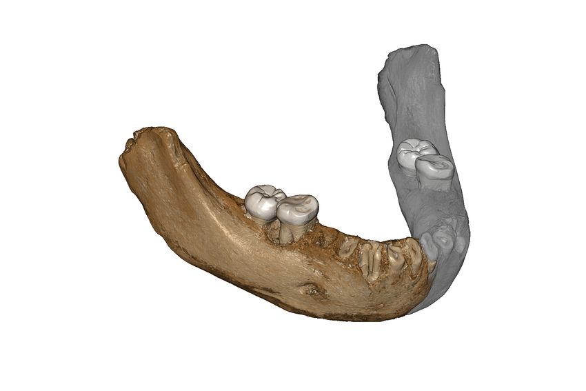
FamilyTreeDNA – MYORIGINS 3.0

23

Segment Classification
Local ancestry inference (LAI) is a method for determining population ancestry along small
segments of each chromosome. In contrast to a global ancestry method such as Speedymix,
which can only determine overall ancestry proportions, LAI can also determine the genetic
coordinates where each ancestral population segment was recombined. Chromosome painting is
somewhat synonymous with LAI but generally refers to the result instead of the method.

LAI has existed for nearly two decades and was originally designed as an extension of the most
popular global ancestry method [19]. The idea behind LAI is to leverage the correlation between
SNP markers that are in close proximity to one another. Recombination cannot fully break up the
association between adjacent SNPs over shorter time intervals, a phenomenon known as linkage
disequilibrium. Hence, the order of SNPs along a DNA segment can be highly informative about
its population origin. Short segments of DNA that are shared by many individuals in a particular
population due to ancient shared ancestry are known as identical-by-state (IBS).

Some of the earliest applications of LAI were to identify locations of genes associated with
human diseases, a process known as admixture mapping [15,20,21]. However, the method has
also continually been refined in order to study human admixture proportions or measure the
amount of time elapsed since admixture. Over two dozen methods of LAI now exist [12–36].
Very often, a Hidden Markov Model (HMM) or one of its derivatives is used to model ancestry
as a hidden state, based on either the observed order of SNPs or haplotypes [15,19–21].
Sometimes, other classification methods are used in conjunction with or instead of an HMM:
e.g., Markov chain Monte Carlo [19,21,30], iterated conditional modes [16], PCA [24,30],
random forests [33], dynamic programming [14], and deep learning [28].

In MYORIGINS v3 we classify phased haplotype segments with our own proprietary machine
learning technique (Fig. 11). We have found it to outperform one of the most popular LAI
methods [33]. We break a customer’s phased chromosomal data into segments of 500 SNPs in
overlapping windows spaced apart by 200 SNPs. Then, we classify each segment into one of
several super-populations using a multi-class clustering method. Our technique is ideal for
discriminating between groups with data that are complex and high-dimensional (such as SNP
haplotypes). We use the same reference panel as in Speedymix except all references are phased
at the full set of 637,645 SNPs.

Our pipeline is novel and unique in its paired use of global and local estimates. Due to the
inherently noisy nature of LAI, which must classify small segments with limited information,
super-populations are used instead of populations. Using groups that are older and more distinct
allows us to more accurately classify segments. Unlike other existing LAI methods, ours reduces
noise in results by eliminating irrelevant super-populations during the Speedymix step.
Additionally, we apply weights ( ) for each relevant super-population to correct for sample size
imbalance: & = /( & ), where & is the sample size of class , and is the total number of
classes. The super-population confidence scores are mapped into probabilities using a sigmoid
function to be used in the next step of our pipeline.

FamilyTreeDNA – MYORIGINS 3.0

24

A B
 Pop1:

 200 SNP
 Pop2:
 Window
 Spacing
 SNP:

 500 SNP
 Segment C y
 Classification

 x
 * window size not to scale

Figure 11. Segment classification steps. (A) Each pair of phased chromosomes is divided into windows spaced 200
SNPs apart, and overlapping segments of 500 SNPs are taken from each window for classification. (B) ACGT letter
size represents frequency of that nucleotide in hypothetical super-populations 1 and 2 along a 500 SNP haplotype.
Haplotype differences between super-populations are quantified and modeled. (C) Our proprietary classification
technique is trained on all super-populations to maximize the distance between them in multi-dimensional space.
The star indicates a customer sample that was predicted into hypothetical super-population 1.

FamilyTreeDNA – MYORIGINS 3.0

25

Conditional Random Field
Once each segment of each chromosome is assigned probabilities of each super-population, we
use those probabilities to parameterize a linear chain conditional random field (CRF). This
process uses pattern recognition of an entire chromosome to better predict the sequence of
ancestries. The CRF “smooths over” each segment classification by incorporating information
from neighboring segments on the chromosome. Although the small number of SNPs available
to segment classifiers can result in more noise (Fig. 2C), the CRF step adjusts misclassifications
by maximizing the probability of the entire sequence (Fig. 12). Our linear-chain CRF follows
[33] except that our segment probabilities are estimated by our method instead of random forests.

For each chromosome, we model the ancestries of individual haplotypes {1. . . } across 200 SNP
windows {1. . . } as an × matrix , where $,- is the most probable super-population ∈
{1. . . } for individual at window . Similarly, we model all haplotypes as an × matrix ,
where $,- is the haplotype ℎ for individual at window .

The log-linear probability of ancestries across individual ’s entire haploid chromosome is

 PrK $,∗ > $,∗ : ΘN = (4)

 6 ' 67) ' '
 1 0 #
 exp S1 1 1 -,&,/ 110&,( (&2 113&,( (/2 + 1 1 1 -,&,& ) 110 1 ) V
 &,( (&2 10&,(*+ (& 2
 K $,∗ N
 -() &() /∈ℋ( -() &() & ) ()

where ℋ- includes all possible haplotypes in window w, 1{9(:} equals 1 if = and 0
otherwise, and K $,∗ N is a partition function for normalizing the probability:

 K $,∗ N = (5)

 6 ' 67) ' '
 0 #
 1 exp S 1 1 1 -,&,/ 11
 -,&,& ) = ( ( $,- = , __ $,-=) = ))
 (7)
Parameter values of 0 are estimated by the multi-class segment probabilities (previous step),
whereas the # values are estimated by a previously described [19] linkage model of admixture:

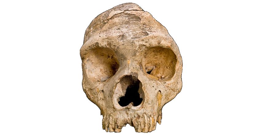
FamilyTreeDNA – MYORIGINS 3.0

26

 ( (− - ) + (1 − (− - )) & ) ) if = > (8)
 PrK $,- = , $,-=) = > N = a &
 & ((1 − (− - )) & ) ) otherwise

where - is the distance between the midpoints of windows and + 1, is the number of
generations since admixture, and & and &> are the chromosome-wide admixture proportions for
the super-population in the current window ( ) and the next window ( > ).

The logic for this linkage model is as follows. Recombination is responsible for breaking apart
and fusing together DNA haplotypes from different super-populations. One breakpoint does not
influence the location of a future breakpoint; thus, recombination can be modeled as a random
Poisson process. The term can be thought of as the expected number of recombination events
within the window since admixture occurred. The top portion of equation (9) accounts for the
possibility that no recombination has occurred in the window, or there has been at least one
breakpoint but with the adjacent windows coming from the same super-population. The bottom
portion of equation (9) accounts for the possibility of at least one breakpoint, resulting in a
switch from super-population to > . We use a uniform distribution for values of & to simplify
the model, although chromosome-wide admixture proportions could be included in the future.

For each customer’s haploid chromosomes, we use the Viterbi algorithm along with the CRF
probability to infer the most likely chain of ancestries.

 CRF

Figure 12. Effect of the Conditional Random Field: noisy classifications are “smoothed out” by a linkage model.

FamilyTreeDNA – MYORIGINS 3.0

27

Phase Correction
Statistical phasing is >99% accurate, but this small minority of switch errors add up across
100,000s of SNP positions. Fortunately, the end result can be corrected by essentially “phasing”
the final super-population labels. We use a Hidden Markov Model (HMM) parameterized by
some basic expectations of which pair of maternal/paternal labels are most probable in each
window, given the labels in the previous window (Fig. 13). Phase correction, the removal of
switch errors using an HMM, is nearly as old as local ancestry inference itself [13,14,28,33].

First, we initialize the space for hidden states and observations. For each window along a
chromosome, the observation is a diploid pair of predicted super-population labels, and the
hidden state is the true pair of super-population labels. If a customer’s result includes proportions
from super-populations, then the observation space / > and hidden state space / > are both
pairs of super-population labels where , > , , > ∈ {1. . . }.

We assume that all observations are potentially unphased but contain the correct labels.
Therefore, our HMM model only allows the chromosome strands to be flipped. The emission
probabilities of observed states given hidden states is:

 0.5 if ( = and > = > ) or ( = > and > = ) (9)
 PrK $$ ) | ?? ) N = n
 0 otherwise

To illustrate this: when label pair 1/2 is observed, the hidden state for it can only be 1/2 or 2/1
with equal probabilities.

The main correction comes from our transition probabilities. Recombination happens rarely
compared with the number of windows, so we assign higher probability for hidden states to
belong to the same chromosome strand:

 PrK $$ ) ,- | ?? ) ,-7) N = (10)
 if ( = and > = > )
 ⎧ )
 ⎪0 if ( = > and > = )
 (1 − ) ) ! if ( = and ≠ ) or ( = > and ≠ > )
 >
 ⎨ (1 − )(1 − ) if ( = > and ≠ > ) or ( = > and ≠ > )
 ⎪ ) ! @
 ⎩ (1 − ) )(1 − ! )(1 − @ ) if ( ≠ and ≠ ′) or ( ≠ > and ≠ > )

where ) = 0.85, ! = 0.85, and @ = 0.75 (see Table 3).

Table 3. Transition probabilities for each type of change between diploid pairs of super-population labels.

 Type Example Probability
 No change 1/2 to 1/2 0.85
 Strand flip 1/2 to 2/1 0.00
 Partial overlap 1/2 to 1/3 0.1275
 Partial overlap after strand flip 1/2 to 3/1 0.016875
 Other 1/2 to 3/4 0.005625
 Total 1.00

FamilyTreeDNA – MYORIGINS 3.0