Nested association mapping reveals the genetic architecture of spike emergence and anthesis timing in intermediate wheatgrass
←
→
Page content transcription
If your browser does not render page correctly, please read the page content below
2
                                                                                                                                    G3, 2021, 11(3), jkab025
                                                                                                                          DOI: 10.1093/g3journal/jkab025
                                                                                                          Advance Access Publication Date: 30 January 2021
                                                                                                                                Multiparental Populations

Nested association mapping reveals the genetic
architecture of spike emergence and anthesis
timing in intermediate wheatgrass
                     1
                      *, Steven R. Larson2, Lee R. DeHaan3, Jared Crain                     4                      5
                                                                                                                    , Kevin M. Dorn6, and

                                                                                                                                                                  Downloaded from https://academic.oup.com/g3journal/article/11/3/jkab025/6124305 by guest on 12 December 2021
Kayla R. Altendorf                                                                            , Jeff Neyhart
                   7
James A. Anderson
1
  USDA-ARS, Forage Seed and Cereal Research Unit, Irrigated Agriculture Research and Extension Center, Prosser, WA 99350, USA
2
  USDA-ARS, Forage Range and Research Lab, Utah State University, Logan, UT 84322, USA
3
  The Land Institute, Salina, KS 67401, USA
4
  Department of Plant Pathology, Kansas State University, Manhattan, KS 66506, USA
5
  GEMS Informatics Initiative, University of Minnesota, St. Paul, MN 55108, USA
6
  USDA-ARS, Soil Management and Sugarbeet Research, Fort Collins, CO 80526, USA
7
  Department of Agronomy and Plant Genetics, University of Minnesota, St. Paul, MN 55108, USA

*Corresponding author: Irrigated Agriculture Research and Extension Center, 24106 North Bunn Road, Prosser, WA 99350, USA. kayla.altendorf@usda.gov
Mention of trade names or commercial products in this publication is solely for the purpose of providing specific information and does not imply recommendation
or endorsement by the U.S. Department of Agriculture. USDA is an equal opportunity provider and employer.

Abstract
Intermediate wheatgrass (Thinopyrum intermedium) is an outcrossing, cool season grass species currently undergoing direct domestication
as a perennial grain crop. Though many traits are selection targets, understanding the genetic architecture of those important for local
adaptation may accelerate the domestication process. Nested association mapping (NAM) has proven useful in dissecting the genetic con-
trol of agronomic traits many crop species, but its utility in primarily outcrossing, perennial species has yet to be demonstrated. Here, we
introduce an intermediate wheatgrass NAM population developed by crossing ten phenotypically divergent donor parents to an adapted
common parent in a reciprocal manner, yielding 1,168 F1 progeny from 10 families. Using genotyping by sequencing, we identified 8,003
SNP markers and developed a population-specific consensus genetic map with 3,144 markers across 21 linkage groups. Using both
genomewide association mapping and linkage mapping combined across and within families, we characterized the genetic control of flow-
ering time. In the analysis of two measures of maturity across four separate environments, we detected as many as 75 significant QTL,
many of which correspond to the same regions in both analysis methods across 11 chromosomes. The results demonstrate a complex ge-
netic control that is variable across years, locations, traits, and within families. The methods were effective at detecting previously identified
QTL, as well as new QTL that align closely to the well-characterized flowering time orthologs from barley, including Ppd-H1 and Constans.
Our results demonstrate the utility of the NAM population for understanding the genetic control of flowering time and its potential for ap-
plication to other traits of interest.

Keywords: Nested association mapping; intermediate wheatgrass; flowering time

Introduction                                                                       Rodale Institute (Kutztown, PA, USA) in the early 1980s sur-
Intermediate wheatgrass (Thinopyrum intermedium; (Host)                            veyed over 100 perennial grasses for their domestication poten-
Barkworth& D.R. Dewey; IWG hereafter) is a perennial, cool-                        tial (Wagoner 1990). They selected IWG due to its relatively
season grass undergoing direct domestication as a dual-use                         large seed size, nutritional similarity to wheat, perennial
forage and grain crop for human consumption (DeHaan et al.                         growth, and its ability to be mechanically harvested. Initial
2014). IWG is primarily self-incompatible, outcrossing allohex-                    germplasm surveys began in 1987 (Wagoner 1990) after which,
aploid (2n ¼ 6x ¼ 42) (Dewey 1962). Native to Europe and Asia,                     breeding and domestication programs were established at The
it was introduced to North America in 1932 and has since been                      Land Institute (TLI; Salina, KS; DeHaan et al. 2018), the
used primarily as a hay and pasture grass (Dewey 1962; Ogle                        University of Minnesota (Zhang et al. 2016), the University of
et al. 2011) and a source disease resistance genes for common                      Manitoba (DeHaan et al. 2014), and new programs have been
wheat (e.g., Brettell et al. 1988; Friebe et al. 1996; Turner et al.               initiated in Utah and Internationally in Europe in the last few
2013). Citing the need for perennial crops to improve agricul-                     years. These programs utilize phenotype-, pedigree-, or
tural sustainability on highly erodible or marginal lands, the                     genotype-based recurrent selection and cultivars are developed

Received: September 25, 2020. Accepted: January 07, 2021
C The Author(s) 2021. Published by Oxford University Press on behalf of Genetics Society of America.
V
This is an Open Access article distributed under the terms of the Creative Commons Attribution License (http://creativecommons.org/licenses/by/4.0/), which
permits unrestricted reuse, distribution, and reproduction in any medium, provided the original work is properly cited.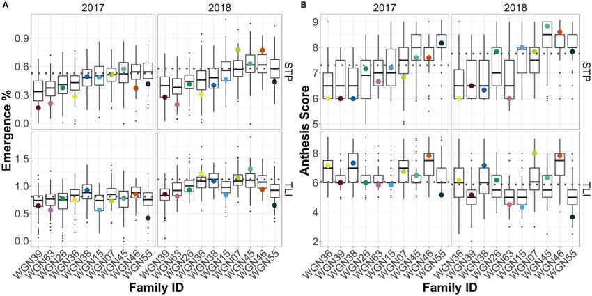
2   |   G3, 2021, Vol. 11, No. 3

as synthetics (DeHaan et al. 2014; Zhang et al. 2016; Bajgain           frequency and sampling of rare alleles in both common and do-
et al. 2020a, b; Crain et al. 2020).                                    nor parents that may otherwise go undetected or filtered out due
    Despite the many genetic resources developed for IWG, and           to a minimum minor allele frequency (MAF) threshold. Finally,
some early selection success, breeding targets remain vast. IWG         crossing wild or unadapted donor parents with a highly adapted
has a dense genetic consensus map with 10,029 markers from              common parent allows for the assessment of diverse germplasm
seven full-sib families (Kantarski et al. 2016), an optimized proto-    (Poland et al. 2011; Nice et al. 2017).
col for developing genotyping-by-sequencing (GBS) libraries                Contrary to an inbred NAM, an F1 NAM requires special con-
(Elshire et al. 2011; Zhang et al. 2016), and a draft reference ge-     siderations with regards to the segregation of alleles. For exam-
nome under development by the T. intermedium Genome                     ple, bi-parental families can segregate from anywhere between 2
Sequencing Consortium (DeHaan et al. 2018; Larson et al. 2019).         and 4 alleles, and this number can vary across loci (Van Ooijen
Breeding and selection have primarily focused on increasing seed        2011). Thus, it is not possible to observe allele combinations in
size and yield on a per spike basis (DeHaan et al. 2018) and despite    homozygous, identical-by-descent states as it is in an inbreeding

                                                                                                                                                 Downloaded from https://academic.oup.com/g3journal/article/11/3/jkab025/6124305 by guest on 12 December 2021
the infancy of breeding efforts, gains from selection have been         species. Because the parents are segregating, imputation of
observed. For example, after 5 cycles of selection at TLI, a 143%       densely genotyped parents on progeny is difficult, and diverse do-
increase in yield per spike and a 60% increase in seed mass was         nor alleles cannot be assessed relative to a common genetic back-
predicted (observed response would require evaluation in the            ground. Many computational programs developed for NAMs and
same environment) in a spaced plant setting (DeHaan et al. 2018).       other multi-parent populations, including the R packages “NAM”
Furthermore, genomic selection has shown great promise in               (Xavier et al. 2015), “mppR” (Garin et al. 2107), and “R/qtl2”
IWG, demonstrating high-predictive ability (in one study, r¼ 0.46       (Broman et al. 2019), all depend on homozygous parents and prog-
– 0.67; depending on the trait, and > 0.5 in another) and has im-       eny to reconstruct haplotypes and phasing and are not suited for
proved the precision and efficiency of selection (Zhang et al. 2016;    heterozygous parents. In some cases, heterozygous sites within
Crain et al. 2021). Including significant markers from QTL map-         the parents and progeny are excluded from the analysis, which
ping studies as co-factors in genomic selection models has been         would likely result in significant data loss in the case of an out-
shown to increase predictive ability and increases the frequency        crossing species. Finally, it is important to note that instead of
of favorable alleles (Zhang et al. 2017; Bajgain et al. 2019a, b).      maximizing genetic divergence between parental material, as
However, IWG is still susceptible to seed shattering (Larson et al.     would be the case in a traditional NAM, the objective instead is to
2019), has low threshability (Zhang et al. 2016), is tall and prone     maximize heterozygosity within parents to observe segregation
to stem lodging (Frahm et al. 2018), and has low-floret site utiliza-   among the progeny. These challenges can be overcome by using
tion that may contribute to low yields (Altendorf et al. 2020). An      programs and methods designed for phasing and mapping in out-
improved understanding of the genetic architecture of these im-         crossing species, such as JoinMap and MapQTL (Van Ooijen 2009;
portant traits has the potential to further increase efficiency and     2011). Considering the demonstrated utility of the population de-
precision in IWG breeding efforts through genomics assisted             sign and the need within the IWG breeding community to assess
breeding, but the difficulty lies in the fact that relatively few       the genetic control of many traits of interest, a NAM population
marker-trait association studies have been conducted in IWG             is worth exploring.
and the genetic control of many important traits remains poorly            Here, we introduce an IWG NAM population and assess its
understood.                                                             utility by dissecting the genetic control of flowering time. The
    Nested association mapping (NAM) was developed to combine           timing of the transition from vegetative to reproductive phases is
the benefits of both linkage and association mapping by crossing        a critical step to ensure proper timing for pollination, seed set
one common parent with a series of diverse donor parents and            and dispersal, and variation for this trait has played a critical role
developing segregating populations in the form of recombinant           in the adaptation of crops to new growing environments
inbred lines (RILs; Yu et al. 2008). This approach has demon-           (Cockram et al. 2007). The objectives of this work were to: (1) de-
strated utility in many crop species including maize (Buckler et al.    velop and genetically characterize an IWG NAM population; (2)
2009; McMullen et al. 2009), rice (Fragoso et al. 2017), wheat          describe the phenotypic variation in the NAM for flowering time
(Bajgain et al. 2016; Jordan et al. 2018; Wang et al. 2019), barley     over 2 years in two distinct locations: St. Paul, MN, and Salina,
(Maurer et al. 2016; Nice et al. 2017; Hemshrot et al. 2019), sorghum   KS; (3) assess the genetic control of flowering time using two
(Bouchet et al. 2017), and soybean (Song et al. 2017). Notably, all     approaches: GWAS and linkage mapping within and across mul-
the aforementioned species are self-compatible where the devel-         tiple populations. The linkage mapping method accurately
opment of RILs is possible and commonplace. To our knowledge,           assesses the within family allele effects by utilizing phasing and
there have been no formally published NAMs developed in an              tracing the parental origin of 2–4 alleles at a locus. The GWAS ap-
outcrossing, self-incompatible species, nor for any cool season,        proach serves as additional support for QTL identification, and
perennial grasses (Talukder and Saha 2017).                             results are compared across both methods.
    In an outcrossing, self-incompatible species, the NAM design
still includes common and donor parents, but eliminates the RIL
development step, and all progeny are F1 and therefore highly
                                                                        Materials and methods
heterozygous and heterogeneous. While this may result in a de-          Population development and establishment
crease in mapping resolution due to the lack of recombination           Ten phenotypically diverse genets (donor parents) and one low-
and breakdown of LD associated with inbreeding, there are vari-         shattering genet (common parent) were identified from Cycle 2 of
ous practical advantages NAM that may be realized. First and            the University of Minnesota breeding program based on their
foremost, multiple parents offer more genetic variation and in-         traits of interest (Table 1). Genet refers to plants of the same ge-
crease the utility of a population by allowing the dissection of        netic makeup, with multiple clones of each genet are referred to
more than a single trait compared with a traditional bi-parental        as ramets. This terminology is consistent with Zhang et al. (2016)
mapping population. Second, relative to genome wide association         and accounts for the heterozygous nature of IWG as the terms
study (GWAS) in diverse populations, NAM offers increased               line or cultivar would be inconsistent with normal usage in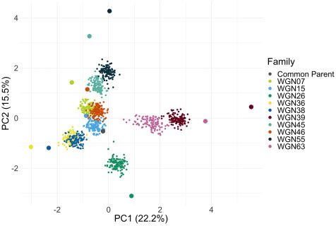
K. R. Altendorf et al.    |   3

Table 1 Families of the intermediate wheatgrass nested association mapping population, their family sizes separated by maternal
parent, and their phenotypic characteristics as recorded in historical breeding program data from St. Paul, MN, which served as the
basis of their initial selection

                                   Family sizea and maternal parent                                          Phenotypic characterization

Parent       Parent type         Common              Donor           Total         Heading        Height (cm)       Seed size (mg)    Shattering    Threshability
                                                                                  date (1–5)b                                           (0–4)c         (1–9)d

WGN07        Donor                   59                62             121              3                75                  6.83           1               7
WGN15        Donor                   60                60             120              5               130                  8.88           0               6
WGN26        Donor                   62                59             121              3               135                 12.52           3               1
WGN36        Donor                   51                63             114              3               103                 10.1           0.5              4
WGN38        Donor                   66                29              95              2                77                  9.1            1              0.5
WGN39        Donor                   59                63             122              3               131                  9.5            3               3

                                                                                                                                                                        Downloaded from https://academic.oup.com/g3journal/article/11/3/jkab025/6124305 by guest on 12 December 2021
WGN45        Donor                   54                64             118              —               120                 10.58          0.5              5
WGN46        Donor                   58                63             121              —               108                  8.28           3               6
WGN55        Donor                   61                62             123              —               111                 10.48           3               6
WGN59        Common                  —                 —               —               —               131                 10.56          0.5              7
WGN63        Donor                   57                56             113              —               126                  9.18           3               1
 a
     Determined by samples for which there is both phenotypic and genotypic data.
 b
     Historical data on the heading date was not available for all parents, where one is late and five is early heading.
 c
     Shattering scale, where zero is low and four is high.
 d
     Threshability scale, where zero is low and nine is high.

inbred crops. Parents, and therefore families, were named after                        successful establishment. Plots were hand weeded and cultivated
their numerical designation within the IWG breeding program                            with a multivator (Ford Distributing, Marysville, OH, USA) as nec-
preceded with “WGN” for “Wheatgrass NAM.” Parental genets                              essary to control weeds. In addition, a pre-emergent herbicide,
were propagated from the field in Fall 2015 into 3–5 clones                            Dual II Magnum (S-metolachlor, Syngenta US), was applied at
each, planted in 3.8 L pots, and allowed to re-establish in the                        STP in April 2017 and May 2018 at a rate of 1.75 L ha1. Herbicides
greenhouse before vernalization at 4 C for 2 months. After ver-                       were not used at TLI. At both locations, plots were mowed to
nalization, plants were placed in a growth chamber (16 hour day,                       15 cm height after harvest and fertilized with urea (56.0 kg ha1
18–20 C) to induce flowering. In May 2016, multiple reciprocal                        at STP; 78.5 kg ha1 at TLI) in fall 2017. Forty-four ramets died be-
crosses were made between each donor parent and the common                             tween transplanting and the end of the 2017 harvest season at
parent by bagging spikes together in custom pollination bags (PBS                      TLI, and 25 additional ramets died in the 2018 field season. An
International, UK) just before pollen shed. Spikes from each cross                     additional 203 ramets at TLI were deemed not worth harvesting
were harvested in July 2016 and kept separate on the basis of                          in 2018 due to drought conditions. In St. Paul, 76 ramets were lost
family and maternal parent identity. Spikes were threshed and                          between transplanting and harvesting in 2017, and an additional
cleaned using a belt thresher, sieve (12/64” round; SEEDBURO,                          2 in 2018.
Des Plaines, IL, USA) and aspirator (Air Blast Seed Cleaner;
ALMACO, Nevada, IA, USA). Approximately 150 seeds from each                            Growing degree days
cross (75 from each maternal parent) were placed on moist blot-                       Weather data for St. Paul was obtained from National Oceanic
ter paper (Anchor Paper, St. Paul, MN, USA) in petri dishes and                        and Atmospheric Administration (NOAA, RRID: SCR_011426)
subjected to a cold treatment of 4 C for 3–5 days or until germina-                   from the St. Paul Agricultural Experiment Station (Station ID:
tion occurred. Germinating seeds were transplanted at 1 cm                             USC00218450). Weather data for Salina, KS was obtained from
depth into 10 cm 21-count trays and placed in a misting green-                         the TLI Weather Station. Growing degree days (GDDs) were calcu-
house for 4 days and then transferred to an outdoor nursery.                           lated in degrees Celsius using the following equation, where Tmax
Plants were watered daily and fertilized weekly with a standard                        and Tmin are the maximum and minimum daily temperatures,
solution (15 mL per 4.4 L) of 20-20-20 fertilizer, and monthly with                    and Tbase is 0 C, or the base temperature for growth used in IWG
slow-release Osmocote (The Scotts Company, Marysville, OH,                             (Frank 1996; Jungers et al. 2018):
USA). In August, plants were clipped to 5 cm to promote tiller-
ing, propagated into four ramets per genet and placed into 5                                                    ½ðTmax þ Tmin Þ =2  Tbase
5 cm peat pots (Plantation Products, Norton, MA, USA) in
September. Genets were completely randomized within blocks                                A maximum threshold of 37 C was set for Tmax, which is the
and were transplanted into spaced plant nurseries in a random-                         predicted maximum temperature for growth in wheat (Porter and
ize complete block design (RCBD) with two blocks at the                                Gawith 1999), and GDD accumulation began and ended after 5
University of Minnesota Agricultural Experiment Station in St.                         consecutive days where the average daily temperature exceeded
Paul, MN, USA (1-m centers; STP hereafter) using a mechanical                          Tbase (Frank and Hoffman 1989).
transplanter on 30 September, and at The Land Institute in
Salina, KS (0.9-m centers; TLI hereafter) using a jab-type planter                     Phenotypic data collection
on 16 October. The genets, or spaced plants, were considered the                       Two measures of reproductive growth stage were recorded: spike
experimental units. Several clones of each donor parent (3 per                        emergence percent and anthesis stage. IWG spike length is vari-
block) and the common parent (25 per block) were included and                         able both within and among genets, making it challenging to vi-
a two-plant border was established to limit edge effects.                              sually estimate the proportion of the spike that has emerged
Transplants were watered once after transplanting to promote                           from the boot as is done in a traditional maturity rating scale
4 | G3, 2021, Vol. 11, No. 3
such as BBCH, Feekes, or Zadoks (Large 1954; Zadoks et al. 1974; Genotyping-by-sequencing
Lancashire et al. 1991). Thus, to more precisely capture variation Young leaf tissue was harvested from each genet prior to plant-
in emergence time, when spikes were approximately 50% ing, freeze dried, and genomic DNA was extracted using the
emerged on average across the population, the length of the spike BioSprint 96 Plant DNA Kit (QIAGEN, the Netherlands). DNA was
emerged from the boot (from the tip of the most apical spikelet to quantified using QuantiFluor dsDNA System (Promega
the base of the flag leaf) was measured in cm on one spike per Corporation, WI, USA) and normalized to 10 ng/ml. Genotyping by
plant. As maturity within a plant can vary, especially in the first sequencing libraries were developed using PstI/Msp I enzymes fol-
year, larger, more uniform spikes were chosen for measurement lowing Zhang et al. (2016) with two barcodes per sample. Every 96
to minimize experimental error (DeHaan et al. 2018). In cases of samples were pooled, creating a total of fifteen 96-plex libraries.
high within-plant variability (e.g., 5 cm), the mean of two spikes The common parent was sampled eight times and the donor
was recorded. Harvesting procedures were previously outlined in parents six each to achieve higher sequencing depth. Libraries
Altendorf et al. (2020). After harvest, three spikes were aligned were amplified and cleaned using the QIAquick PCR Purification
Downloaded from https://academic.oup.com/g3journal/article/11/3/jkab025/6124305 by guest on 12 December 2021
end-to-end (from tip of most apical spikelet to base of the most Kit (QIAGEN, the Netherlands), quality control was done using
basal spikelet, a spikelet defined as having glumes and at least Picogreen (ThermoFisher Scientific, MA, USA), Agilent
one floret) along a measuring tape and total length was recorded Bioanalyzer (Agilent, CA, USA) and Kapa qPCR, and subjected to
and divided by three to obtain the mean. Length emerged divided size selection of 160–240bp using PippinHT (3% agarose). Each
by final spike length represents percent spike emergence. In pool was sequenced in a single lane of a 100 bp single read run on
cases where the spike was completely emerged, the length of the the Illumina HiSeq 2500 HO using v4 chemistry at the University
emerged peduncle was included, resulting in some estimates ex- of Minnesota Genomics Center.
ceeding 100%. Early spike emergence is not always coupled with
early anthesis in IWG (personal observation). Thus, Feekes flow-
ering time was also recorded for each plant on one occasion per Variant detection and filtering
environment when anthers were showing (approximately Fastq files from the sequencer were demultiplexed using the
1600–1800 hour) and when approximately 50% of the plants were Barcode Splitter tool from the FastX-Toolkit (RRID: SCR_005534)
in anthesis (Large 1954). Categories were coded as ordinal varia- where barcodes were matched at the beginning of reads and no
bles for data analysis and included: (1) boot stage where no spike mismatches were allowed. Read quality was assessed using
is visible; (2) heads emerging or < 25%; (3) heading 25%; (4) head- FastQC (RRID: SCR_014583). Adapter sequences, designed accord-
ing 50%; (5) heading 75%; (6) heading complete but no anthers ing to (Poland et al. 2012), were removed using CutAdapt (Martin,
visible; (7) beginning flowering, where yellow anthers are begin- 2011; RRID: SCR_011841). The Quality Trimmer tool from FastX-
ning to emerge at the center of the spike; (8) flowering 50%, where Toolkit was used to trim reads with a quality score less than 30
anthers are visible through the center and top of spike; (9) flower- (phred þ 33 scale) and a minimum read length of 30 (-Q 33 -t 30 -l
ing 100% where anthers (possibly white or dehiscing) are visible 50 -v). After adapter removal and read trimming, quality was
throughout the entirety of the spike including the most basal confirmed by re-running FastQC. Bowtie2 (Langmead and
spikelets; and (10) kernels watery ripe, where anthers are likely Salzberg, 2012; RRID: SCR_055476) was used to align reads to v2
dehisced and florets appear plump. The same person recorded of the draft IWG reference genome (access provided by The
anthesis across all locations and years. Dates of data collection T. intermedium Genome Sequencing Consortium), which was
events are reported in Supplementary Figure S1. indexed prior to analysis. Options were set to require reads to
align entirely and the very-sensitive preset was used, with zero
ambiguous reference characters. Reads were filtered to include
Phenotypic data analysis only those that mapped uniquely to the reference, and files were
All phenotypic data analyses were conducted in R v3.6.1 (R Core sorted and indexed using SAMtools (Li et al. 2009; RRID:
Team 2020). In a separate analysis of yield component traits, we SCR_002105). Within each lane, fastq files with barcodes corre-
previously reported the calculation of estimated marginal means sponding to the same sample were concatenated using a custom
(“emmeans”) for each genet nested within family for both spike BASH script. The Genome Analysis Toolkit (GATK) v4.1.2
emergence percent and anthesis, as well as correlations between (McKenna et al. 2010; RRID: SCR_001876) was used to call var-
traits, and both broad and narrow sense heritability estimates iants, beginning with the HaplotypeCaller tool, which was set to
(Lenth 2018; Altendorf et al. 2020). Because an initial linear model eliminate the duplicate read filter, run in GVCF mode and with
analysis across environments revealed highly significant interac- an expected heterozygosity rate of 0.01. GATK required a dictio-
tions, we analyzed all unique year by location combinations (n ¼ nary and an “fai” index of the reference genome; these were cre-
4; environments hereafter) separately. This decision was further ated using the GATK “CreateSequenceDictionary” and the
supported by differences in plant age between 2017 and 2018, as SAMtools “faidx” commands, respectively. The CombineGVCF
well as major differences in climate and GDD accumulation be- tool was used to merge individual sample gvcf files in a hierarchi-
tween STP and TLI, and a severe drought in 2018 at TLI (Altendorf cal manner. GVCF files from 18 samples were small in size (4%
et al. 2020). Parental means were calculated and plotted alongside of the average), indicating low coverage, and because they caused
emmeans for progeny genotypes using ggplot2 (Wickham 2016). significant computational delays in the CombineGVCF stage they
To test whether divergent parental phenotypes produced variable were removed. The GenotypeGVCF tool was used to perform joint
progeny, a correlation analysis was conducted between the dif- genotyping. The program GNU Parallel (Tange 2011) facilitated
ferences in parental phenotypes and the standard deviation parallel calculations throughout the pipeline.
among the progeny on an individual environment basis. To test SNP filtering was done using VCFTools v0.1.16 (Danecek et al.
for a maternal effect, a t-test was conducted between progeny de- 2011; RRID: SCR_001235) to include only bi-allelic SNPs with a
rived from the common and donor parents as the mother within maximum of 20% missing data, a minimum allele depth of 5, and
a cross. The relationship between the two forms of flowering a MAF greater than 0.005. A low MAF filter was used to allow rare
time data were tested using linear and quadratic model fits. alleles to segregate in any single family at a rate of 0.05, dividedK. R. Altendorf et al. | 5
by 10 families. Missingness on an individual basis was calculated, changed to a heterozygote. If the erroneous calls persisted at a
and those that exceeded 70% were removed from the population. rate of greater than 0.05 at a specific locus, the locus was re-
The program Cervus v3.0 (Kalinowski et al. 2007) was used to moved. JoinMap .loc files were created on a per family and per
identify unintended outcrosses and progeny derived from self- chromosome basis, allowing chromosomes from the physical se-
pollination using 2,500 markers (larger number of markers can quence map to serve as anchors for grouping markers. Within
exceed program limitations) with the lowest percent missing each family, locus genotype frequency was calculated and any
data. Fathers were predicted using the known mothers, then the markers that displayed a significant level (a ¼ 0.1) of segregation
analysis was rerun using predicted fathers as known and predict- distortion were excluded. The groupings tree was calculated and
ing mothers. Progeny derived from self-pollination or outcrosses a single group with the highest number of markers was selected
(those with unexpected parents resulting from stray pollen or at a minimum LOD of 4. Each family group was selected, and con-
seed contamination) were removed from the population. sensus maps were calculated using Combine Groups for Map
Integration with the Regression Mapping option which conducts
Marker imputation, population structure and
Downloaded from https://academic.oup.com/g3journal/article/11/3/jkab025/6124305 by guest on 12 December 2021
three attempts, or rounds, of map creation. More than 250
linkage disequilibrium markers per map proved to be computationally intensive, and
LinkImpute was used for marker imputation on progeny only thus when more were present, Calculation Options were set to
(Money et al. 2015). The LD-kNNi method chooses k-nearest exclude the third round of mapping. If insufficient linkages were
neighbors based on LD between SNPs and is specifically designed detected, the LOD threshold in calculation options was lowered
to handle data from highly heterozygous species (Money et al. by increments of 0.1. To extract phased marker data for each
2015). Imputation accuracy was tested by masking and imputing family, all previously excluded markers were unselected, geno-
10,000 random known genotypes. The program STRUCTURE v type frequency was recalculated and only markers with highly
2.3.4 (Pritchard et al. 2000) was used to assess population struc- significant (a ¼ 1.0 106) distortion were excluded. Groups were
ture using K ¼ 1 through 10, with five replicates each with a created using the map node from Round 3 (or Round 2 in cases
length of 25,000 for a burn-in period, followed by 75,000 MCM with 250þ markers) maps, the Maximum Linkages tab was calcu-
reps. Optimum K values were assessed using Structure Harvester lated to phase the loci, allowing markers that were initially ex-
(Earl and vonHoldt 2012) based on the maximum Delta K value cluded to phase if they were present on the consensus map. The
using the Evanno method. The selected K CLUMPP “indfile” was quality and order of the chromosome map was assessed by corre-
imported into CLUMPP v1.1.2 (https://rosenberglab.stanford.edu/ lating cM positions of markers shared with another IWG consen-
clumpp.html) to develop an optimal Q matrix over the 5 repli- sus map (Kantarski et al. 2016). Several linkage groups were
cates. In general, LD is expected to decay as the genetic or physi- created in JoinMap in reverse order and to maintain consistency
cal distance increases and as the number of generations or cycles across other studies in IWG, maps from these LGs were inverted.
of recombination increases. Pairwise LD was estimated using the The final result of this process was one .map file comprised of a
squared correlation coefficient r2 for pairs of markers within a list of marker names and marker positions in 21 linkage groups,
chromosome and family using the makeGenotypes and LD com- herein referred to as the NAM Consensus Map (or NAM
mands in the “genetics” package (Warnes et al. 2019). Pooled r2 Consensus .map file).
values across all families were plotted over cM distance and the
relationships were modeled using a spline approach (Vos et al. Genome wide associations
2017) in the “segmented” package (Muggeo 2008). The extent of Genomewide association mapping was conducted using GAPIT
LD was estimated when the fitted line intersected with r2 ¼ 0.2 software (Lipka et al. 2012) with the default kinship matrix calcu-
(Zegeye et al. 2014). Principal components analysis (PCA) was con- lation and a MAF of 0.005. STRUCTURE results indicated optimal
ducted using the “rrblup” package a.mat function (Endelman K ¼ 8 (Supplementary Figure S2). Results in GAPIT with and with-
2011). out the Q matrix had very similar results (r ¼ 0.965) and therefore
Q was not used. No additional PCs were added as the model selec-
Genetic map creation tion feature within GAPIT showed PC ¼ 0 to have the highest BIC
We created a consensus map for each of the 21 chromosomes of for all traits and environments. Markers with p-value threshold
the NAM using JoinMap v5 (Van Ooijen 2011; RRID: SCR_009248). of 0.00025 (LOD ¼ 3.6) were considered significant. QTL within
Because parents were genotyped 6–8 times each, the mode call clusters or peaks were resolved using the mmer function in the R
across all samples was selected for the parental genotype at each package “Sommer” (Covarrubias-Pazaran 2016). A multi-locus
locus using a custom R script and the “vcfR” package (Knaus and model was fitted by including significant markers from the
Grünwald 2017). Families were separated, a MAF filter of mini- genomewide scan as fixed effects and genets as random effects;
mum 0.05 was applied, and loci with greater than 20% missing the covariance between genets was modeled using the realized
data were removed. Markers were filtered within each family to additive kinship matrix. Markers clustered on a chromosome
include only those that segregated as two heterozygous parents within significant QTL peaks were iteratively removed from the
(hkxhk), or as heterozygous in the common parent only (lmxll) or model if they were insignificant (p > 0.001) or within a 21 cM win-
heterozygous in the donor parent only (nnxnp) (Van Ooijen 2009). dow of a more significant or frequently detected marker.
In highly heterozygous species, genotyping by sequencing data is Variance explained by significant QTL was calculated from the
susceptible to false homozygous calls because both alleles are re- model output. Allele frequencies and effects were obtained from
quired to randomly anneal with an adapter, amplify, sequence, the GAPIT output.
align, and pass quality filters to correctly call the locus. JoinMap
does not tolerate these low frequency sequencing or calls errors QTL linkage mapping
(e.g., an nnxnp locus with a progeny genotype pp). We calculated Using a custom R script, Round 2 (as recommended in the
the genotype frequency at each locus; if an “impossible” genotype JoinMap v5 program manual) consensus maps for each chromo-
(pp in this example) persisted at a frequency of less than 0.05, it some and locus files, described above, were utilized in MapQTL
was assumed to be an erroneous homozygous call and was v6 (Van Ooijen 2009; RRID: SCR_009284). A full analysis of the6 | G3, 2021, Vol. 11, No. 3
cross-pollinated (CP) populations yielded excessive singularity pedigrees were used to trace the origin of maternal parents to the
errors, which can occur when there are regions of the map con- initial breeding cycles at TLI (Zhang et al. 2016).
taining markers only from one parent [i.e., common parent lmxll
markers, or donor parent nnxnp markers (Van Ooijen 2009)]. In
our analysis, this was likely due to long stretches of markers Results
from the common parent. Therefore, the two-way pseudo test- We developed a NAM population of IWG with 10 donor lines and
cross model (TWPT) was used to analyze QTLs within families one common parent plant with a total of 1,168 genets. To enable
and combined over all families for each location and year (envi- replicated observations, these heterozygous plants (genets) were
ronment, n ¼ 4) separately. The TWPT approach simplified the cloned with two replications planted in two contrasting IWG
analysis by splitting each linkage group into a common parent growing environments, MN and KS. Phenotypic observations for
linkage group and a donor parent linkage group and using a flowering time, including spike emergence percent and anthesis
single-parent Doubled Haploid model for QTL analysis (Van timing were recorded in 2017 and 2018.
Downloaded from https://academic.oup.com/g3journal/article/11/3/jkab025/6124305 by guest on 12 December 2021
Ooijen 2009). In this case, 21 linkage groups from the NAM
Consensus .map file (.map list of markers and positions) were di- Growing degree days
vided into a second map, herein referred to as the TWPT Map (or GDD began accumulating earlier at TLI compared with STP
TWPT .map file) containing 21 linkage groups for the common (Supplementary Figure S1). Spike emergence data were collected
parent (lmxll markers only) and 21 linkage groups for the donor when a visual inspection of the field suggested that spikes were
parent (nnxnp markers only). The hkxhk markers were removed on average approximately 50% emerged from the boot, which oc-
and heterozygous genotypes (lm & np) were converted to A and curred on June 1 (GDD: 1567) and June 7 (1599) at TLI and June 8
homozygous genotypes (ll & nn) to B. The maximum likelihood (854) and 7 at STP (794) in 2017 and 2018, respectively. Anthesis
mixture analysis procedure was used with maximum 20 itera- notes were taken when approximately 50% of the plants were be-
tions, with a maximum number of neighboring markers of 10. For ginning anthesis on June 10 (1785) and June 6 (1574) at TLI and
each analysis, a permutation test with 1,000 iterations was con- June 26 (1219) and June 21 (1111) at STP in 2017 and 2018, respec-
ducted to determine within-family and combined genome-wide tively. TLI had a severe drought in 2018, which began towards the
significance thresholds. Each LOD threshold for each family or end of 2017 and lasted through anthesis in 2018. In combination
combined analysis within environment was applied accordingly. with high temperatures, this drought resulted in plant stress and
Interval mapping was conducted first, and significant LOD peaks, highly variable maturity where emergence and anthesis occurred
a maximum of one per LG, were selected as cofactors. The simultaneously in many cases.
Automatic Cofactor Selection procedure was used to determine
the final set of cofactors which were used in a single round of re- Phenotypic data
stricted multiple QTL mapping (rMQM). A two-LOD drop off inter- Rankings of family means were mostly consistent across environ-
val was used to establish QTL intervals (Van Ooijen 2009) and ments and traits (Figure 1, A and B), with families 39, 63, 26, and
was determined using a custom R script. 36 being the latest, and 55 being the earliest. The common parent
(WGN59) was typically earlier to emerge and similar for anthesis
Visualization of results and proximity to timing relative to the other parents. The maximum difference be-
orthologous genes tween parental phenotypes averaged 0.40 for spike emergence
(40% of spike emerged), and 1.75 growth stages for anthesis (dif-
Marker position, both physical from the reference genome and
ference between a few anthers showing and 75% of anthers
genetic from the NAM consensus map across all linkage groups,
showing). The donor parent with the most divergent phenotype
were normalized and visualized using “LinkageMapView”
varied depending on the environment and trait, and by and large,
(Ouellette et al. 2018). Markers in common between both the
divergence in parental phenotypes of a cross was not a significant
physical and the NAM genetic map were connected with a line
predictor variation among progeny, with the exception of anthe-
using the posonleft function. As IWG linkage groups have shown
sis score in TLI 2017 (r ¼ 0.84; P ¼ 0.002; Supplementary Table
high collinearity with barley (Kantarski et al. 2016; Zhang et al.
S2). Furthermore, in every case, the range of progeny phenotypes
2016) known flowering time orthologs were selected
within families was much greater and exceeded that of the
(Supplementary Table S1) and aligned to the IWG draft reference
parents, providing evidence for transgressive segregation
genome using BLASTN 2.6.0þ (Altschul et al. 1997) with the online
(Figure 1, A and B). Emergence and anthesis were positively asso-
BLAST resource (https://phytozome-next.jgi.doe.gov/blast-
ciated in all environments (Supplementary Figure S3). In STP
search). Significant (1e30) hits typically corresponded to a known
2017 and 2018, where emergence percent data were recorded
homeologous group (Kantarski et al. 2016). Two-LOD intervals for
around 50% emerged, the trend between the two traits was linear
linkage mapping were plotted from the combined analysis only
(P < 0.0001). At TLI in 2017 and 2018, when data were recorded
and overlapping intervals that were significant across traits and
later, around 75%–100% emerged, the relationship was best de-
years within an environment were collapsed into a single QTL for
scribed by a quadratic fit (P < 0.0001). In all environments, but es-
visualization purposes.
pecially at TLI, within each category of anthesis stage, spike
emergence varied widely, suggesting that early emergence is not
Pedigree relationships between NAM parents always associated with early anthesis. There were no notable sig-
Pedigree records from the UMN Breeding Program were used to nificant maternal effects for either trait, with the exception of
identify maternal grandmothers and mothers to the NAM one instance, where progeny derived from WGN38 showed a sig-
Parents. As these generations were completed with random, nificantly lower anthesis score than progeny derived from the
uncontrolled mating, the male parents were initially unknown. common parent in 3 of 4 environments (Supplementary Tables
Using historical GBS sequencing data from UMN Cycle 2 com- S3 and S4). Progeny derived from self-pollination tended to be sig-
bined with GBS data from this study, we identified male parents nificantly later maturing according to both measures
using Cervus (Kalinowski et al. 2007). The TLI Breeding program (Supplementary Figure S4).K. R. Altendorf et al. | 7
Downloaded from https://academic.oup.com/g3journal/article/11/3/jkab025/6124305 by guest on 12 December 2021
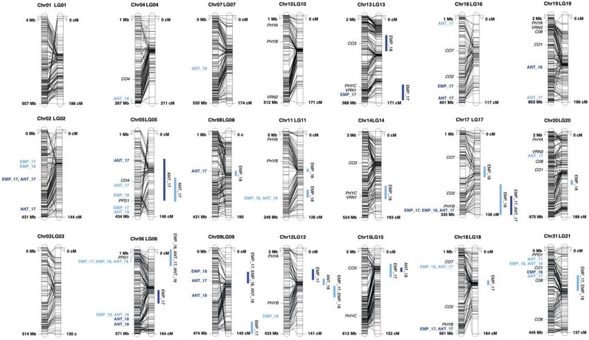
Figure 1 Distribution of progeny emmeans within the 10 IWG NAM families for emergence percent (A) and anthesis score (B) at St. Paul (STP) and the
Land Institute (TLI) in 2017 and 2018. Black horizontal lines within boxplots are progeny means. Horizontal gray dotted line indicates common parent
mean and colored dots indicate parent means. Families are ordered based on their ranking for STP 2017.
distribution of individuals, with the common parent in the cen-
ter, and progeny distributed approximately mid-way between
parents, demonstrated the expected relationship (either half- or
full-sibs) between individuals in the population.
Consensus linkage map creation
After filtering for MAF and missing data within families, an aver-
age of 3,003 markers per family (average 143 per LG) were used
for initial linkage mapping analysis. Across families, 40% (range:
36%–43%) of markers displayed significant segregation distortion
at a ¼ 0.1, and were excluded from the map making step
(Supplementary Figure S6). A greater proportion of the hkxhk
type markers (average 71%) exhibited distortion, followed by
lmxll (28%), and nnxnp (24%). In the case of LG 18, there was an
insufficient number of undistorted lmxll (common parent,
Figure 2 Principal components (PC) analysis of the intermediate
wheatgrass nested association mapping population families, where large WGN59) markers to contribute to the map and thus the map for
dots indicate parents, small dots indicate progeny and colors indicate LG 18 only includes nnxnp markers. The final map length aver-
family identity. Axis labels include percent variance explained for the aged 161 cM per LG with a total length of 3,385 cM (Haldane’s
two PCs. mapping units) and a density of one marker per 0.93 cM
(Figure 3). Pearson correlation was used to assess the quality of
Marker data and SNP filtering the map order using markers in common with the consensus ge-
netic map (Kantarski et al. 2016) and 17 LGs were above r ¼ 0.95,
Initial SNP marker count was 444,023 which was reduced to 8,003
after filtering. Two genets were removed because they had with four having lower correlations (Supplementary Figure S7).
Markers that exhibited distortion in one family, but were in-
greater than 70% missing marker data. The common parent had
cluded in map making in another, were allowed to phase in the
a high propensity for self-pollination with a rate of 8.3% (range of
creation of the .loc files for use in MapQTL. There were approxi-
1.5%–15.9%, depending on the family), while the donor parents
mately 1,652 markers per family in common between the consen-
averaged 2.9% (range of 0%–11.4%, depending on the family). A
sus and the final NAM map with an average of 78 per LG
total of 74 individuals were removed from the final analysis be-
(Supplementary Figure S8). To implement the TWPT, hkxhk
cause they were identified as progeny derived from self-
markers were excluded which reduced this number to an average
pollination or unintended outcrosses. Final family size on aver-
of 994 markers per family and 47 markers per LG.
age was 117 individuals. Imputation accuracy for LinkImpute
was 95.3%. Linkage disequilibrium, as defined by r2 ¼ 0.2, varied
across linkage groups with a range of 14.5 cM for LG 20, and 53.5 Genome wide association
cM for LG 18 with a median of 21.08 cM (Supplementary Figure Nineteen and twenty-six marker-trait associations were detected
S5). The first two principal components of the genotype matrix for the emergence percent and anthesis score respectively across
explained 22.2% and 15.5% of the variation (Figure 2). The the four environments using GWAS (Figure 3; Table 2). Seven8 | G3, 2021, Vol. 11, No. 3
Downloaded from https://academic.oup.com/g3journal/article/11/3/jkab025/6124305 by guest on 12 December 2021
Figure 3 For each chromosome, the physical map (unpublished, access provided by the Thinopyrum intermedium Genome Sequencing Consortium) is on
the left, and linkage maps developed in the present study are on the right. Markers that were used in both mapping approaches are connected with a
line. Physical distances in megabase pairs (mbp) and genetic distances in centimorgans (cM) are normalized to comparable lengths. Included on the
physical map (left), are the significant markers from GWAS and possible candidate orthologous genes (black italic). Included on the linkage map (right)
are the 2-LOD drop off intervals for the combined analysis across populations (bars indicate interval length), for STP (light blue) and TLI (dark blue) for
emergence percent (EMP) and anthesis (ANT) followed by the years (17 and 18 for 2017 and 2018) in which the marker interval was detected.
were significant in two trait environment combinations, and two 2016). Importantly, we determined that the common parent,
in three environment trait combinations. Markers generally WGN59, was derived from a mating of at least half-siblings (male
explained a small percent of the variation for a trait, for a median parents are unknown), leading to a minimum inbreeding coeffi-
of 1.7 and 1.9 for emergence and anthesis, respectively. Allele cient for that individual of F 1=8. Parent WGN26 is a half-sibling
effects corresponded to a median absolute difference of 6.5% to WGN59 (coefficient of coancestry, fWGN26, WGN59 1=8). Parents
spike emerged, or a 0.35 fraction of a growth stage. Most QTL WGN36 and WGN38 were full siblings, and along with WGN15,
were detected on chromosomes 5, 2, 6, 21, 9, and 16. Most QTL they share a common grandmother (C3-3471) with WGN59
were detected at STP 2018 (15) and fewest were detected at TLI (fWGN36, WGN59 ¼ fWGN38, WGN59 ¼ fWGN15, WGN59 1/16). Parent C3-
2018 (7). 3471 was the first nonshattering, 90% free-threshing plant de-
rived from The Land Institute’s breeding program and has been
QTL linkage mapping used in numerous crosses in the UMN program and in the crea-
In the combined analysis, 24 and 8 QTL intervals detected for tion of the consensus genetic map (Kantarski et al. 2016). We also
emergence percent and anthesis score, respectively. Of these, five identified interrelatedness among six donor parents that are
were identified in more than one trait or environment (Figure 3; half-sibs, sharing either a mother or father in common, includ-
Table 3), and the majority (62.5%) were identified as segregating ing: WGN39 and WGN63, WGN07 and WGN46, WGN45 and
in the donor parent. In the individual family analyses, the most WGN55.
QTL were detected in families 15 (10), 26 (10), and 36 (10). A QTL
detected in the combined analysis typically overlapped anywhere
between zero and five significant within-family QTL (Table 3). Discussion
Allele effects and variance explained are only calculated in the IWG is currently undergoing domestication as a perennial grain
within family analyses. The median variance explained for a QTL crop for human consumption. Selection targets for this crop are
was 14.8% (range 8.6%–73.3%). The most QTL were found on LG 6 numerous and the understanding of the genetic control of impor-
(12 in unique analysis by trait by environment combinations), LG tant traits remains relatively unknown. NAM as a method for
17 (11), and LG 12 (10). marker-trait dissection has proven useful in other crops but has
not been tested before in a species with this mating system, one
Pedigree relationships that is self-incompatible and requires the use of F1 progeny. We
Using pedigree records and historical genotype data from the examined a 10-family F1 NAM of IWG developed with phenotypi-
breeding program, we determined multiple shared relationships cally diverse parents from Cycle 2 of the University of Minnesota
between the NAM parents, which were initially selected based on breeding program. Considering the importance of variation in
phenotype alone (Supplementary Figures S9 and S10; Zhang et al. flowering time for optimizing yield and performance in newK. R. Altendorf et al. | 9
Table 2 Results from genomewide association mapping results for all environments organized by trait and environment (top row). Instances in which the QTL
was not detected in the present environment are indicated by missing values (“—").
STP 2017 STP 2018 TLI 2017 TLI 2018
a b c e f g
Trait SNP Alleles MAF Segregating 2log10(p) Effect PVE log10(p) Effect PVE log10(p) Effect PVE log10(p) Effect PVE
Familiesd
Emergence Chr02_163115345 T/C 0.11 15, 63 3.93 –0.07 3.65 — — — — — — — — —
Percent Chr02_178305818 T/C 0.16 26, 38, 39, 45, 55, 63 — — — 3.66 0.05 0.84 — — — — — —
Chr02_245307556h C/T 0.02 38 — — — — — — 5.2 0.18 1.44 — — —
Chr05_327412330 A/G 0.05 36, 39 — — — 3.87 –0.07 1.44 — — — — — —
Chr05_392431630 C/G 0.05 39, 63 3.68 –0.07 1.63 — — — — — — — — —
Chr06_27073072h T/C 0.44 All 4.27 0.03 2.34 9.53 0.06 3.27 — — — — — —
Chr06_445976596h G/T 0.34 07, 15, 38, 45, 46, 55 — — — 7.1 –0.06 1.05 — — — — — —
Chr09_131144770 A/G 0.26 07, 36, 39, 45, 46, 63 — — — — — — — — — 4.36 –0.06 2.41
Chr11_193858632h G/A 0.05 39, 55 — — — 3.87 –0.07 0.58 — — — — — —
Downloaded from https://academic.oup.com/g3journal/article/11/3/jkab025/6124305 by guest on 12 December 2021
Chr12_347517636 A/G 0.13 26, 39, 45, 55, 63 — — — 3.75 0.05 0.91 — — — — — —
Chr13_347308338 C/T 0.13 15, 38, 39 — — — — — — 3.66 –0.08 0.82 — — —
Chr16_326253169 G/C 0.47 All — — — — — — 3.82 –0.05 1.67 — — —
Chr17_317374690h G/C 0.36 All — — — — — — 4.25 –0.05 2 3.81 –0.04 2.01
Chr18_112460873h G/A 0.05 36, 38 — — — 4.79 –0.08 1.7 — — — — — —
Chr18_550223545h G/C 0.16 07, 36, 38, 39, 45, 55 — — — — — — 5.17 0.07 1.76 — — —
Chr21_75063069h T/A 0.19 07, 36, 38, 46, 63 — — — 3.7 –0.05 2.46 — — — — — —
Chr21_121306193 C/T 0.02 07, 15 — — — — — — — — — 4 0.1 0.78
Anthesis Chr02_245307556h C/T 0.02 38 — — — — — — 5.47 0.79 2.82 — — —
Score Chr02_391596222 G/A 0.15 07, 38, 45, 46 — — — — — — 3.93 0.3 2.03 — — —
Chr04_266676626 T/C 0.15 26, 39, 45, 46, 55, 63 — — — 3.81 0.26 1.53 — — — — — —
Chr05_152472752 T/C 0.12 45, 46, 55 — — — — — — 4.48 –0.35 3.15 — — —
Chr05_269372528 C/T 0.02 26 5.96 0.75 2.91 — — — — — — — — —
Chr05_426524999 G/C 0.25 15, 26, 36, 38, 39, 45, 46 — — — 4.11 –0.25 1.77 — — — — — —
Chr06_27073072h T/C 0.44 All — — — 10.02 0.32 4.08 — — — — — —
Chr06_445976596h G/T 0.34 07, 15, 38, 45, 46, 55 — — — 6.37 –0.32 0.76 — — — — — —
Chr06_470381731 G/T 0.45 All — — — — — — — — — 5.58 0.28 2.07
Chr06_507506304 C/T 0.40 All — — — — — — — — — 3.65 0.28 0.54
Chr07_315344031 C/T 0.05 39, 55 — — — 4.25 –0.44 0.08 — — — — — —
Chr08_202486528 T/C 0.05 07, 46 — — — — — — 4.12 –0.49 0.93 — — —
Chr09_183303350 C/T 0.02 46 — — — — — — 4.48 0.65 0.99 — — —
Chr09_265159585 C/T 0.03 07 — — — — — — — — — 3.67 0.72 0
Chr11_193858632h G/A 0.04 39, 55 — — — 4.94 –0.46 0.52 — — — — — —
Chr16_34501928 T/C 0.05 26, 55 3.76 0.36 0.4 — — — — — — — — —
Chr16_397627839 G/A 0.39 All — — — — — — 3.89 0.2 2.37 — — —
Chr17_317374690h G/C 0.36 All — — — — — — 5.32 –0.24 1.9 — — —
Chr18_112460873h G/A 0.05 36, 38 4.05 –0.41 1.78 — — — — — — — — —
Chr18_550223545h G/C 0.16 07, 36, 38, 39, 45, 55 — — — — — — 4.85 0.27 1.95 — — —
Chr19_484430789 T/C 0.03 07 — — — — — — — — — 4.27 0.78 1.85
Chr19_762292265 C/T 0.07 15, 39, 45 4.78 0.38 1.98 — — — — — — — — —
Chr20_193202832 C/T 0.11 15, 45, 55 3.73 0.35 0.5 — — — — — — — — —
Chr21_33179355 G/A 0.12 26, 36, 38, 55, 63 3.98 –0.28 2.52 — — — — — — — — —
Chr21_75063069h T/A 0.19 07, 36, 38, 46, 63 — — — 4.76 –0.34 3.06 — — — — — —
Chr21_131911561 G/C 0.3 07, 36, 38, 39 4.36 0.33 3.8 — — — — — — — — —
a
SNP, single nucleotide polymorphism, including chromosome number followed by position in base pairs.
b
Reference and alternate alleles.
c
Minor allele frequency within the entire 10-family NAM population.
d
NAM families in which the allele segregates above a frequency of 0.05.
e
Level of significance.
f
Allele effect in trait units, associated with the alternate allele.
g
PVE, percent variance explained by the QTL.
h
Indicates a SNP detected in both traits.
environments, we sought to increase our understanding of the supported by the QTL linkage mapping results, which was signifi-
genetic control of flowering time in IWG and determine the utility cant in three analyses in STP. In GWAS, the allele segregated in
of this population for genetic mapping. all ten families, and explained on average 3.23% of the variation
Two methods were used to detect QTL for flowering time, (Table 2). In linkage mapping, this region was detected in the
GWAS and two-way pseudo testcross linkage mapping using both combined analysis and in families 15 and 55 where it explained
a combined and within population analysis and a genetic map on average 19% of the variation, suggesting that this marker may
created specifically for the NAM. In most cases, regions with have family specific effects (Table 3). A TLI-specific QTL on chro-
many GWAS QTL coincided with significant linkage mapping mosome 17 was detected in GWAS (Chr17_317374690) in three of
intervals that were consistent across multiple trait and environ- four TLI analyses and was supported by an overlapping QTL in-
ment combinations (Figure 3). Furthermore, these regions, specif- terval (peaking around an average of 127 cM) that was detected
ically on chromosomes 6, 17, 14, 5, and 21, were in supported by in two of four analyses at TLI and one at STP. The GWAS QTL was
BLAST hits and corresponding gene models to orthologous barley within 66 mpb and 57 kb from significant BLAST hits for the
flowering time genes. On chromosome 6, GWAS marker orthologous genes Constans 2 and PHYB, respectively (Griffiths
Chr06_27073072, which was detected in in both STP years for } cs et al. 2006). Though only detected using linkage
et al. 2003; Szu
emergence percent and for anthesis in STP 2018 is 23.9 kb away mapping in emergence percent at STP in 2018, a QTL interval on
from a significant BLAST hit and corresponding gene model for LG 14 aligned closely with a hit for PHYC and VRN1 (Fu et al. 2005;
the well-characterized Ppd-H1 gene in barley that delays flower- Nishida et al. 2013). On chromosome 5, we detected, across both
ing time (Turner et al. 2005; Figure 3). This QTL region is further approaches and in multiple environments, QTL that aligned nearYou can also read