Network Options Assessment for Interconnectors - National Grid ESO
←
→
Page content transcription
If your browser does not render page correctly, please read the page content below

Network Options Assessment
for Interconnectors
May 2019 | Network Options Assessment Report Methodology   36
Electricity System Operator                                                                         May 2019

Overview
3.1     This chapter provides an overview of the aims of the NOA with respect to interconnectors and
        details the methodology which the ESO will adopt for the analysis and publication within the
        fifth NOA report (to be published by 31st January 2020).
3.2     We have continued to develop the NOA for Interconnector methodology. This chapter
        represents our latest thoughts. We will continue to actively consult, listen and respond to
        feedback from our customers and stakeholders on this methodology. This will enable us to
        revise and improve the methodology, resulting in a NOA for Interconnectors analysis that is of
        increasing value for our stakeholders.
3.3     For reference, below is a summary of the key features and developments of the previous
        NOA for Interconnector methodologies.

 NOAIC 1 (2015/16)            NOAIC 2 (2016/17)            NOAIC 3 (2017/18)             NOAIC 4 (2018/19)

 - Modelled through ELSI      - Modelled through Pan       (As per NOAIC 2 plus…)        (As per NOAIC 3 plus…)
 - GB consumer surplus          European Market Model      - Use of FES 2017             - Use of FES 2018
   only                         (BID3)                       backgrounds                   backgrounds, including
 - Price data procured from   - SEW as sum of              - Used optimized network        European FES
   industry                     producer and consumer        found through NOA3 as       - Provide a range of
 - Only considered existing     surplus as well as           baseline                      solutions by not
   interconnectors and          interconnector revenue     - Combination of                undertaking least worst
   those applied through      - Consideration of benefit     interconnectors and           regret
   C&F                          of additional capacity       potential reinforcement     - Analysis of the impact of
 - Copper plate model with    - Copper plate model         - Single optimal path           interconnectors on
   no transmission              with no transmission         generated through a least     system operability
   constraints                  constraints                  worst regret approach

Network Options Assessment Report Methodology – Draft 5.0 – 09/05/2019                         Page 37 of 117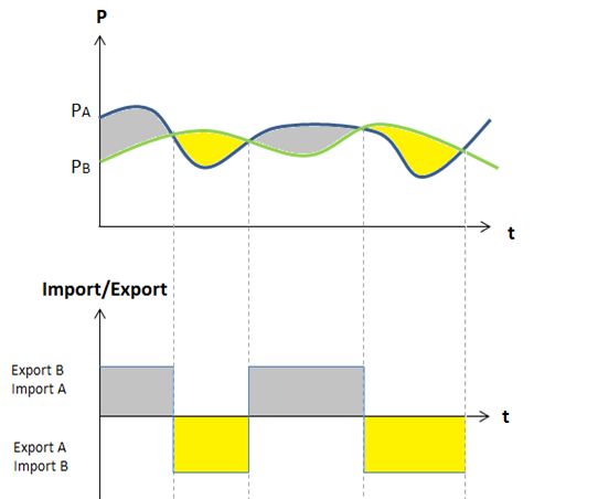
Electricity System Operator                                                                    May 2019

Structure of this section
3.4     This section consists of the thirteen sub-sections listed below:
        •   Key changes to 2019/20 methodology - A summary of the major changes made to the
            NOA for Interconnector methodology for 2019/20.
        •   Key similarities to the 2018/19 methodology - A summary of which areas of the
            methodology have remained the same from 2018/19 to 2019/20.
        •   Factors for the assessment of future interconnection - A justification of the factors to
            be considered in determining whether additional capacity would be beneficial.
        •   Cost estimation for interconnection capacity – The costs associated with an
            interconnector and how these will be calculated.
        •   Cost estimation for network reinforcement – The costs associated with network
            reinforcements and how these will be calculated.
        •   Components of welfare benefits of interconnection – This sub-section outlines the
            concept of Socio-Economic Welfare in relation to interconnection and the components of
            the calculation.
        •   Constraint cost implications – An outline of how interconnectors could impact the
            operational costs on the network.
        •   Ancillary Services – A description of the system needs for operability, and how
            interconnection’s impact on these will be assessed.
        •   BID3 model – A description of the ESO’s current market modelling capabilities
        •   Options included within the assessment – A listing of the options that will be assessed
            within the modelling.
        •   Interconnection assessment methodology – A description of the method by which the
            ESO proposes to meet the aims of the NOA in relation to optimal interconnection
            capacity.
        •   Further Output – Additional results that may be of benefit to stakeholders.
        •   Process Output – How the NOA IC output will be delivered.

Key changes for 2019/20 methodology
3.5     This year we will continue to improve the NOA for Interconnectors analysis by acting on
        feedback from our stakeholders.
3.6     We will refocus on providing additional value from the main iterative analysis on social
        economic welfare, capital costs and constraint costs, by drawing greater insights from the use
        of the European FES, which improve the quality and range of interconnector modelling that
        drives the NOA IC analysis.
3.7     We will investigate revising the interconnector baseline level: whereby all current projects and
        those with regulatory certainty will still be included, but add an “uncertainty factor” to reduce
        the baseline level of interconnection.
3.8     We will use the NOA IC as a signpost to other system operability work being undertaken
        within the System Operability Framework, rather than attempt to undertake an analysis of the
        impact of interconnectors on system operability within the NOA IC analysis.

Key similarities to 2018/19 methodology
3.9     We will continue to take into consideration the locational impacts on the GB transmission
        network in addition to the welfare and capital cost implications.
3.10    We will continue focus on Social Economic Welfare, capital costs and reinforcement costs.
3.11    We will use the output from the 2019/20 NOA as the baseline network reinforcement
        assumptions for the NOA IC analysis: this provides greater consistency between the NOA
        and NOA IC analysis which we believe is of added value to our stakeholders.
3.12    We intend to use essentially the same iterative method used last year. The studies will involve
        a step-by-step process, where the market is modelled with a base level of interconnection,
        including current interconnection levels and projects with regulatory certainty. Four separate

Network Options Assessment Report Methodology – Draft 5.0 – 09/05/2019                     Page 38 of 117
Electricity System Operator                                                                     May 2019

        solutions will be created and hence a range for the optimal level of interconnection, as in NOA
        IC 2018/19, which stakeholders felt was more realistic and useful.
3.13    We will continue to calculate Social Economic Welfare for all EU countries as well as for GB
        and the connecting country. We will investigate whether there is any benefit in calculating the
        optimal path based on the Social Economic Welfare of GB and the connecting country only.
3.14    We will continue to highlight the impact of interconnection on carbon costs and renewable
        energy curtailment.
3.15    We will provide a similar level of detail to that provided in NOA IC 2018/19, but continue to
        provide greater insight and explanation into what is driving the results and also improve
        graphical representation of results.
3.16    We will continue to develop NOA IC based on stakeholder recommendations

Costs included within the methodology scope
3.17    There are multiple factors which could be considered when evaluating interconnector
        projects. The foremost are social economic welfare, capital costs and impact on constraint
        costs. Constraint costs refer to GB network congestion costs borne by GB consumers as a
        result of interconnection.
3.18    SEW, CAPEX and Attributable Constraint Costs (ACC) are the most significant criteria for
        identifying the optimal level of interconnection. Therefore, these factors will be used in the
        analysis to determine the economically optimal level of interconnection.
3.19    Two further factors that will be analysed and have some accompanying commentary in the
        NOA report are changes in carbon emissions and use of Renewable Energy Sources (RES).
        These indicators are intended to aid understanding of interconnection’s potential impact to
        meeting GB’s climate change goals. They will not be used to optimise the interconnection
        presented. This is due to the complexity of combining Carbon/RES estimates with welfare and
        cost, especially where modelled welfare is already influenced by such factors through RES
        incentives and the European Trading System capping carbon emissions.
3.20    Carbon costs: modelling facilities allow for the extraction of total carbon emissions resulting
        from particular market states under different scenarios, thus the carbon savings or increases
        associated with various levels of interconnection can be presented with commentary.
3.21    RES integration: modelling facilities allow for the investigation of impact of interconnection
        on renewable generation. This can be reviewed through investigating the reduction or
        increase in renewable generation curtailment driven by the optimal level of interconnection
        being in place in future years, rather than the currently forecast level.

Network Options Assessment Report Methodology – Draft 5.0 – 09/05/2019                      Page 39 of 117
Electricity System Operator                                                                           May 2019

Costs outside the methodology scope
3.22     There are further benefits and costs that could be considered, which are briefly outlined
         below; they are outside the scope of this methodology:
3.23     Operational costs: Various costs associated with the day-to-day operation of the
         interconnector, and the maintenance of its components, are omitted from the analysis. This is
         driven by the complexity of defining these costs, per market. There is a high correlation
         between capital spend (which is included) and these operational costs. Moreover, there is
         unlikely to be a substantial variation in the ‘standard’ operational costs per European market
         under consideration, meaning it is equitable to remove them from consideration for all
         markets. One may argue that the operational costs may cause the end of the optimal path to
         be reached sooner however a decision has been made to omit this factor from the analysis
         due to the insignificance in relation to SEW over 25 years.
3.24     Environmental/social costs: In any large scale construction project, the local environment
         may potentially suffer damage. This affects local stakeholders, as well as disruption
         associated with the construction (traffic, noise etc.). The severity varies with the site chosen
         and the construction methods used. These are not considered here as they are more relevant
         to the choice of sites for individual projects.
3.25     Social benefits: Depending upon the procurement for the construction, the project may offer
         a boom to the local economy. This again is a project specific benefit, so is not estimated in
         this work.
3.26     Ancillary Service costs: We will not attempt to model the potential impact of interconnectors
         on services which support system operability. Initial feedback on the system operability
         analysis undertaken for NOA IC 2018/19 was mixed. The results were complex and difficult to
         draw high level conclusions from. Some stakeholders felt the analysis placed an inappropriate
         focus on the benefit or disbenefit of interconnectors on system operability, and that a wider
         lens would be more appropriate. There were also concerns with the robustness of analysis so
         far into the future.
3.27     A more detailed analysis of system operability as part of NOA for Interconnectors does not fit
         well with the high-level market signal approach of other NOA for Interconnectors market
         analysis work. In addition, the time available for the NOA for interconnectors modelling, which
         can only commence after the NOA reinforcement recommendations are available and must
         be complete before the end of January, makes this infeasible.
3.28     We believe a more appropriate solution is to undertake this type of analysis as part of the
         System Operability Framework which takes a holistic view of the changing energy landscape
         to assess the future operation of Britain's electricity networks. Interconnectors may be one of
         a range of potential service providers or may be one of a range of assets that may result in
         system operability issues. The NOA for Interconnectors analysis can be used as a means of
         highlighting this work.

Cost estimation for interconnection capacity
3.29     The cost of building interconnection capacity varies significantly between different projects -
         key drivers are convertor technology, cable length and capacity of cable. Estimating costs for
         generic interconnectors between European markets and GB is therefore challenging. An
         exercise of a similar nature has been undertaken by various industry bodies to allow the
         generation of ‘Standard Costs’. These are generic values that can be applied to estimate the
         cost of generic projects. A report by ACER15 provides sufficient granularity to differentiate
         between standard costs of connection to different markets. There are three elements to the
         capital costs; subsea cable, onshore connection costs and wider reinforcement costs. We will
         continue to review and investigate alternative robust sources for generic interconnector cost
         estimates.

15
 http://www.acer.europa.eu/Official_documents/Acts_of_the_Agency/Publication/UIC%20Report%20%20-
%20Electricity%20infrastructure.pdf

Network Options Assessment Report Methodology – Draft 5.0 – 09/05/2019                             Page 40 of 117
Electricity System Operator                                                                                 May 2019

3.30     Subsea cable costs will be identified by estimating the furthest and shortest realistic subsea
         cable length and taking the average distance for each market to GB zone permutation.
         Suitable substations have been identified using the ENTESO-E Transmission System Map.
         For each market and GB zone (as defined in paragraph 3.31), only logical substations which
         are neighbouring or have sufficient infrastructure will be reviewed in the study of route length.
         The length of the cable will vary with the GB zone it is connecting to and the measurements
         will be taken between these to the nearest 5km and are shown in the following table.
Table 3. 1 Route distances

 Country                GB Zone       Distance (Km)
 Norway                       1                    705
 Norway                           2                     795
 France                           5                     175
 France                           6                     100
 Netherlands                      4                     215
 Netherlands                      6                     210
 Denmark                          4                     620
 Denmark                          7                     660
 Ireland                          2                     220
 Ireland                          3                     220
 Germany                          4                     520
 Germany                          7                     590
 Belgium                          4                     185
 Belgium                          6                     140
 Spain                            5                     810

3.31     Onshore connection costs will be excluded as the interconnector study cases are zone
         specific but not substation specific.
3.32     Wider reinforcement costs will be included in capital costs for options where applicable.
3.33     The convertor station assumed value is drawn from an averaging of known HVDC projects
         performed by ACER. The ACER cost estimates are shown in the table below (these costs
         include the cost of installation):
Table 3. 2 Standard costs

 Total cost per route           Rating                             Mean
 length (km)                                                       (€, 2014)

 DC cables16                    250-500kV                          757,621

16
  The DC cable cost provided is for a 500MW cable. An assumption has been made that for a 1000MW interconnector the cost
per km will be double.

Network Options Assessment Report Methodology – Draft 5.0 – 09/05/2019                                  Page 41 of 117
Electricity System Operator May 2019
OHL17 380-400kV (2 circuits) 1,060,919
Underground cables21 380-400kV (2 circuits) 4,905,681
Total cost per rating (MVA) Mean
(€, 2014)
HVDC convertor station 87,173
3.34 At the start of the analysis, the suitable rate of conversion from 2014 euros to present day
sterling will be drawn from a credible source available to the ESO (Bloomberg). The table can
then be used to generate a generic cost for a given increase in capacity for each market. As
connection can occur across a range of years, discounting is employed to standardise each
cost in Present Value. This is done with the Social Time Preference Rate (STPR) of 3.5%.
Additionally, the cost of capital is taken account of through the use of a Weighted Average
Cost of Capital (WACC) of 6.8% for interconnectors, drawn from a publicly available Grant
Thornton report.18
Cost estimation for network reinforcements
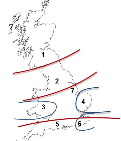
3.35 The network has been divided into seven high level zones which have been determined by
areas of significant constraints on the network or areas of high interconnection as illustrated in
Figure 3. 1.
a
b
c
f d
e
Figure 3. 1 Illustration of Network Zones
3.36 The baseline boundary capabilities will be determined by using the outputs from the main
NOA 2019/20 analysis. Additional boundaries, and hence zones may be added if their
addition may increase the value of the analysis.
17
The rating on the figures above is sufficient to accommodate an additional 2000MW of interconnection. Therefore, the figures
will be adjusted to incur 70% of the total cost for the first 1000MW of capacity required and 30% for the second 1000MW of
reinforcement capacity on the same boundary.
18
https://www.ofgem.gov.uk/ofgem-publications/51476/grant-thornton-interest-during-construction-offshore-transmission-
assets.pdf
Network Options Assessment Report Methodology – Draft 5.0 – 09/05/2019 Page 42 of 117Electricity System Operator May 2019
3.37 Generic reinforcements will be created for each boundary. These will be based on where
there are high levels of congestion on the network and an indication of the level of
reinforcements required.
Components of welfare benefits of Interconnectors
Introduction
3.38 This section outlines the definition of Social Economic Welfare. The purpose of this section is
to give the theoretical background of assessing the impact of connected importing and
exporting markets on consumers, producers and interconnectors triggered by another
interconnector.
Social and Economic Welfare
3.39 Social and Economic Welfare (SEW) is a common indicator used in cost-benefit analysis of
projects of public interest. It captures the overall benefit, in monetary terms, to society from a
given course of action. It is important to understand it is an aggregate of different parties’
benefits - so some groups within society may lose money as a result of the option taken. The
society considered may be a single nation, GB, or the wider European society, in which case
the benefits to European consumers and producers would be a part of the calculation. For the
case of GB interconnectors, it is most informative to show both GB and the connected
market’s SEW values, and the components which make up each.
3.40 SEW benefits of an interconnector includes the following three components:
a) Consumer surplus, derived as an impact of market prices seen by the electricity consumers
b) Producer surplus, derived as the impact of market prices seen by the electricity producers
c) Interconnector revenue or congestion rents, derived as the impact on revenues of
interconnectors between different markets.
3.41 Interconnectors could help to provide ancillary services (including black start capability,
frequency response or reserve response), facilitate deployment of renewables, reduction in
carbon emissions and displace network reinforcements. Interconnectors also provide benefits
of being connected to more networks giving access to a more diverse range of generation
which could lead to reduction in carbon emissions. Such benefits will not be a part of the main
NOA IC assessment, as discussed in the previous section.
Effects on Interconnected markets
3.42 Power flow between two connected markets is driven by price differentials. Figure 3. 2 shows
the effects of such price differentials for two markets, A and B with variable prices over time.
When the price is higher in market A, power will be transferred from B to A. When the price in
A is lower than B power will be transferred from A to B.
Network Options Assessment Report Methodology – Draft 5.0 – 09/05/2019 Page 43 of 117Electricity System Operator May 2019
Figure 3. 2 Price difference as import and export driver
3.43 Figure 3. 3 shows the impact of an interconnector (+IC) linking two markets on consumer
(Demand D) and producer (Supply S) costs. When two competitive markets with different
price profiles are interconnected, price arbitrage drives power flow from the low price market
(B) to the high price market (A). Consumers in market A are likely to gain (a + b) as they
benefit from access to cheaper power. Consumers in market B are likely to lose (d).
Generators in market A must now also compete with generators in B and are likely to be
forced by competitive pressures to reduce their costs. This may lead to a reduction in their
profits (a). Producers in market B are likely to gain (d + e). Interconnector revenue (c) is
derived from the remaining price difference.
Figure 3. 3 Consumer and Producer Surplus of connected markets
3.44 With greater interconnection, the price difference between markets will decrease thus the
revenue of the interconnector will be reduced as well. This phenomenon is known as
‘cannibalisation’. There is an optimal level of interconnection between any two markets
because price differential reduces as capacity increases, i.e. area c in Figure 3. 3 shrinks.
3.45 Forecasts of all components of SEW benefits will be key drivers to ascertain the optimum
level of interconnection between GB and other European states. The outputs of this process
will include monetised impacts on consumers, producers and considered interconnectors.
Network Options Assessment Report Methodology – Draft 5.0 – 09/05/2019 Page 44 of 117Electricity System Operator May 2019
3.46 The Global SEW is the sum of the welfare of 5 parties (GB consumers, Europe consumers,
GB producers, Europe producers and Interconnector owners). The British SEW is the sum of
the welfare of all British parties. Using the ownership structure of existing GB interconnectors,
assuming 50% of interconnector owner welfare remains in the GB economy is plausible.
3.47 Where the market is modelled with and without some additional interconnection capacity
added, SEW is modelled in each year of a generic asset’s lifetime (25 years is the standard
assumption used here). As connection can occur across a range of years, discounting is
employed to standardise each year’s benefit in Present Value, also allowing comparison with
the discounted capital spend. This is done with the Social Time Preference Rate of 3.5%.
Constraint cost implications of interconnection
3.48 The impact on constraint costs is dependent on the location of the interconnector on the GB
network and the level of onshore reinforcement built to accommodate the interconnector.
Further detail regarding optimal locations to connect will be output based upon the constraint
costs calculated on the network with the interconnectors under consideration.
3.49 Constraint costs are incurred on the network when power that is economically “in merit” is
limited from outputting due to network restrictions. In this event, the ESO will incur balancing
mechanism costs to turn down the generation which is not able to output and offer on
generation elsewhere on the system to alleviate the constraint.
3.50 The output of the ETYS and NOA reports provides information on the current state and
ongoing developments of the onshore network. This will be used to provide a general picture
of the optimal network areas for accommodating interconnectors from certain countries. This
will be based on constraint costs attributable to the interconnector under review. ETYS and
NOA quantify the boundary limitations and present recommended options for reinforcement of
the grid. This is intrinsically linked to the increasing presence of interconnection in the UK
which can cause further strain on boundaries and potentially trigger investment in further
reinforcements if the NOA process determines that to be the most economic and efficient
course of action.
BID3 model
3.51 BID3 is the tool which will be used to perform the NOA IC 2019/20 and employed by the ESO
to carry out a range of economic analysis.
3.52 BID3 is a Pan European Market Model created by Pöyry Management Consultants. BID3 will
be used by National Grid to forecast the Socio-Economic Welfare (SEW) and the Attributable
Constraint Costs (ACC).
3.53 A comprehensive guide to how National Grid uses BID3 for calculating constraints is available
on our website19. It is an economic dispatch model which can simulate all ENTESO-E power
markets simultaneously from the bottom up i.e. it can model individual power stations for
example. It includes demand, supply and infrastructure and balances supply and demand on
an hourly basis. BID3 models the hourly generation of power stations on the system, taking
into account fuel prices, historical weather patterns, socio-economic welfare and operational
constraints.
3.54 The GB electricity system in BID3 is represented by a series of zones that are separated by
boundaries. Generators are allocated to their relevant zone based on where they are located
on the network, and then the appropriate demand is allocated to that zone. The boundaries,
which represent the actual transmission circuits facilitating the zonal connectivity, have a
maximum capability that restricts the amount of power which can be securely transferred to
across them.
3.55 The socio-economic welfare is calculated by summing the producer surplus, consumer
surplus and interconnector revenue. The consumer surplus is the difference between the
19
https://www.nationalgrid.com/sites/default/files/documents/Long-
term%20Market%20and%20Network%20Constraint%20Modelling.pdf
Network Options Assessment Report Methodology – Draft 5.0 – 09/05/2019 Page 45 of 117Electricity System Operator May 2019
value of lost load and the wholesale price. The producer surplus is calculated and summed
per plant based upon their Short Run Marginal Cost and the wholesale price.
3.56 Case collections are used for hourly generation and demand profiles as well as solar and
wind profiles. An extensive study has identified the average historic year in terms of
Generation, Demand, Wind output, Solar Output, interconnector flows and hydrological year.
This is an approved approach but has limitations and could potentially undervalue countries
with a high level of renewable generation such as Nordic countries with significant levels of
hydro power.
Options included in the assessment
3.57 As there are infinite combinations of markets and reinforcements, applying engineering
judgement, the number of options has been reduced to 29 credible study cases. These 29
study cases will be assessed in all iterations across all four scenarios.
3.58 The options which will be assessed are included in Table 3. 3 below. The boundary
reinforcements and zones refer to Figure 3. 1.
Table 3. 3 Options to be considered in the analysis
Market and Zone Boundary Market and Zone Boundary
Reinforcements Reinforcements
Belgium Zone 4 c Ireland Zone 2 b
Belgium Zone 4 None Ireland Zone 2 None
Belgium Zone 6 None Ireland Zone 3 None
Belgium Zone 6 d+e Netherlands Zone 4 c
Denmark Zone 4 c Netherlands Zone 4 None
Denmark Zone 4 None Netherlands Zone 6 None
Denmark Zone 7 None Netherlands Zone 6 d+e
France Zone 5 None Norway Zone 1 a+b
France Zone 5 d Norway Zone 1 None
France Zone 6 None Norway Zone 2 b
France Zone 6 d+e Norway Zone 2 None
France Zone 6 d Spain Zone 5 None
Germany Zone 4 c Spain Zone 5 d
Germany Zone 4 None
Germany Zone 4 f
Germany Zone 7 None
Network Options Assessment Report Methodology – Draft 5.0 – 09/05/2019 Page 46 of 117Electricity System Operator May 2019
Interconnection Assessment Methodology
Optimisation of GB-Europe Interconnection Process
Run the model with
each interconnector in
sequentially for each
FES
Update each FES path Assess the net benefit
with the relevant optimal of each potential
solution interconnector study
case for each FES
Figure 3. 4 Process summary
3.59 The optimisation of future interconnection capacities is a multivariable search, maximising the
SEW less CAPEX less Attributable Constraint Costs (ACC) value. The decision variables are
the total MW capacities (the sum of all interconnector transfer capacities) between GB and 8
adjacent markets, for both importing and exporting. These markets are national electricity
markets- there is some level of coupling between many of them, however price areas (areas
with the same electricity price throughout) generally align with nations. Where some nations
have multiple price areas, such as Norway, interconnector projects will be assumed to be in
the coastal price area deemed most likely for interconnection to the UK. The countries in
question are: Norway; Denmark; Germany; The Netherlands; Belgium; France; Spain; and
Ireland (which includes the Republic of Ireland and Northern Ireland). For each country’s
additional interconnector capacity, there will be a small number of zones and reinforcement
combinations studied. The number of variables makes an exhaustive search within a useful
timeframe infeasible - a search strategy must therefore be defined.
3.60 Due to the unique properties of the Icelandic market, any interconnection to Iceland which
appears in the Future Energy Scenarios (FES) will remain in the background. Further
Icelandic interconnection will be removed from the iterative process.
3.61 The search is just for interconnection to the UK. The level of interconnection between
European markets will remain fixed throughout the scenarios (though could vary across future
years). These levels are defined by the FES European scenarios.
3.62 The market studies, which model the physical limitations of transmission between markets
(but not within markets) start from the future levels of interconnection that will arise from
commissioned links, and future projects with a high degree of regulatory certainty; either an
approved Cap & Floor regime or an approved exemption by 1st September 2018. The
interconnection capacities are then adjusted sequentially to search for improvements on this
initial point, represented by an increase in the total SEW - CAPEX - ACC following the
alteration of the capacity values. This total SEW-CAPEX-ACC value takes into account the
Network Options Assessment Report Methodology – Draft 5.0 – 09/05/2019 Page 47 of 117Electricity System Operator May 2019
whole asset life, such that the overall timing of connection is assessed in addition to the
capacities per market.
Modelling inputs
3.63 The starting point of the process is National Grid’s FES 2019 which includes generation plant
ranking orders and demand forecasts across Europe for each scenario. FES 2019 will be the
second time European markets are being varied by GB scenario to achieve more coherent,
higher quality modelling. Output from NOA 2019/20 will be used to determine the high level
boundary capacities which form the 7 zones included in the analysis. All interconnectors
which are in the NOA IC baseline will be included in the model from 2027 (the first year of
study).
3.64 The FES make forecasts of the future interconnection capacities in GB, per scenario. The
FES level of interconnection is calculated on a project by project basis, reviewing all axioms
from economic, political, environmental etc. An important distinction between the FES and
this process, therefore, is that the NOA IC aims to find what would be economically optimal
rather than being based on specific projects. As a result, interconnectors included in the FES
which are not deemed to have a high degree of regulatory certainty (such as the Cap and
Floor regime) will be removed from the scenario. A shortfall of capacity will then drive further
interconnection in the results.
3.65 The time period considered in the studies extends from the present to 2038. This is to match
the FES, which will forecast up to 2039 in detail. For the timing analysis, only capacity in
years 2027, 2029 and 2032 will be investigated. The reason for not starting to analyse
additional capacity until 2027 is this is deemed the earliest an entirely new interconnector
project could realistically be connected. Studying every year thereafter is infeasible, as each
additional year studied requires a further set of model runs in the optimisation. This would
lead to an unachievable number of required market simulations as constrained by time
limitations.
Market modelling
3.66 The selected method of arriving at a recommendation for capacity development is an iterative
optimisation per scenario. The iterative optimisation approach attempts to maximise present
value, equal to SEW less CAPEX less Attributable Constraint Costs (ACC), using a search
strategy. The whole process is repeated four times to arrive at an optimal development of
capacity in each of the four FES. In last year’s NOA IC 2018/19 A Least Worst Regret
calculation was used at the end of each iterative step in order to determine a single optimal
path across all FES. This year, based on strong stakeholder feedback, no LWR will be
performed, resulting in four optimal paths: one per FES and hence a range for the optimal
solution will be produced. A balance between computing resource and rigour in each step of
the process must be found. An example step is outlined below, wherein multiple capacity
changes are evaluated for SEW in each step.
3.67 Timing of capacity increases can affect the SEW generated and Attributable Constraint Costs
(ACC) by the interconnection across the study window. Within each search step, therefore,
timing combinations will be considered. The use of spot years will be necessary to allow a
solution to converge, wherein the commissioning of additional projects would be evaluated
only in future years 2026, 2028 and 2031. This means for each iteration, the welfare of the
interconnectors in every spot year will be calculated.
3.68 The example below is based on a hypothetical situation, optimising the capacities and optimal
timing of connection for potential interconnection to 4 markets. It shows a sample of the
options of market, connecting year, FES scenarios, GB zone and reinforcement that need to
be considered for each iterative step.
Network Options Assessment Report Methodology – Draft 5.0 – 09/05/2019 Page 48 of 117Electricity System Operator May 2019
Market Market
1 2
Market under Options
consideration • Connecting year 2027, FES A, GB zone 1,
reinforcement option A
• Connecting year 2029, FES A, GB zone 1,
reinforcement option A
• Connecting year 2032, FES A, GB zone 1,
reinforcement option A
• Connecting year 2027, FES A, GB zone 2,
reinforcement option B
Market • Etc
3
Figure 3. 5 Example Markets
Network Options Assessment Report Methodology – Draft 5.0 – 09/05/2019 Page 49 of 117Electricity System Operator May 2019
Table 3. 4 Example of iteration 1 search step
Iteration 1 Transfer Capacities (MW)
Baseline Study case 1 Study case 2 Study case 3
Increment Simulated Increment Simulated Increment Simulated
capacity capacity capacity
FES A 2000 +1000 3000 0 2000 0 2000
Market 1
FES A 1000 0 1000 +1000 2000 0 1000
Market 2
FES A 1000 0 1000 0 1000 +1000 2000
Market 3
FES A 0 + £12M + £5M + £8M
CHANGE IN
SEW-
CAPEX-
ACC
3.69 Table 3. 4 gives an example of the iteration search step 1, whereby an additional 1000 MW of
capacity is added sequentially to each option. The option that produces the highest change in
SEW-CAPEX-ACC for each FES (in this example study case 1, with an additional 1000MW
interconnector to market 1) is then added to the baseline for the iteration search step 2 for
that particular FES, as shown in Table 3. 5.
Table 3. 5 Example of iteration 2 search step
Iteration 2 Transfer Capacities (MW)
Baseline Simulation 1 Simulation 2 Simulation 3
Increment Simulated Increment Simulated Increment Simulated
capacity capacity capacity
FES A Market 3000 +1000 4000 0 3000 0 3000
1
FES A Market 1000 0 1000 +1000 2000 0 1000
2
FES A 1000 0 1000 0 1000 +1000 2000
Market 3
CHANGE IN 0 + £7m + £5M + £5M
SEW –
CAPEX-ACC
FES A Market 1 Increased by 1000MW following
the result of iteration 1 for FES A
Network Options Assessment Report Methodology – Draft 5.0 – 09/05/2019 Page 50 of 117Electricity System Operator May 2019
3.70 The search finishes when it is deemed to have converged - that is, no further capacity
alterations yield a higher overall present value for the whole study window for each scenario.
The optimal capacity profiles will then be presented in the NOA report, providing the industry
with a range, that is one for each FES.
3.71 To improve efficiency of arriving at the end of the optimal path, the incremental steps will be
of 1000MW of capacity. Once there is no additional benefit from any interconnectors, the
incremental capacity will be reduced to 500MW to analyse whether there is any benefit of a
further 500MW.
Further Output
3.72 Accompanying the output of the optimal path market and network analysis, additional results
will be provided illustrating the benefit each interconnector would potentially provide. This is to
overcome this possibility of misinterpretation of the results, as many interconnectors which
don’t appear in the optimal path individually have a positive net benefit to consumers and
therefore development should continue to be pursued.
Process Output
3.73 The above methodology will be employed to create a chapter of the NOA 2019/20 report. This
chapter will present the main findings of the analysis – a range for optimised interconnection
capacity level by market, and the best timing for capacity increases across all scenarios. It will
include commentary on these results and other impacts of interconnection excluded from the
optimisation. The analysis aims to provide stakeholders with a quantified assessment of the
potential benefits of interconnection. The output from the 2019/20 NOA is used as in input into
the NOA IC analysis for setting the baseline network reinforcement assumptions. The output
of NOA IC does not feed directly into the creation of the next set of FES. The FES level of
interconnection is calculated on a project by project basis, whereas NOA IC aims to find what
would be economically optimal rather than being based on specific projects. Our stakeholders
have restated that they want us to keep the level of detail similar to that within NOA IC
2018/19. The results will be delivered by 31st January 2020.
Network Options Assessment Report Methodology – Draft 5.0 – 09/05/2019 Page 51 of 117You can also read