Numerical solutions to a parabolic model of two-layer fluids - IOPscience

Journal of Physics: Conference Series

PAPER • OPEN ACCESS

Numerical solutions to a parabolic model of two-layer fluids
To cite this article: Sudi Mungkasi and Friska Dwi Mesra Mangadil 2018 J. Phys.: Conf. Ser. 1090 012050

View the article online for updates and enhancements.

 This content was downloaded from IP address 46.4.80.155 on 09/12/2020 at 02:43

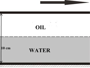
International Conference on Computation in Science and Engineering IOP Publishing
IOP Conf. Series: Journal of Physics: Conf. Series 1090 (2018)
 1234567890 ‘’“” 012050 doi:10.1088/1742-6596/1090/1/012050

Numerical solutions to a parabolic model of two-layer fluids

 Sudi Mungkasi and Friska Dwi Mesra Mangadil
 Department of Mathematics, Faculty of Science and Technology,
 Sanata Dharma University, Yogyakarta, Indonesia

 E-mail: sudi@usd.ac.id

 Abstract. In this paper, we consider the motion of two layers of fluids having different
 viscosity values. The motion is driven by a moving surface, but the bottom is fixed. An exact
 analytical solution for unsteady state cases is not available. Therefore, a numerical method
 should be used for the solution to unsteady state cases of the problem. In this work, we propose
 a finite volume numerical method to find the numerical velocity of the problem. We use the
 Lax-Friedrichs formulation for the flux calculation. Our numerical results show that fluids
 move following the motion of the surface. In addition, the fluid at the top layer moves faster
 than the bottom layer fluid. These behaviour is correct with respect to the physical problem
 under consideration.

1. Introduction
Numerical simulation has been widely used by mathematical modellers to investigate physical
phenomena. The phenomena is first modelled into a system of equations. The system is then solved
numerically, as the exact analytical solution is generally difficult to find.
 This paper considers the problem of two layers of fluids moving in one direction. We assume that
oil layer is on the top of water layer. The two layers are in between a moving surface and a fixed
bottom. The moving surface has a constant velocity. This problem was introduced by Caldwell and
Ng [1], who used a finite difference method to obtain its numerical solution.
 In this work, we provide an alternative numerical solver by proposing a finite volume method to
find the numerical solution to the problem. The finite volume method works well as long as the
mathematical model can be written in a conservative form. We implement the Lax-Friedrichs
formulation [2-3] to compute numerical fluxes of the conservative form of the model. Our numerical
scheme is explicit. As time tends to infinity, the motion of fluids is steady. This is confirmed by the
exact as well as the numerical solution. The numerical solution agrees quite well with the exact steady
state solution.
 The rest of this paper is organised as follows. We present the problem formulation in Section 2.
Numerical method is proposed in Section 3. We provide numerical results in Section 4. The paper is
concluded in Section 5.

2. Problem formulation
This section introduces the equations for the motion of the two-layer fluids.
 Consider two horizontal plates with a distance of 10 cm and between those two plates there are oil
and water layers, as shown in Figure 1. The top plate moves to the right with a constant velocity. The
bottom plate is fixed. We assume that starting at time = 0, the top plate moves with constant
velocity 7 cm/s.

 Content from this work may be used under the terms of the Creative Commons Attribution 3.0 licence. Any further distribution
 of this work must maintain attribution to the author(s) and the title of the work, journal citation and DOI.
Published under licence by IOP Publishing Ltd 1

International Conference on Computation in Science and Engineering IOP Publishing
IOP Conf. Series: Journal of Physics: Conf. Series 1090 (2018)
 1234567890 ‘’“” 012050 doi:10.1088/1742-6596/1090/1/012050

 Figure 1. Two plates spaced 10 cm apart.

 This problem has been modelled mathematically by Caldwell and Ng [1] as:

 ∂ &'()* - &'()*
 = &'()* , (1)
 -
and
 123 - 123
 = 123 . (2)
 -

Here &'()* , is the velocity of water, 123 , is the velocity of oil, &'()* is the viscosity of
water, and 123 is the viscosity of oil. The free variables are time and space . The space is the fluid
height measured from the bottom. At the oil-water interface, we have the following relations:

 123 = &'()* , (3)
and
 123 &'()*
 123 = &'()* . (4)
 
 The simulation is conducted to determine the velocity of fluids at any time > 0, especially for a
large time , when the steady state is achieved.

3. Numerical method
In this section we present a complete mathematical model and the finite volume method that we
propose to solve the problem.
 The mathematical model is given in the following two sets of initial-boundary value problems:

 ∂ &'()* - &'()*
 = &'()* ,0 ≤ ≤ 6
 -

 &'()* , 0 = 0

 &'()* 0, = 0
 (5)
 &'()* 6, = 123 6, 

 123 &'()*
 123 = &'()*
 89: 89:

 2

International Conference on Computation in Science and Engineering IOP Publishing
IOP Conf. Series: Journal of Physics: Conf. Series 1090 (2018)
 1234567890 ‘’“” 012050 doi:10.1088/1742-6596/1090/1/012050

 123 - 123
 = 123 , 6 ≤ ≤ 10
 -

 123 , 0 = 0

 123 10, = 7 (6)

 123 6, = &'()* 6, 

 123 &'()*
 123 = &'()*
 89: 89:

The problem (5) and (6) can be solved separately, because there are some conditions that relate to each
other.
 In order to use the finite volume method, we rewrite equations (5) and (6) as:

 ∂ &'()* - &'()*
 − &'()* =0, (7)
 -

 ∂ 123 - 123
 − 123 =0. (8)
 -

Therefore, we have

 ∂ &'()* &'()*
 − &'()* =0, (9)
 
 ∂ 123 123
 − 123 =0. (10)
 
In compact forms, we write equations (9) and (10) as

 &'()*> + − &'()* &'()*@ =0, (11)
 8

 123> + − 123 123@ =0. (12)
 8

Equations (11) and (12) are in the form of conservation laws, that is, in their conservative forms:

 &'()*> + ( &'()* )8 = 0 , (13)

 123> + 123 8 =0. (14)

where &'()* = − &'()* &'()*@ and 123 = − 123 123@ respectively.

 Equation (13) is solved using the finite volume method with an explicit numerical scheme:

 ∆ F F
 &'()* FGH = &'()* FE − H − &'()* H . (15)
 E ∆ &'()* EG- EK
 -

 3

International Conference on Computation in Science and Engineering IOP Publishing
IOP Conf. Series: Journal of Physics: Conf. Series 1090 (2018)
 1234567890 ‘’“” 012050 doi:10.1088/1742-6596/1090/1/012050

Here,

 &'()* FE ≈ &'()* E , F and &'()* FEGH/- ≈ ( &'()* ( EGH/- , F ))

are the conserved quantity and the flux function, respectively. Here ∆ is time step and ∆ is space
step, is notation for the space index and is notation for the time index. To compute fluxes in
equation (15), we use the Lax-Friedrichs formulation:

 &'()* FE − &'()* FEKH ∆ 
 &'()* F H = − F
 − &'()* FEKH , (16)
 HK
 - 2 2∆ &'()* E

and

 &'()* FEGH − &'()* FE ∆ 
 &'()* F H = − F
 − &'()* FE . (17)
 HG
 - 2 2∆ &'()* EGH

 Analogously, equation (14) is solved using the finite volume method with an explicit scheme:

 ∆ 
 123 FGH
 E
 = 123 FE − 123 F H − 123 F H . (18)
 ∆ EG
 -
 EK
 -

To compute fluxes in equation (18), we use the Lax-Friedrichs formulation:

 123 FE − 123 FEKH ∆ 
 123 F H = − F − 123 FEKH , (19)
 HK
 - 2 2∆ 123 E

and

 123 FEGH − 123 FE ∆ 
 123 F H = − F − 123 FE . (20)
 HG
 - 2 2∆ 123 EGH

The finite volume schemes (15)-(17) and (18)-(20) are iterated with consideration of the initial and
boundary conditions given in equations (5)-(6). The iterations result in numerical solutions for the
fluid velocities. Note that another approach of finite volume method is available, for example, the
relaxation system [4-6], but it doubles the number of equations to be solved. Our finite volume method
in this paper is simpler than those relaxation approach.

4. Numerical results
In this section we present some representatives of our numerical results. The numerical results are
compared with a known analytical exact solution.
 As the benchmark, we recall the analytical exact solution obtained by Caldwell and Ng [1] as
follows. First considering
 Q R STUVWX
 =0, 0≤ ≤6, (21)
 Q8 R

with

 &'()* 0 = 0 , (22)

we get

 4

International Conference on Computation in Science and Engineering IOP Publishing
IOP Conf. Series: Journal of Physics: Conf. Series 1090 (2018)
 1234567890 ‘’“” 012050 doi:10.1088/1742-6596/1090/1/012050

 &'()* = + . (23)

Because &'()* 0 = 0 , then = 0. Equation (23) becomes:

 &'()* = , 0 ≤ ≤ 6 . (24)

The steady state case for oil requires

 Q R S[\]
 = 0 , 6≤ ≤ 10 , (25)
 Q8 R
with
 123 10 = 7 , (26)

 123 6 = &'()* 6 , (27)

 123 &'()*
 123 = &'()* . (28)
 89: 89:

Then we get:

 123 = + , 6≤ ≤ 10 . (29)

The conditions (26) and (27) lead to

 10 + = 7 , (30)

 6 + = 6 . (31)

 `S[\] `STUVWX
Because = and = , we write
 `8 `8

 123 ( ) = &'()* ( ). (32)

Equation (30)-(32) can be solved to obtain:

 7 123
 = (33)
 6 123 + 4 &'()*

 7 &'()* (34)
 =
 6 123 + 4 &'()*

 21 ( 123 − &'()* )
 = (35)
 3 123 + 2 &'()*

Finally, the exact steady state solutions are:

 cd[\]
 &'()* = , 0≤ ≤6, (36)
 :d[\] GedTUVWX

 cdTUVWX -H (d[\] KdTUVWX )
 123 = + , 6≤ ≤ 10 . (37)
 :d[\] GedTUVWX fd[\] G-dTUVWX

 5

International Conference on Computation in Science and Engineering IOP Publishing
IOP Conf. Series: Journal of Physics: Conf. Series 1090 (2018)
 1234567890 ‘’“” 012050 doi:10.1088/1742-6596/1090/1/012050

 Figure 2. Large time behaviour of velocity of two fluid layers, at time = 100 s.

 Numerical setting in this simulation is as follows. We assume that &'()* = 1 cp and 123 = 3 cp.
The cell width or also known as the space step is ∆ = 0.1. The time step is ∆ = 0.001 ∙ ∆ . The
simulation is stop at the final time = 100 s. Here we want to see that change of velocity of two-fluid
layers from = 0 to = 10 when the steady state is achieved. Note that the -axis is vertical, instead
of horizontal.
 Our numerical results show that the numerical method solves the problem successfully. The main
source of numerical error is at the non-smooth trasition between the oil and water layers, that is, the
oil-water interface. At this interface, the fluid viscosity is discontinuous. However, we can have
smaller error if we take smaller cell width and smaller time step. A representative of our numerical
results is shown in Figure 2. The numerical results is correct physically. The velocity values get larger
from the bottom to the top surface. This phenomena is identified in both the analytical and numerical
solutions.

5. Conclusion
We have proposed a finite volume numerical method to solve the problem of two layers of fluids
driven by a horizontally moving surface with fixed bottom. The numerical method can be used to
solve both steady and unsteady state problems. Accurate solution can be obtained using a fine
numerical mesh, that is, fine cell width and fine time step. Our research results are limited to one-
dimensional problems. Future research direction could be an extension to higher dimensional
problems.

 6

International Conference on Computation in Science and Engineering IOP Publishing
IOP Conf. Series: Journal of Physics: Conf. Series 1090 (2018)
 1234567890 ‘’“” 012050 doi:10.1088/1742-6596/1090/1/012050

Acknowledgements
The work of Sudi Mungkasi was financially supported by DRPM of Ditjen Penguatan Riset dan
Pengembangan of Kementerian Riset, Teknologi, dan Pendidikan Tinggi of The Republik of Indonesia
in year 2017 with Research Contract Number 051/HB-LIT/IV/2017 dated on 14 April 2017 (under
DIPA-042.06-0.1.401516/2017 funds).

References
 [1] Caldwell J and Ng D K S 2004 Mathematical Modelling: Case Studies and Projects (New
 York: Kluwer Academic Publishers)
 [2] LeVeque R J 1992 Numerical Methods for Conservation Laws (Basel: Springer)
 [3] LeVeque R J 2002 Finite Volume Methods for Hyperbolic Problems (Cambridge: Cambridge
 University Press)
 [4] Banda M K and Herty M 2012 Adjoint IMEX-based schemes for control problems governed by
 hyperbolic conservation laws Computational Optimization and Applications 51 909
 [5] Jin S and Xin Z 1995 The relaxation schemes for systems of conservation laws in arbitrary
 space dimensions Communications on Pure and Applied Mathematics 48 235
 [6] Yohana E M and Banda M K 2016 High-order relaxation approaches for adjoint-based optimal
 control problems governed by nonlinear hyperbolic systems of conservation laws Journal of
 Numerical Mathematics 24 45

 7