Occipital condyle width (OCW) is a highly accurate predictor of body mass in therian mammals
←
→
Page content transcription
If your browser does not render page correctly, please read the page content below
Engelman BMC Biology        (2022) 20:37
https://doi.org/10.1186/s12915-021-01224-9

 RESEARCH ARTICLE                                                                                                                                  Open Access

Occipital condyle width (OCW) is a highly
accurate predictor of body mass in therian
mammals
Russell K. Engelman

  Abstract
  Background: Body mass estimation is of paramount importance for paleobiological studies, as body size influences
  numerous other biological parameters. In mammals, body mass has been traditionally estimated using regression
  equations based on measurements of the dentition or limb bones, but for many species teeth are unreliable
  estimators of body mass and postcranial elements are unknown. This issue is exemplified in several groups of
  extinct mammals that have disproportionately large heads relative to their body size and for which postcranial
  remains are rare. In these taxa, previous authors have noted that the occiput is unusually small relative to the skull,
  suggesting that occiput dimensions may be a more accurate predictor of body mass.
  Results: The relationship between occipital condyle width (OCW) and body mass was tested using a large dataset
  (2127 specimens and 404 species) of mammals with associated in vivo body mass. OCW was found to be a strong
  predictor of body mass across therian mammals, with regression models of Mammalia as a whole producing error
  values (~ 31.1% error) comparable to within-order regression equations of other skeletal variables in previous
  studies. Some clades (e.g., monotremes, lagomorphs) exhibited specialized occiput morphology but followed the
  same allometric relationship as the majority of mammals. Compared to two traditional metrics of body mass
  estimation, skull length, and head-body length, OCW outperformed both in terms of model accuracy.
  Conclusions: OCW-based regression models provide an alternative method of estimating body mass to traditional
  craniodental and postcranial metrics and are highly accurate despite the broad taxonomic scope of the dataset.
  Because OCW accurately predicts body mass in most therian mammals, it can be used to estimate body mass in
  taxa with no close living analogues without concerns of insufficient phylogenetic bracketing or extrapolating
  beyond the bounds of the data. This, in turn, provides a robust method for estimating body mass in groups for
  which body mass estimation has previously been problematic (e.g., “creodonts” and other extinct Paleogene
  mammals).
  Keywords: Body size, Mass estimation, Allometry, Non-linear regression, Non-linear allometry

Background                                                                            [6], longevity [7], reproductive rate [8], home range size
Body size (body mass) is a particularly important feature                             [9], degree of sexual size dimorphism [10], relative brain
of an organism’s biology, as it is correlated with dietary                            size [11, 12], morphology and degree of morphological
habits [1–4], basal metabolic rate [5], population density                            specialization [13], defensive behavior [14], guild struc-
                                                                                      ture [15, 16], isotope enrichment ratios [17], and extinc-
                                                                                      tion risk [18], among various other factors (see [19–21]
Correspondence: neovenatoridae@gmail.com
Department of Biology, Case Western Reserve University, 10900 Euclid
                                                                                      and references therein). Indeed, many authors have gone
Avenue, Cleveland, OH 44106, USA                                                      so far as to say that body mass is the single most
                                       © The Author(s). 2022 Open Access This article is licensed under a Creative Commons Attribution 4.0 International License,
                                       which permits use, sharing, adaptation, distribution and reproduction in any medium or format, as long as you give
                                       appropriate credit to the original author(s) and the source, provide a link to the Creative Commons licence, and indicate if
                                       changes were made. The images or other third party material in this article are included in the article's Creative Commons
                                       licence, unless indicated otherwise in a credit line to the material. If material is not included in the article's Creative Commons
                                       licence and your intended use is not permitted by statutory regulation or exceeds the permitted use, you will need to obtain
                                       permission directly from the copyright holder. To view a copy of this licence, visit http://creativecommons.org/licenses/by/4.0/.
                                       The Creative Commons Public Domain Dedication waiver (http://creativecommons.org/publicdomain/zero/1.0/) applies to the
                                       data made available in this article, unless otherwise stated in a credit line to the data.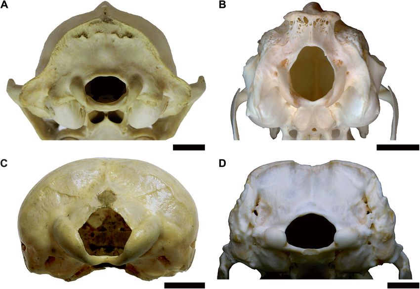
Engelman BMC Biology   (2022) 20:37                                                                         Page 2 of 44

important aspect of the biology of any organism [22–         associated with craniodental material [62–65; E. Davis,
29]. As a result, estimations of body mass are of extreme    pers. comm., 2018]. Even if postcranial remains are bet-
importance when studying the paleobiology and                ter predictors of body mass in mammals, it is a moot
paleoecology of a given species, both in terms of how it     point in terms of estimating body mass if no postcrania
affects the taxon’s biology and how the taxon interacts      are known for the taxon.
with other species in its community.                           This scarcity of postcranial remains particularly hin-
   The most common method of estimating body mass            ders attempts to use HBL to estimate body mass, a
in extinct animals is to use a regression equation based     measurement which has otherwise been suggested to be
on skeletal measurements and body mass from a com-           one of the best estimators of body mass in fossil mam-
parative sample of closely related extant species (which     mals [52, 66]. HBL can only be accurately measured on
are often assumed to have geometric similarity). For fos-    a nearly complete, undistorted skeleton with a complete
sil mammals, these estimates are often based on teeth,       spinal column and as a result can only be applied to ex-
which are commonly preserved [30] and are often the          tremely well-known taxa [67, 68] (see also Sarko et al.
only fossil remains known for many species. However,         [69] for discussion of a comparable issue in sirenians).
regression equations based on teeth can be problematic       Even well-preserved taxa are often missing one or more
when trying to apply them to mammals that have no            vertebrae and must be reconstructed by filling in missing
close living relatives [31, 32]. Furthermore, many of        parts with ones based on those of close relatives, which
these extinct animals may exhibit dental morphologies,       can affect body mass estimates. For example, Sinclair
body proportions, and patterns of allometric scaling un-     [33] originally restored the sparassodont Borhyaena
like any living species. For example, many groups of ex-     tuberata with parts of Prothylacynus patagonicus and
tinct mammals have disproportionately large heads            Thylacinus cynocephalus, whereas Argot [70] restored B.
relative to extant species (Fig. 1). This phenomenon has     tuberata with a much shorter torso and longer limbs
been most extensively discussed in extinct carnivorous       based on extrapolation from the known limb and verte-
mammals, such as sparassodonts [35, 36], mesonychians        bral dimensions of this taxon. Using the all-taxon HBL
[37], and oxyaenid [38] and hyaenodont [32, 39] “creo-       regression equation for carnivorous mammals in Van
donts,” as well as some extinct carnivorans such as          Valkenburgh [39], the reconstruction of B. tuberata in
amphicyonids [40, 41] and nimravids [39]. However, this      Sinclair [33] produces a body mass estimate of 22.88 kg
condition also occurs in pantodonts [42, 43], “condy-        whereas that in Argot [70] using the same equation pro-
larths” [44], taeniodonts [45], entelodonts [46], diproto-   duces a body mass estimate of 18.36 kg, nearly 5 kg (or
dontoid marsupials [47], South American endemic              20%) lighter. Another issue is that HBL includes the
ungulates [48–52], large-bodied rodents [53, 54], and        length of the cranium as well as the body as a part of
Malagasy subfossil lemurs [55], among others. Given the      formulating this measurement. Thus, HBL is influenced
disproportionately large heads of these taxa, body mass      by skull size in the same manner as craniodental mea-
estimates based on craniodental regression equations de-     surements and can produce unreliable body mass esti-
rived from modern taxa are thought to overestimate           mates in large-headed mammals [32, 56].
body mass (see [32, 39, 56]).                                  Furthermore, although postcranial body mass esti-
   Because of these difficulties with craniodental mea-      mates are often regarded as being more independent of
surements many authors have considered head-body             phylogeny or biology than craniodental measurements,
length (HBL) or postcranial measurements such as the         limb bone dimensions are still influenced by these fac-
length, diameter, or cross-sectional area of long bone di-   tors. Good example of this are xenarthrans and cavio-
aphysis or articular surfaces of limb bones to be better     morph rodents, which have disproportionately robust
estimators of body mass [32, 55, 57–59]. However, body       hindlimbs relative to their body size [31, 71], likely be-
mass estimates based on postcranial measurements             cause these animals often feed or mate in a bipedal
present their own difficulties, which have often been        stance and therefore must occasionally support all of
under-appreciated and rarely discussed in the literature.    their weight on their hindlimbs [71–73], which violates
Perhaps most importantly, the postcranium in most spe-       the assumption that weight is being distributed in a
cies of fossil mammals is either poorly known or repre-      comparable manner across the fore- and hindlimbs in
sented by very fragmentary material, and the postcranial     Mammalia. In particular, Millien and Bovy [31] found
anatomy of even some higher-level clades remains more        that extinct giant caviomorphs like Phoberomys patter-
or less unknown (e.g., the notoungulate family Archaeo-      soni have hindlimb bones that are disproportionately ro-
hyracidae [60, 61]). This is because taxonomic diagnoses     bust to their body size even relative to extant
of most extinct mammal are almost exclusively based on       caviomorphs, which according to these authors may
craniodental features, with postcranial remains usually      have produced inaccurate body mass estimates for this
only identified to genus or species if they directly         taxon. This is demonstrated in the fact that, due to their
Engelman BMC Biology        (2022) 20:37                                                                                                Page 3 of 44

 Fig. 1 Skeletal reconstructions of a borhyaenid sparassodont (A, Borhyaena tuberata; modified from Sinclair [33]), hyaenodont “creodont” (B,
 Hyaenodon horridus; modified from Scott and Jepsen [34]), and canid carnivoran (C, Canis lupus, public domain from Wikimedia Commons),
 scaled to the same thorax length (not head-body length, due to differences in relative neck length in the three taxa), illustrating the
 proportionally larger heads of Borhyaena and Hyaenodon
Engelman BMC Biology    (2022) 20:37                                                                           Page 4 of 44

unusually robust hindlimbs, body mass estimates for           the fact that the equations used to calculate these esti-
glyptodonts and extinct giant caviomorphs like Phober-        mates were based on perissodactyls and artiodactyls,
omys based on the femur range from 70 to 380% higher          which phylogenetically bracket litopterns and notoungu-
than estimates based on the humerus [74, 75]. Com-            lates [89, 90]. As a result, when estimating the body
pounding problems with the influence of ecology or            mass of species belonging to wholly extinct groups, it is
phylogenetic signal is the fact that most extant large        critical to use variables that can be confidently applied
mammals, such as artiodactyls, equids, many carnivor-         across Mammalia more generally and are not specific to
ans, and even rhinocerotids to some degree [76, 77], are      a particular group.
cursorial and have relatively gracile limbs. By contrast,        Because of these issues, interest in potential alternative
most of the extinct mammal groups that researchers are        methods of estimating body mass in mammals has been
frequently interested in estimating body mass for, such       steadily increasing. Recent studies have suggested that
as “creodonts” [78, 79], sparassodonts, mesonychians          dimensions of the scapula [91], astragalus [58, 92], and
[37], pantodonts [80], extinct Paleogene or South Ameri-      calcaneus [93] may all be strong predictors of body
can ungulates [50, 52, 81], caviomorph rodents [31],          mass. Another potential alternative to traditional cranio-
xenarthrans [74, 82], tend to be more ambulatory and          dental and postcranial-based methods of estimating body
have more robust limbs than extant large mammals. As          mass, especially for the aforementioned extinct “large-
a result, the limb dimensions of large extant mammals         headed” taxa, are dimensions of the occiput. Argot and
may not reflect the proportions of extinct taxa, and this     Babot [94] noted that although the heads of the hyaeno-
is likely to cause errors in body mass estimation if the      dont “creodont” Hyaenodon and the sparassodont Calli-
two are assumed to be directly comparable [31, 32, 37,        stoe are relatively large for their body size, the occiput
74, 82].                                                      appeared unusually small, resembling the overall dispar-
  A related issue is one of phylogenetic bracketing.          ity in size between the cranium and postcranium in
Phylogenetic bracketing is a key concept in modern            these taxa. This suggests that dimensions of the occiput
paleontology, for if a biological inference can be applied    may scale with the size of the postcranium, rather than
to two distinct branches of a phylogeny, it also likely ap-   the cranium, and therefore may be a more accurate
plies to the extinct taxa between them as well [83]. How-     proxy of body size than other craniodental measure-
ever, many prior studies estimating body mass in wholly       ments, particularly in these large-headed extinct
extinct groups of mammals often estimate mass based           mammals.
on regression equations derived (often by necessity)             There are several reasons to believe that occiput di-
from unrelated species that do not bracket the taxon of       mensions may be good estimators of body size. Because
study. For example, body masses in “creodonts” and            the atlanto-occipital joint is the link between the post-
sparassodonts have often been estimated based on re-          cranium and cranium, dimensions of the occiput might
gression equations derived from distantly related carni-      be expected to more closely correlate with postcranial
vorans, didelphimorphians, and dasyuromorphians (e.g.,        proportions than other craniodental measurements, as
[32, 39, 84]), and body masses in extinct hyracoids and       the occiput is constrained by the size of the spinal col-
South American ungulates have typically been estimated        umn. The occiput also shares a common developmental
based on regression equations derived from perissodac-        origin with the vertebral column separate from the rest
tyls and artiodactyls (e.g., [81, 85, 86]). Very rarely do    of the skull, as the post-otic region of the skull (includ-
studies examine if the relationships in their regression      ing the occiput) is formed by the incorporation of the
equations can be more broadly applied across Mammalia         anteriormost trunk somites into the cranium [95, 96].
or are only applicable within their respective clade (with    Hence, the dimensions of the occiput can be thought of
some exceptions including [58, 87, 88]).                      as postcranial landmarks measurable on the cranium. All
  Even when phylogenetic bracketing is present it may         of the nerves that innervate the postcranium (with the
not be sufficient if the variables are not broadly applic-    exception of the vagus nerve) pass through the foramen
able. For example, McGrath et al. [81] noted that both        magnum, in addition to the vertebral arteries, anterior
postcranial and craniodental variables failed to produce      and posterior spinal arteries, tectorial membranes, and
reliable body mass estimates in macraucheniid litop-          alar ligaments, among other structures. Given that the
terns, due to unique features of macraucheniids (robust       number of neurons per unit mass of postcranial body
limbs and complete, closed dentitions) that are not           tissue is relatively consistent within mammals [97], this
present in most extant ungulates. Similarly, Croft et al.     means that the size of the foramen magnum and its sur-
[52] found that craniodental equations likely overesti-       rounding structures (i.e., the occiput) would be expected
mated body mass in notoungulates due to characteristics       to closely correlate with body size (but see [98]).
of notoungulates not present in modern ungulates                 More broadly, the postcranium of most terrestrial
(namely large heads relative to body size). This is despite   mammals is also relatively conservative, with most
Engelman BMC Biology     (2022) 20:37                                                                             Page 5 of 44

species exhibiting a relatively short neck with seven cer-       during prey capture, inter/intraspecific combat, or other-
vical vertebrae, 19–20 thoracolumbar vertebrae [99], a           wise interacting with a resistant object) due to the nar-
reduced or absent tail that contributes little to body           rower distance between the condyles relative to the
mass compared to other chordates, and four limbs of              anteroposterior length of the skull resulting in a less
roughly comparable size. Specifically, with regard to the        stable joint. This would be even more pronounced in
tail, mammals exhibit a reduction in overall tail robust-        large-headed species because the moment arm (the an-
ness compared to other tetrapods [100], driven by fac-           teroposterior length of the skull) is inherently longer.
tors such as a more gracile caudal skeleton, a reduction         Therefore, if an animal has an occiput that is small rela-
of caudal musculature such as the reptilian caudofemor-          tive to skull size, it is more likely that the animal merely
alis, and the fact that, unlike limbed squamates and             has a disproportionately large head, with the occiput di-
crocodilians, most mammals do not use the tail as a              mensions being constrained by the size of the spinal col-
major fat-storing organ (with some exceptions, see               umn, rather than the animal having a disproportionately
[101]). The reptilian caudofemoralis alone (which is not         small occiput relative to its body. This agrees with what
homologous to the caudofemoralis muscle in mammals               is observed in taxa like Callistoe and Hyaenodon.
and is actually absent in the latter) comprises about 1/3           One measurement of the occiput that may prove par-
of total caudal muscle mass in most non-avian saurop-            ticularly useful for estimating body mass in fossil mam-
sids and in Iguana iguana represents ~ 3.6% of total             mals is occipital condylar width (hereafter abbreviated as
body weight ([100, 102]). In non-avian sauropsids, the           OCW). Martin [116] used OCW to estimate body mass
tail is typically 20% or more of total body mass (Table          in extinct mammals; however, these regressions were
1), whereas even in mammals with relatively long, mus-           based on a relatively small (N = 26), taxonomically re-
cular tails like Ateles the tail is no more than 8% of the       stricted sample. After Martin [116], only a few studies
total body mass (and it is typically less than 5% in mam-        have used dimensions of the occipital condyles to esti-
mals without prehensile tails). As a result, the body pro-       mate body mass in extinct terrestrial mammals [65,
portions of mammals are less variable than those of              117–121]. OCW has been used more frequently to pre-
most other tetrapods and thus there are fewer poten-             dict body mass in marine mammals (cetaceans, [122–
tially confounding variables when estimating body size           124]; sirenians, [69, 125]; pinnipeds, [126, 127]). This is
based on axial dimensions (e.g., variation in tail size, pre-    in stark contrast to the large number of studies that have
sacral vertebral counts, or bipedalism versus quadru-            estimated body mass of terrestrial mammals via dimen-
pedalism in reptiles [22, 112, 113];).                           sions of postcrania, teeth, and measurements such as
   Additionally, there is likely to be very strong stabilizing   HBL or skull length. Many multivariate studies of body
selection on the occiput. Maintaining function of the            mass based on craniodental or whole-body metrics do
atlanto-occipital joint is critical for an individual’s fit-     not even consider dimensions of the occiput outside of
ness, as luxation of this joint is almost invariably fatal       occiput height [86, 128]. The applicability of OCW
[114]. Any mutation that compromised occiput function            across mammals more generally has never been tested,
would be rapidly removed from the gene pool and as a             though it has been suggested [129]. In this study, I
result morphological change in this structure due to             examine the allometric relationship between OCW and
genetic drift would be low. This suggests that occiput           body mass in a wide range of extant mammals, calculate
evolution would be highly conservative and thus the oc-          regression equations based on these data, and compare
ciput may be a good proxy for estimating body mass               the accuracy of these regression equations with previous
across a broad range of mammals. While it would be               studies.
theoretically possible for selection to favor an occiput
that is disproportionately large relative to body size (as       Results
might be expected if there were very strong stresses at          Data distribution and model fitting
the atlanto-occipital joint, such as perhaps in some             A strong correlation exists between OCW and body
horned artiodactyls; [115]), it is unlikely that many ani-       mass (Fig. 2). However, the relationship between the two
mals would have occiputs that are disproportionately             variables is not log-linear. Instead, plotting ln OCW
small relative to body size. This is because if an animal        against ln body mass shows the points form a curvilinear
had a disproportionately small occiput relative to its           distribution that is slightly concave down, with larger
head and body it would result in a greater amount of             mammals having proportionally larger OCW relative to
force being applied to a smaller joint surface and thus          body size (Fig. 2). This is supported by a general obser-
increase the risk of atlanto-occipital luxation. Addition-       vation made during data collection that larger taxa had
ally, a smaller occiput would result in greater transverse       proportionally larger occipital condyles. For example, in
torque at the atlanto-occipital joint when mediolateral          the present study, the occipital condyles represent a pro-
forces are applied at the anterior end of the skull (as in       portionally smaller part of OCW in smaller mammals
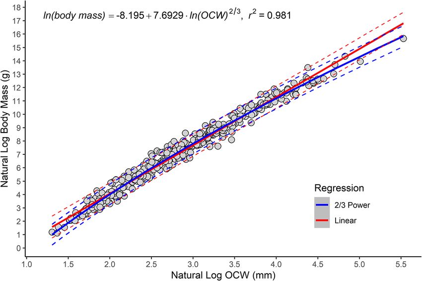
Engelman BMC Biology         (2022) 20:37                                                                                Page 6 of 44

Table 1 Comparison of tail masses as a percent of total body mass in mammals and non-mammalian tetrapods. Note that the
available data for mammals is disproportionately focused on taxa with large tails (Macropodiformes and prehensile-tailed taxa), the
average mammal (e.g., Canis, Felis, Peromyscus) typically has a much smaller tail
Taxon                                       Group               Family                         % Tail mass                 Reference
Alligator mississippiensis                  Sauropsida          Alligatoridae                  24.5%                       [103]
Alligator mississippiensis                  Sauropsida          Alligatoridae                  27.8%                       [104]
Iguana iguana                               Sauropsida          Iguanidae                      18.8%                       [102]
Christinus marmoratus                       Sauropsida          Gekkonidae                     20–24%                      [105]
Eublepharis macularius                      Sauropsida          Gekkonidae                     22%                         [106]
Plethodon cinereus                          Caudata             Plethodontidae                 15–20%                      [107]
Macaca fascicularis                         Mammalia            Cercopithecidae                4%                          [108]
Macaca fuscata                              Mammalia            Cercopithecidae                0.1%                        [108]
Macaca nemestrina                           Mammalia            Cercopithecidae                0.2%                        [108]
Ateles sp.                                  Mammalia            Atelidae                       7.8%                        [108]
Alouatta caraya                             Mammalia            Atelidae                       5.5%                        [108]
Cebus sp.                                   Mammalia            Cebidae                        5.4%                        [108]
Saguinus Oedipus                            Mammalia            Callitrichidae                 3.0%                        [108]
Aotus trivirgatus                           Mammalia            Aotidae                        4.2%                        [108]
Perodicticus potto                          Mammalia            Lorisidae                      0.4%                        [108]
Otolemur crassicaudatus                     Mammalia            Galagidae                      4.3%                        [108]
Galago senegalensis                         Mammalia            Galagidae                      2.5%                        [108]
Tupaia glis                                 Mammalia            Tupaiidae                      2.6%                        [108]
Dasyprocta aguti                            Mammalia            Caviidae                       < 0.1%                      [102]
Dolichotis salinicola                       Mammalia            Caviidae                       0.0%                        [102]
Dinomys branickii                           Mammalia            Dinomyidae                     1.1%                        [109]
Erethizon dorsatum                          Mammalia            Erethizontidae                 3.3%                        [109]
Coendou prehensilis                         Mammalia            Erethizontidae                 8.7%                        [109]
Peromyscus maniculatus                      Mammalia            Cricetidae                     1.0–4.0%                    [110]
Canis familiaris                            Mammalia            Canidae                        0.4%                        [108]
Felis catus                                 Mammalia            Felidae                        1.3%                        [108]
Bradypus variegatus                         Mammalia            Bradypodidae                   < 0.1%                      [102]
Choloepus hoffmanni                         Mammalia            Choloepodidae                  < 0.1%                      [102]
Didelphis marsupialis                       Mammalia            Didelphidae                    3.0%                        [108]
Macropus rufus                              Mammalia            Macropodidae                   7.0%                        [111]
Dendrolagus matschiei                       Mammalia            Macropodidae                   5.0%                        [111]
Potorous apicalus                           Mammalia            Potoroidae                     3.0%                        [111]
Pseudocheirus peregrinus                    Mammalia            Pseudocheiridae                7.0%                        [111]

like Reithrodontomys megalotis (27.9%) and Tarsipes ros-             the largest taxon in the dataset, Loxodonta africana,
tratus (35.4%), whereas in larger mammals like Cervus                which also exhibits one of the largest absolute residuals
canadensis (55.6%), Ursus americanus (48.4%), and                    under a log-linear regression model. The OCW of L. af-
Diceros bicornis (55.1%) the occipital condyles comprise             ricana is nearly 75 mm wider than would be predicted
a greater proportion of OCW.                                         based on a log-linear model (250 mm versus 175 mm),
   Assuming a log-linear model, the best-fit line system-            and body mass under a log-linear model is overesti-
atically overestimates body mass at the extremes of the              mated by 64% (Additional file 2). For Ursus maritimus,
dataset and underestimates values for taxa closer to the             the largest taxon in this dataset for which N > 2, the dif-
midpoint (Additional file 1). The effects of non-linearity           ference in predicted versus actual OCW is less extreme
in the data after log-transformation can be best seen in             (6 mm, or 7% of actual OCW), but still produces an
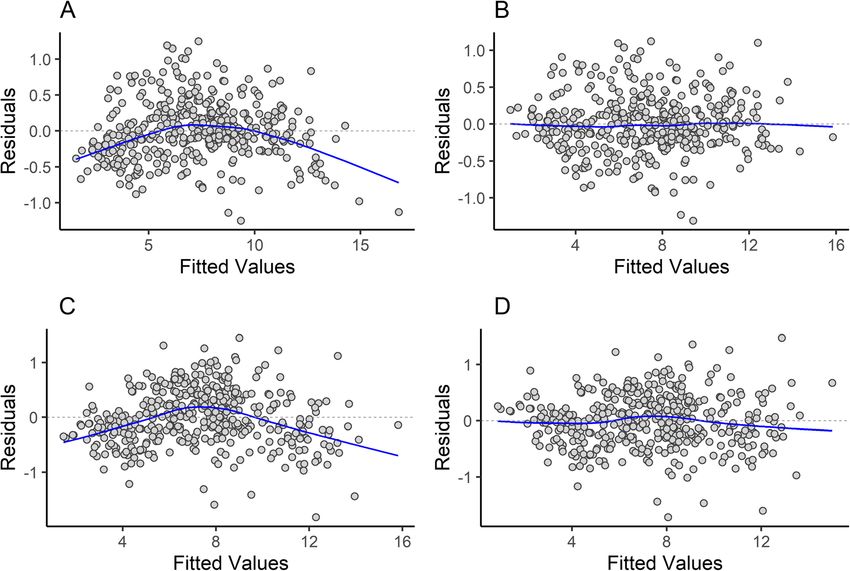
Engelman BMC Biology            (2022) 20:37                                                                                                          Page 7 of 44

  Fig. 2 Scatterplot of natural log of OCW versus natural log of body mass, showing the best fit (natural log OCW raised to the 2/3 power) regression
  line for all species and the non-linear distribution of the data. Linear regression is in red and 2/3 power regression is in blue. Dashed lines represent
  95% prediction intervals. Most of the species located above the upper bounds of the prediction interval are lagomorphs (see Fig. 7)

underestimate of body mass (especially compared to the                               to the 2/3 power significantly outperformed a log-linear
final non-linear model used here). The same issue is                                 one in terms of %PE, %SEE, log likelihood, AIC, and BIC
present for the smallest mammals in this study, though                               (Table 2). The next best-fitting model was a log-
is less obvious in magnitude due to the differences in                               quadratic model (Additional file 3), which had compar-
scales involved. Overall, however, the data seems to                                 able %PE and %SEE but higher log likelihood, AIC, and
curve significantly more at its upper extreme than its                               BIC. The residuals versus fits plot for a log-linear model
lower one.                                                                           between OCW and body mass shows a distinctly non-
  When comparing several different regression models,                                linear, heteroskedastic relationship (Fig. 3a), whereas
a log-power model in which natural log OCW was raised                                under a 2/3 power model (see Fig. 3b) or a log-quadratic

Table 2 Accuracy statistics for the regression model between natural log OCW and natural log body mass using the all taxon,
species average dataset under several different ordinary least squares (OLS) and phylogenetic least squares (PGLS) regression models
Method              Regression            AIC          BIC          logLik          df           r2adj           %PE           CF             %PEcf           %SEE
OLS                 Linear                441          453          − 217           402          0.9784          34.88         0.905          38.99           51.50
OLS                 1/2 power             409          421          − 201           402          0.9810          32.70         1.145          31.28           49.09
OLS                 1/3 power             455          467          − 224           402          0.9777          35.22         1.260          33.80           52.63
OLS                 2/3 power             389          401          − 192           402          0.9811          32.03         1.047          31.09           47.69
OLS                 3/4 power             391          403          − 193           402          0.9809          32.21         1.004          32.10           47.82
OLS                 Quadratic             391          407          − 192           401          0.9810          32.05         1.068          30.98           47.73
OLS                 Cubic                 393          413          − 191           400          0.9809          32.04         1.055          31.05           47.79
PGLS                Linear                420          432          − 207           402          –               70.12         1.725          34.30           309.11
PGLS                1/3 power             367          379          − 180           402          –               75.61         1.953          32.95           276.45
PGLS                2/3 power             368          380          − 181           402          –               68.88         1.754          31.56           276.00
PGLS (OU)           2/3 power             394          406          − 194           402          –               32.00         1.046          31.08           47.45
Abbreviations: PGLS (OU), phylogenetic least squares under an Ornstein-Uhlenbeck model (rather than Brownian); AIC, Akaike Information Criterion; BIC, Bayesian
Information Criterion; logLik, log likelihood; df, degrees of freedom; r2adj, adjusted r2 value; %PE, percent prediction error; CF, averaged correction factor (see
“Methods”); %PEcf, percent prediction error after applying correction factor; %SEE, standard error of estimate
Engelman BMC Biology (2022) 20:37 Page 8 of 44
Fig. 3 Residuals versus fitted plot for the regression of OCW (A,B) or skull length (C,D) against body mass. A and C represent residuals versus
fitted graphs for regression lines where isometry is assumed, and B and D represent graphs with the natural log of the independent variable
raised to the 2/3 power (in B) or the 1/2 power (in D)
model this distribution is linearized. Empirical curve fit- confidence interval for the exponent (Table 3) rules out
ting of a power rule using the non-linear least squares a strictly linear regression line, though it cannot fully
(nls) function in R produced a model with an exponent rule out a 3/4 power scaling relationship. Comparing the
of 0.688 (Table 3), very close to the exponent expected if models under ANOVA found the log-quadratic and 2/3
the data scaled to the 2/3 power (0.667). The 95% power model to be non-significantly different (F =
Table 3 Results of non-linear curve fitting of OCW, CBL, and HBL. The first seven regression equations are regressing natural log
OCW, CBL, or HBL (x variables) against natural log body mass (y variable, in g). The last two equations are regressing natural log
OCW against natural log CBL and natural log HBL, respectively. All equations are written in the form ln(y) = a × ln(x)^b + c
a b C
Metric Value 95% CI Value 95% CI Value 95% CI
OCW 7.289 (5.780, 8.800) 0.688 (0.578, 0.771) − 7.724 (− 9.501, − 5.947)
OCW (therians only) 7.470 (5.958, 8.981) 0.679 (0.599,0.760) − 7.939 (− 9.709, − 6.168)
OCW (excluding taxa) 7.253 (5.931, 8.575) 0.694 (0.621, 0.767) − 7.767 (− 9.324, − 6.209)
OCW (all specimens treated independently) 6.852 (6.160, 7.544) 0.714 (0.671,0.757) − 7.235 (− 8.039, -6.431)
OCW (average of wild-caught specimens only) 7.694 (5.544, 9.843) 0.663 (0.551, 0.775) − 8.154 (− 10.619, − 5.690)
CBL 18.017 (8.059, 27.975) 0.435 (0.288, 0.581) − 26.885 (− 38.366, − 15.403)
HBL 3.747 (2.036, 5.457) 0.918 (0.759, 1.078) − 11.883 (− 15.170, − 8.596)
OCW versus CBL 1.001 (0.768, 1.234) 1.020 (0.907, 1.134) 1.446 (1.123, 1.770)
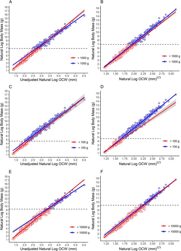
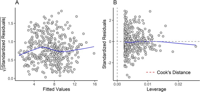
OCW versus HBL 2.631 (1.844, 3.418) 0.652 (0.536, 0.768) 0.713 (− 0.199, 1.626)Engelman BMC Biology (2022) 20:37 Page 9 of 44 0.3243, p = 0.5694), but the 2/3 power model is pre- data set (4430 g). Both slope (t = 3.083, p = 0.002) ferred here for reasons that will be detailed below. Un- and intercept (t = − 2.643, p = 0.008) significantly less otherwise mentioned, the results of this study refer differed between taxa above and below 100 g (Fig. to the model where log OCW is transformed by being 4d), but it is possible that this is due to the relatively raised to the 2/3 power before regression. smaller number of species less than 100 g in the The second-order term of the log-quadratic model present sample (N = 84, 20.8% of the total sample) significantly correlated with log body mass (t = − 7.384, and the relatively narrow size range spanned by these p < 0.001), whereas under a log-cubic model the quad- species compared to the other two size class analyses. ratic term remained significantly correlated (t = − 7.376, Even for taxa above 10 kg, which span a similar num- p < 0.001) but the cubic term did not (t = 0.424, p < ber of species (N = 96), the log range of body sizes 0.672). This suggests that the addition of a quadratic spanned by these taxa was much larger. term substantially improved model accuracy, but the addition of a cubic term is not statistically justifiable. Results of regression between OCW and body mass A major difference between the 2/3 power model and The regression equation between OCW and body mass the log-quadratic model is the distribution of leverage. has a percent prediction error (%PE) of 31.09 (Table 4). In the log-linear and 2/3 power model, leverage is rela- 41.6% of taxa have an estimated body mass within ± 20% tively evenly distributed across the data points, although of the actual value, whereas 81.4% of taxa have estimates data at the extreme ends of the x-axis have more lever- masses within ± 50% of the actual value. The median age (Additional file 2). By contrast, in the log-quadratic error (21.73%) is much lower than the mean error, sug- model, most of the points have almost no leverage, with gesting that error rates in the regression equation are only the points at the extreme ends of the axis influen- being inflated by outlier points with high error. This is cing the shape of the quadratic curve. It is this reason, supported by the distribution of the residuals (Fig. 5a). along with the fact that the shape of the log-quadratic Residuals of the regression equation are homoscedastic model is very sensitive to taxon inclusion and data dis- (Breusch-Pagal test for heteroscedasticity; BP = 0.13618; tribution (see below), that a simpler 2/3 power model is df = 1, p = 0.7121), as also indicated by the scale- preferred here. location plot (Fig. 6a), but have a slight positive skew When comparing log-linear regression lines for dif- primarily due to several taxa that exhibit occiput morph- ferent size classes (Fig. 4), the slope of the regression ology that deviates from the typical mammalian condi- line becomes noticeably shallower at larger body sizes, tion (Fig. 5a). Skewness (0.193) is relatively low (≤ |0.5|, indicating that log OCW increases at a greater rate [131]), indicating the distribution of the residuals are relative to body size at larger body sizes. These differ- roughly symmetrical. Excess kurtosis is 0.532, suggesting ences in slope are significant when the dataset is that the residuals are slightly leptokurtic (i.e., there are divided into all taxa greater than or less than 1 kg more observations closer to the mean than to the tails of (t = − 5.568, p < 0.001) and 10 kg (t = − 6.460, p < the distribution). 0.001), but not at 100 g (t = − 0.619, p = 0.5360). The residuals of the data are not normally distributed However, there is no obvious inflection point that according to a Shapiro-Wilk test (W = 0.98739, p = would suggest a threshold between different linear 0.0014). However, this is probably due to the sensitivity scaling models, as suggested by Economos [130], but of the Shapiro-Wilk test to departures from normality at rather a gradual change in slope. This, again, suggests large sample sizes, where even small departures from the relationship between the data is non-linear and normality will result in the sample failing the normality that a non-linear 2/3 power or log-quadratic model is test [132]. Visual inspection of a histogram of the resid- more appropriate than a log-linear one. uals shows the residuals follow a nearly normal distribu- Transforming log OCW by raising it to the 2/3 tion (Fig. 5a). Based on the large number of observations power resulted in this pattern of non-linear allometry (N = 404) and the central limit theorem (which states at being linearized. Under a 2/3 power model, when large sample sizes most bivariate independent distribu- comparing the regression lines formed by all taxa tions are close enough to normality for assumptions of above and below 1 kg finds both slope (t = 1.194, p = normality to hold), the distribution of the data is close 0.233) and intercept (t = − 0.270, p = 0.787) to be enough to normal to be used for regression [132]. The non-significantly affected by size class (Fig. 4b). The quantile-quantile plot of the residuals supports a normal same was true when comparing slope (t = − 1.081, p distribution of the residuals (Fig. 5b), though there is a = 0.281) and intercept (t = − 1.449. p = 0.148) for all slight deviation in the upper quantile due to a longer taxa above or below 10 kg (Fig. 4f). The thresholds negative tail. None of the species included in this dataset for these two bins were slightly lower or higher, re- exhibit a particularly high Cook’s distance in the resid- spectively, than the midpoint for body mass in the uals versus leverage plot, suggesting that none of the
Engelman BMC Biology         (2022) 20:37                                                                                                 Page 10 of 44

 Fig. 4 Comparison of scaling patterns for different size classes. A, C, E Log-linear scaling relationships; B, D, F Scaling relationships of the data
 where log OCW is transformed by raising it to the 2/3 power. A, B Scaling patterns for taxa above and below 1 kg. C, D Scaling patterns for taxa
 above and below 100 g. E, F Scaling patters for taxa above and below 10 kg

species (including those with specialized condyle morph-                      error as N increases (Additional file 4), though this effect
ology) significantly influence the regression model on                        is not strong. These results are likely a consequence of
their own (Fig. 6b).                                                          the way that sampling works. Drawing from smaller
  The absolute value of the residuals is significantly cor-                   sample sizes of species increases the influence of individ-
related with the sample size for each species (t = −                          ual variation on the mean value, but a single sampled in-
2.011, p = 0.045). However, the r2 value of this correl-                      dividual could by sheer random chance be close to the
ation is very low (0.010) and the slope is close to zero                      theoretical mean value for the species. By contrast, larger
(m = − 0.00633). Plotting the absolute value of the resid-                    sample sizes generally “average out” individual deviations
uals versus sample size does shows a general decrease in                      from the species average [133, 134]. Hence, there is not
Engelman BMC Biology          (2022) 20:37                                                                                                Page 11 of 44

Table 4 Results of the regressions of natural log OCW (in mm) against natural log body mass (in g)
Dataset                                 N        Equation                                               r2adj      %PE        CF        %PEcf    %SEE
All species                             404      ln(body mass) = 7.69289 × ln(OCW)   2/3
                                                                                           − 8.19502    0.9810     32.03      1.047     31.09    47.69
Therians only                           401      ln(body mass) = 7.70727 × ln(OCW)2/3 − 8.21527         0.9823     31.55      1.037     30.83    45.92
Excluding taxa                          374      ln(body mass) = 7.76568 × ln(OCW)   2/3
                                                                                           − 8.36414    0.9862     27.89      1.021     27.47    40.62
All species (N ≥ 6)                     170      ln(body mass) = 7.68862 × ln(OCW)2/3 − 8.18776         0.9785     29.77      1.065     28.69    43.99
All species (N ≥ 6), excluding taxa     160      ln(body mass) = 7.76999 × ln(OCW)   2/3
                                                                                           − 8.2391     0.9815     27.72      1.068     26.56    41.30
All species (N ≥ 10)                    75       ln(body mass) = 7.71479 × ln(OCW)2/3 − 8.19504         0.9901     22.57      1.041     22.53    32.76
All species (N ≥ 10), excluding taxa    73       ln(body mass) = 7.71406 × ln(OCW)   2/3
                                                                                           − 8.21147    0.9916     20.71      1.042     20.66    30.14
Species > 1000 g                        232      ln(body mass) = 7.4292 × ln(OCW)2/3 − 7.5507           0.9526     30.76      1.080     30.04    46.17
Australidelphia                         32       ln(body mass) = 8.1213 × ln(OCW)   2/3
                                                                                          − 8.9050      0.9720     31.30      1.025     30.54    47.44
Ungulates                               61       ln(body mass) = 7.6451 × ln(OCW)2/3 − 8.0565           0.9619     27.62      1.057     27.47    39.95
Primates                                44       ln(body mass) = 8.2761 × ln(OCW)   2/3
                                                                                          − 9.5675      0.9636     18.75      1.029     18.06    28.41
Rodentia                                96       ln(body mass) = 7.8157 × ln(OCW)2/3 − 8.2573           0.9710     29.35      1.078     29.19    40.80
Sciuromorpha                            29       ln(body mass) = 8.2497 × ln(OCW)    2/3
                                                                                           − 9.1570     0.9726     16.63      1.039     16.45    24.37
Carnivora                               81       ln(body mass) = 8.5852 × ln(OCW)2/3 − 10.2696          0.9750     22.60      1.031     21.96    34.62
Excluded datasets refer to analyses where groups with apomorphic occiput morphology (Monotremata, Cingulata, Dermoptera, Lagomorpha, Caviidae,
Dinomyidae, and Dipodomys) were removed from the calculation. All abbreviations follow Table 3

a straightforward linear correlation between sample size                       occiput morphology that significantly deviates from the
and the absolute value of the residuals. Low sample sizes                      mammalian average with the exception of Macroscelidea,
do not necessarily produce higher error rates, but higher                      Paucituberculata, and Scandentia. The high residuals in
sample sizes generally reduce error.                                           these taxa cannot be attributed to small sample size, as all
  On an ordinal scale (treating the four suborders of ro-                      three are represented by at least three species and most
dents separately due to their large sample size in the                         species are represented by six or more specimens each.
present data and high overall diversity and morpho-                               A major concern of using species averages as the unit
logical disparity), residuals are high (> |0.5|, negative                      of observation in studies of body mass estimation is that
values representing overestimates of body mass and                             it impedes the ability of the resulting regression models
positive values underestimates) in Castorimorpha (0.535,                       to make predictions about individual organisms. It is
primarily driven by Dipodomys spp. and Geomyidae),                             often assumed that using species average values will im-
Dermoptera (1.040), Lagomorpha (0.664), Macroscelidea                          prove the overall accuracy of regression models by re-
(− 0.533), Monotremata (− 1.157), Paucituberculata                             moving noise created by individual variation and body
(− 0.721), and Scandentia (− 0.560) (see Table 5). Cingu-                      condition (e.g., underweight and overweight animals
lata also exhibits high average residuals (− 0.495), though                    “offsetting” each other), but this may in turn inhibit the
not greater than − 0.5. Most of these groups exhibited                         ability of such equations to identify intraspecific patterns

 Fig. 5 Histogram (A) and Q-Q plot (B) of the residuals of the total species regression analysis between natural log OCW and natural log body
 mass, showing the approximately normal distribution of the residuals
Engelman BMC Biology (2022) 20:37 Page 12 of 44 Fig. 6 Diagnostic plots of the total species regression between natural log OCW and natural log body mass, showing the scale-location plot (A) and the residuals versus leverage (B) of body size variation such as sexual dimorphism, Another concern is that differences in sexual dimorph- growth patterns, clinal variation, or differences in body ism might influence the accuracy of regression models, size across geologic time [133, 135]. This is especially which is why some studies have calculated regression true for fossil mammals, where body mass estimations equations treating the means for males and females as are often made on single specimens due to small sample separate data points [39, 57]. Treating the means of sizes rather than species averages. A regression equation males and females as separate data points in the present calculated using individual specimens as the observa- study, filtering out individuals in which sex was un- tional unit, rather than species averages, produces com- known, resulted in a regression equation very similar to parable regression accuracies (%PE = 34.43, %PEcf = the all-species regression equation (Additional file 2) 32.93, %SEE = 50.60; Table 6) to the all-species regres- and differences between males and females were found sion equation (Table 4). Additionally, the non-linear least to be non-significant (t = 0.552, p = 0.581). squares fit treating all specimens independently producing a similar exponent to the species average equation (Table Regression models considering condyle morphology 3). This suggests that variation in OCW may not just cor- Three specialized configurations of the occiput were ob- relate to species average body size, but the body size of the served in this study. Most mammals had rounded, reni- individual organism being measured. form condyles that were located directly lateral to the Table 5 Average residuals and %PEcf by order, along with the number of species sampled for each order Order N Mean residual Mean %PEcf Order N Mean residual Mean %PEcf Afrosoricida 3 − 0.009 58.10 Macroscelidea 4 − 0.533 43.74 Anomaluromorpha 4 0.098 26.94 Microbiotheria 1 − 0.317 30.47 Artiodactyla 51 − 0.015 28.85 Monotremata 3 − 1.157 69.54 Carnivora 81 − 0.125 27.63 Myomorpha 35 0.059 25.76 Castorimorpha 10 0.535 68.46 Paucituberculata 3 − 0.721 53.28 Cingulata 6 − 0.495 39.62 Peramelemorphia 3 0.044 19.70 Dasyuromorphia 9 − 0.123 25.18 Perissodactyla 6 0.039 23.01 Dermoptera 1 1.04 170.10 Pholidota 1 0.099 10.40 Didelphimorphia 27 − 0.062 27.39 Pilosa 4 0.141 25.69 Diprotodontia 19 0.264 46.25 Primates 44 − 0.108 19.18 Eulipotyphla 23 0.044 18.70 Proboscidea 1 − 0.178 20.09 Hyracoidea 4 0.056 15.59 Scandentia 3 − 0.56 45.32 Hystricomorpha 18 0.277 49.37 Sciuromorpha 29 0.067 18.82 Lagomorpha 10 0.664 91.74 Tubulidentata 1 0.102 5.78 Rodents categorized by suborder (i.e., Myomorpha, Sciuromorpha) due to large sample size (N = 95) and high intraordinal %PE seen within this group
Engelman BMC Biology (2022) 20:37 Page 13 of 44
Table 6 Regression equations for OCW under PGLS, using all individual specimens, using only wild-caught specimens, and including
condyle shape or brain size as additional variables
Analysis N Equation df r2adj %PE CF %PEcf %SEE
PGLS
Brownian 404 ln(body mass) = 7.933560 × ln(OCW)2/3 − 9.095213 402 – 68.88 1.754 31.56 276.00
OU model 404 ln(body mass) = 7.691496 × ln(OCW) 2/3
− 8.191059 402 – 32.00 1.046 31.08 47.45
Using all specimens individually
OCW 2127 ln(body mass) = 7.68179 × ln(OCW)2/3 − 8.18617 2125 0.9775 34.43 1.071 32.93 50.60
Using species average of wild-caught specimens only
OCW 346 ln(body mass) = 7.6249 × ln(OCW)2/3 − 8.0759 344 0.9764 32.09 1.071 30.91 48.51
Including “monotreme-like” and “rabbit-like” states as additional variables
OCW 404 ln(body mass) = 0.71517 × rabbit − 1.14562 × monotreme + 7.75844 × 400 0.9850 28.18 1.025 27.68 41.37
ln(OCW)2/3 − 8.35284
OCW + brain mass
OCW + brain 323 ln(body mass) = 6.96789 × ln(OCW)2/3 + 0.12473 × ln(brain mass) − 7.03109 320 0.9807 31.51 1.063 30.48 46.36
mass
OCW 323 ln(body mass) = 7.65044 × ln(OCW)2/3 − 8.08812 321 0.9803 31.54 1.050 30.56 46.88
Abbreviations as for Table 3 and “Methods”
foramen magnum and closely followed the margins of With regard to lagomorphs and taxa with lagomorph-
this structure (Fig. 7a). However, several alternate states like occipital condyles, which were the most heavily
of occiput morphology could be observed, notably the sampled group of mammals with a specialized condyle
mediolaterally narrow, pulley-like condyles of lago- morphology (N = 19), a summary of slopes test found
morphs and caviids (Fig. 7b), the very wide occipital that the interaction between slope and the presence of
condyles of monotremes which do not follow the mar- lagomorph-like occipital condyles was non-significant (t
gins of the foramen magnum (Fig. 7c), and the rectangu- = 0.050, p = 0.960). What this means rabbit-like and
lar, laterally projecting condyles of cingulates (Fig. 7d) non-rabbit-like taxa have near-identical allometries, and
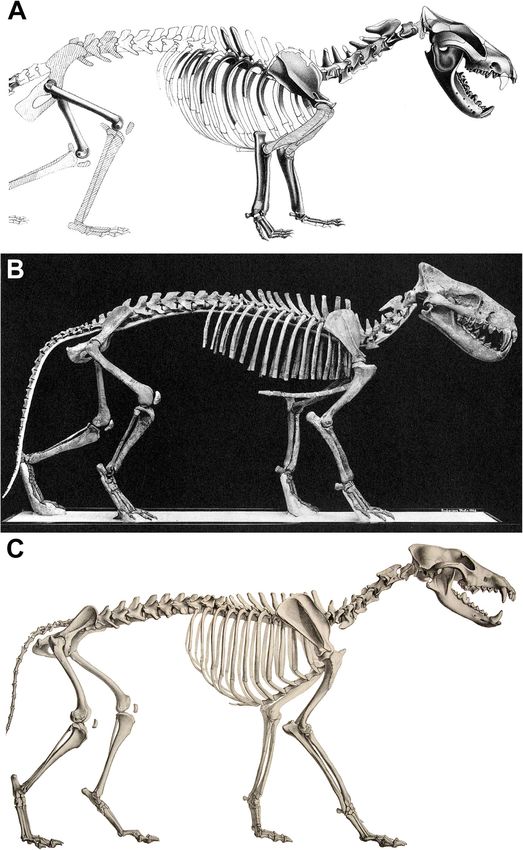
Fig. 7 Occipital region of a typical mammal (A; Procyon lotor, CMNH 22076), contrasting with the distinctive occiput morphology of lagomorphs
(B; Lepus sp., R. Engelman pers. col.), monotremes (C; Tachyglossus aculeata, CMNH 18877), and cingulates (D; Euphractus sexcinctus, R. Engelman
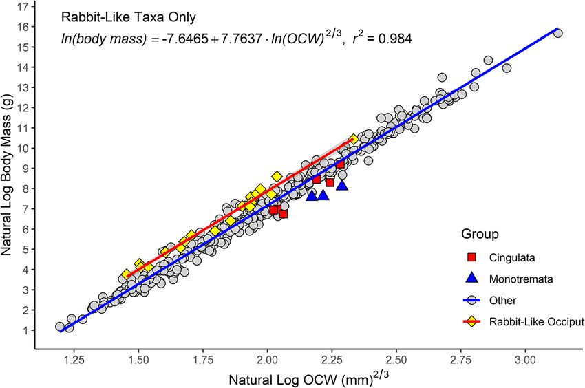
pers. col.). Scale = 1 cmEngelman BMC Biology (2022) 20:37 Page 14 of 44 the primary difference between these two groups driving Regression models by taxon the high residuals in taxa with rabbit-like condyles is a Datasets excluding taxa with apomorphic occiput shift in the y-intercept. This, in turn can be related to morphology (e.g., Monotremata, Lagomorpha) had lower the fact that the mediolaterally narrow condyles of lago- values of %PEcf and standard error of the estimate morphs and taxa with similar occiput morphology re- (%SEE), with %PEcf < 30% for all analyses (Table 4). Even sults in a lower OCW relative to other mammals. This when excluding these data, the regression line of the observation is further supported by the fact that the log-power model still showed a 2/3 power exponent slopes of the all-taxon regression line and a regression (Table 3). Calculating the regression line based only on line calculated based solely on with lagomorph-like oc- species with large sample sizes also resulted in lower cipital condyles are nearly identical (see Tables 4 and 6 error. However, the low error values for the equations and Fig. 8). A regression line could not be calculated for only including species with more than 10 observations Monotremata as only three monotreme taxa were in- may also be due to decreased taxonomic and morpho- cluded in this analysis and all extant monotremes span a logical breadth, as most species in these analyses pertain very narrow range of body sizes (2–3 kg). to a few taxonomic groups (Eulipotyphla, Rodentia, Car- Adding two additional binary categorical variables nivora) and only eight species in this analysis were larger to the model describing whether a taxon has a “lago- than 10 kg. The regression equation including only taxa morph-like” or “monotreme-like” occipital morph- for which body mass was greater than 1000 g produced ology results in higher r2 values and much lower %PE results that were almost identical to the regression for and %SEE (Table 6). The AIC (295), BIC (315), and the entire dataset (Table 4). log likelihood (− 143) for the model considering add- Examining the best-fit lines by order found that most itional variables for condyle shape are much lower species with sample sizes > 5 produced lines with similar than for any of the models only considering OCW allometries to the all species best-fit line, though some and body mass (compare these values to the ones re- groups had different intercept (Additional file 5). Testing ported in Table 2). Both the state of having of a for differences in intercept between mammalian orders monotreme-like occiput morphology (t = -5.702, p < (or suborders in the case of rodents) found non- 0.001) or a lagomorph-like occiput morphology (t = significant differences for the majority of clades (N = 19, 8.720, p < 0.001) significantly correlated with body Additional file 2). However, eight clades did show mass when considered as additional independent fac- significant differences in intercept: Castorimorpha, tor variables in the regression equation. Cingulata, Dermoptera, Lagomorpha, Macroscelidea, Fig. 8 Scatter plot of natural log of OCW raised to the 2/3 power against the natural log of body mass, showing groups that deviate from the main regression line (cingulates, monotremes, and taxa with rabbit-like occiputs) as well as the regression line formed by taxa with rabbit-like occiputs (in red)
Engelman BMC Biology    (2022) 20:37                                                                          Page 15 of 44

Monotremata, Paucituberculata, and Scandentia. These          to predict data beyond the upper and lower bounds of
clades are all groups which are either characterized by       the data (see Additional file 2). This can be seen in the
specialized occiput morphology relative to other mam-         very wide confidence intervals for the best-fit curve be-
mals (Castorimorpha, Cingulata, Dermoptera, Lago-             yond the distribution of measured species and the fact
morpha, Monotremata), or otherwise exhibit high               that the extrapolated curve for Australidelphia and Pri-
residuals as a clade (Macroscelidea, Scandentia, Paucitu-     mates did not follow the general shape of the data for all
berculata). Additionally, Macroscelidea, Scandentia, and      mammals. Perhaps the most extreme example of this
Paucituberculata exhibit higher p values (0.05 > p > 0.01)    was the all-Sciuromorph equation, which produced a
than taxa with extreme occiput specializations (p < 0.01).    concave-up curve with an extremely wide confidence
  Examining differences in slope between clades by cre-       interval. This result seems to be the result of several spe-
ating an interaction term between taxonomic group and         cies of Marmota spp., which are known to go through
OCW found that most of the differences between groups         extreme annual variation in body mass [136], but in this
were non-significant. When setting Artiodactyla as the        case the presence of a few species is able to massively in-
reference level (because of the low number of species in      fluence the shape of the loq-quadratic regression curve.
the alphabetically first taxon, Afrosoricida), the only       Indeed, for Sciuromorpha, the second-order term did
groups to have significantly different slopes were Afro-      not have a statistical effect (t = 1.054, p = 0.301).
soricida, Carnivora, Dasyuromorphia, Didelphimorphia,           Binning the data by superorder to increase sample size
and Hystricomorpha. However, the 95% confidence in-           results in regression curves for the five therian superor-
tervals for slopes all strongly overlap with one another      ders that are roughly comparable to the all-species
and the slope for the all-species regression line except      model. Xenarthra shows slightly more variation than
for Afrosoricida, which is composed of a small number         other therians, but this appears to be due to the low di-
of species spanning a narrow range of body sizes (N = 3,      versity within this clade and the presence of Cingulata
140–500 g), and thus this result might be due to sam-         (which exhibit specialized occiput morphology). When
pling error. Notably, the slope of Lagomorpha (which          comparing intercepts between superorders, Euarchonto-
are exclusively composed of species with a specialized        glires (t = 2.429, p = 0.0156) has a significantly different
occiput morphology) did not differ significantly from the     intercept from other therians, but this result appears to
remaining sample, further supporting the idea that resid-     be driven by the inclusion of species with a specialized
uals in the present equation are driven by differences in     lagomorph-like occiput (Lagomorpha, Caviidae) as in-
occiput shape rather than clade-specific patterns of allo-    cluding the presence of a lagomorph-like occiput as an
metric scaling.                                               additional explanatory variable reduces the statistical ef-
  Accuracy of the taxonomically restricted regression         fect of this result (t = 1.779, p = 0.073).
equations were higher than those of the total species re-       Overall, the results of the log-quadratic curves in this
gression, as would be expected based on previous stud-        study agree with the results of Campione [137] and
ies. The taxonomically narrowest dataset, the one             Müller et al. [138], who found that log-quadratic curves
including only sciuromorph rodents, produced the low-         were very unpredictable when extrapolated beyond the
est error values, suggesting that taxonomic breadth is        range of values used to calculate them and the detection
correlated with overall error rates. However, for the all-    of non-linear allometry was heavily dependent on the
rodent regression equation, residuals and %PEcf for ro-       range of body sizes included in the dataset, respectively.
dent taxa that were outliers in the total species regres-
sion (i.e., caviids, Dinomys, and Dipodomys) remain high      Phylogenetic signal and phylogenetic generalized least
even when rodents are considered by themselves. The           squares
QQ plot and histogram of the residuals of the rodent-         The residuals of the all-species regression equation show
only regression also show a strong departure from nor-        strong phylogenetic signal (mean λ = 0.901, p < 0.001).
mality (compare Fig. 5 and Additional file 6), suggesting     However, %PE and %SEE are much higher for under a
that all rodents may not conform to a single regression       Brownian model (%PE = 68.88%, %SEE = 276%) than
equation (though it is possible this departure from nor-      OLS (%PE = 32.03%, %SEE = 47.59) (Table 6). Applying
mality could disappear with a larger sample of rodents).      correction factors decreases this disparity (PGLS %PEcf,
Rodentia in general seems to show much higher vari-           31.56; OLS %PEcf, 31.09), but at the same time, PGLS re-
ation in occiput proportions than most other groups,          quires extremely large correction factors (1.754) that re-
even after accounting for the high diversity of this clade.   quire increasing the fitted value by over 75% to produce
  Under a log-quadratic model, the best-fit regression        a more accurate result, which suggests deeper methodo-
curve was somewhat more variable than the best-fit lines      logical problems that are being obscured by the use of
under a log-power model. In particular, the curvature of      correction factors. The high %SEE is likely due to the
the best-fit curve was not very well-resolved when trying     fact that PGLS does not remove the effects of phylogeny
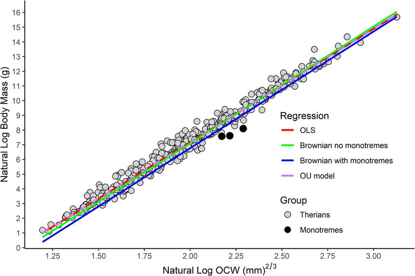
Engelman BMC Biology       (2022) 20:37                                                                                       Page 16 of 44

from the analysis nor adjust the predicted values based                selection. Indeed, it is rather concerning that whether or
on phylogenetic position, rather it merely fits the best-fit           not an OLS model is favored over a PGLS one is entirely
line that minimizes the covariance between the residuals               driven by relatively minor differences in tree choice.
of the regression and the underlying phylogenetic correl-              Notably, this variation in AIC and BIC did not correlate
ation matrix [139]. Indeed, PGLS generally results in                  with model prediction accuracy nor variation in model
higher standard errors, weaker correlations between var-               coefficients. That is, although PGLS under some trees
iables, and broader confidence intervals compared to                   produced an AIC lower than the OLS model, these
OLS [139].                                                             models did not produce more accurate results. Exclud-
   AIC, BIC, and log likelihood values for PGLS were ex-               ing one model that produced unusually poor support
tremely variable and depended entirely on which of the                 values, %PE ranged from 62.8 to 78.1% and %SEE ranged
trees from the random sample were chosen for analysis.                 from 219.9 to 452.6 across the 100 trees examined, at
Despite all 100 trees producing similar regression lines               minimum producing error statistics twice as high as
with a relatively little variation in the coefficients (slope          OLS. Because the goal of this study is predictive accur-
= 7.967 ± 0.088; y intercept = − 9.160 ± 0.179, see Add-               acy, rather than model fit, methods for PGLS as cur-
itional file 2), AIC and BIC values formed normal distri-              rently utilized are inappropriate here. Notably, the issues
butions with a range of over 150 and standard deviations               highlighted in this study are not driven by the data used,
of 50 (see Additional file 2), when differences of AIC                 but are broader issues concerning PGLS. As the focus of
more than 2 are considered statistically significant [140].            this paper is on using OCW as a body mass estimator,
However, the mean and median values for both AIC                       addressing these issues is beyond the scope of the paper.
(mean = 406, median = 396) and BIC (mean = 418, me-                      The PGLS model under Brownian motion produced a
dian = 408) were higher than for OLS. This extreme                     best-fit line that almost completely bypassed the distri-
variability in AIC values is noteworthy given that all of              bution of the data (Fig. 9). This pattern is almost entirely
the PGLS analyses used the same dataset, the trees were                driven by the apomorphic occiput of Monotremata (see
similar enough in topology for each to be considered a                 “Discussion”), demonstrated by the fact that omitting
reasonable approximation of mammalian phylogeny, and                   monotremes results in a regression line very close to
the resulting regression equations were near-identical.                that produced by an OLS or OU model. Even excluding
The high variability in AIC, BIC, and log likelihood                   Monotremata phylogenetic signal in the dataset was still
values in potential most parsimonious trees makes it al-               very high (mean λ = 0.884, p < 0.001), the resulting
most impossible to use these statistics to make model                  goodness-of-fit and the accuracy of PGLS (%PE = 36.12,

 Fig. 9 Linear regression between log OCW and log body mass under OLS (in red), PGLS under a Brownian model (in blue), PGLS under a
 Brownian model excluding monotremes (in green), and PGLS under an OU model (in purple, dashed to not obscure the other lines), showing
 how the inclusion of monotreme taxa greatly biases the PGLS regression line under a Brownian model due to the deep divergence between
 Theria and Monotremata
You can also read