OECD Environmental Outlook to 2050 - Climate Change Chapter PRE-RELEASE VERSION
←
→
Page content transcription
If your browser does not render page correctly, please read the page content below

OECD Environmental Outlook to 2050
                                         Climate Change Chapter

                                         PRE-RELEASE VERSION

www.oecd.org/environment/outlookto2050                             November 2011
OECD ENVIRONMENTAL OUTLOOK TO 2050

              CHAPTER 3: CLIMATE CHANGE

                 PRE-RELEASE VERSION, NOVEMBER 2011

The OECD Environmental Outlook to 2050 was prepared by a joint team from the OECD Environment
      Directorate (ENV) and the PBL Netherlands Environmental Assessment Agency (PBL).

                                            Authors:
                Virginie Marchal, Rob Dellink (ENV) Detlef van Vuuren (PBL)
                Christa Clapp, Jean Château, Eliza Lanzi, Bertrand Magné (ENV)
                                     Jasper van Vliet (PBL)

                                           Contacts:
                         Virginie Marchal (virginie.marchal@oecd.org)
                              Rob Dellink (rob.dellink@oecd.org)

                                              1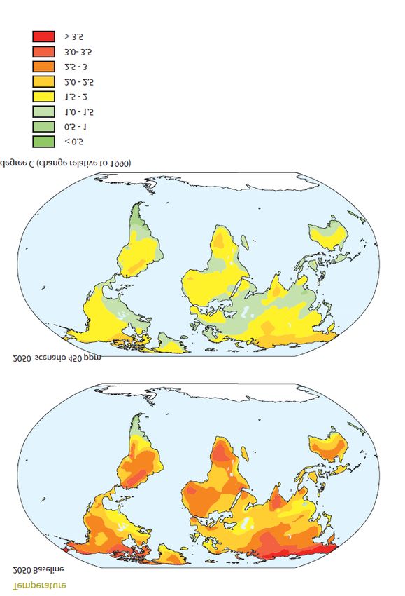
TABLE OF CONTENTS

   Key messages ...............................................................................................................................................5
     Trends and projections .............................................................................................................................5
     Policy steps to build a low-carbon, climate-resilient economy ................................................................6
   3.1. Introduction .......................................................................................................................................9
   3.2. Trends and projections ......................................................................................................................9
     Greenhouse gas emissions and concentrations .........................................................................................9
     Impacts of climate change ......................................................................................................................17
   3.3. Climate Change: The state of policy today .....................................................................................23
     The international challenge: Overcoming inertia ...................................................................................23
     National action to mitigate climate change ............................................................................................24
     National action to adapt to climate change.............................................................................................38
     Getting the policy mix right: Interactions between adaptation and mitigation ......................................42
   3.4. Policy steps for tomorrow: Building a low-carbon, climate-resilient economy..............................43
     What if …? Three scenarios for stabilising emissions at 450 ppm ........................................................43
     Less stringent climate mitigation (550 ppm) scenarios ..........................................................................62
     Actions needed for an ambitious, global climate policy framework ......................................................63
     Finding synergies among climate change strategies and other goals .....................................................66
NOTES ..........................................................................................................................................................71
REFERENCES ..............................................................................................................................................75
ANNEX 3.A1: MODELLING BACKGROUND INFORMATION ON CLIMATE CHANGE .................83
   The Baseline scenario ................................................................................................................................83
   The 450 ppm climate stabilisation scenarios .............................................................................................84
     Alternative permit allocation schemes ...................................................................................................84
     Technology options in the 450 ppm scenario.........................................................................................85
     Cancún Agreements/Copenhagen Accord pledges ................................................................................86
     Phasing out fossil fuel subsidies.............................................................................................................88
ANNEX NOTES ...........................................................................................................................................89

Tables

   Table 3.1. Examples of policy tools for climate change mitigation .......................................................25
   Table 3.2. National climate change legislation: Coverage and scope, selected countries ......................27
   Table 3.3. Status of emission trading schemes .......................................................................................29
   Table 3.4. Adaptation options and potential policy instruments ............................................................39
   Table 3.5. Overview of the Environmental Outlook mitigation scenarios .............................................44
   Table 3.6. How targets and actions pledged under the Copenhagen Accord and Cancún Agreements
   are interpreted as emission changes under the 450 Delayed Action scenario: 2020 compared to 1990 ....57
   Table.3.7 How different factors will affect emissions and real income from the Cancún
   Agreements/Copenhagen Accord pledges: 450 Delayed Action scenario) ................................................59

                                                                                2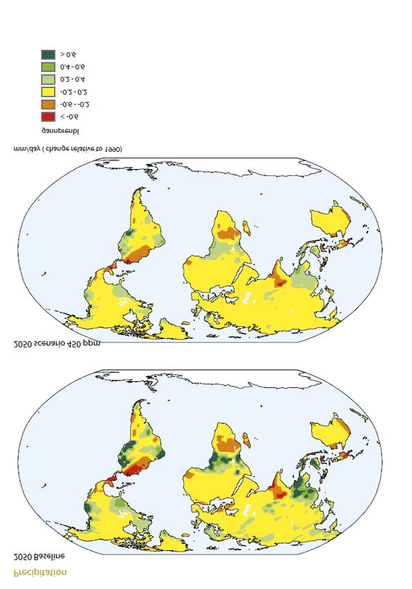
Table.3.8. Competitiveness impacts of the 450 Delayed Action scenario, 2020 and 2050: % change
 from Baseline .............................................................................................................................................61
 Table 3.9. Income impacts of a fossil fuel subsidy reform with and without the 450 Core scenario,
 2020 and 2050: % real income deviation from the Baseline .....................................................................66
 Table 3.10.    Economic impact of an OECD-wide emissions trading scheme where labour markets are
 rigid, assuming lump-sum redistribution, 2015-2030: % deviation from the business-as-usual scenario .70
 Table 3.11.    Economic impact of an OECD-wide ETS for different recycling options, assuming
 medium labour market rigidity, 2015-2030 ...............................................................................................70

Figures

 Figure 3.1.     GHG emissions: Baseline, 1970-2005...............................................................................10
 Figure 3.2.. Decoupling trends: CO2 emissions versus GDP in the OECD and BRIICS, 1990-2010 ..11
 Figure 3.3.     Energy related CO2 emission per capita, OECD/ BRIICS, 2000 and 2008 .......................12
 Figure 3.4.     Change in production-based and demand-based CO2 emissions: 1995-2005 ...................13
 Figure 3.5.     GHG emissions to 2050; Baseline, 2010-2050..................................................................14
 Figure 3.6.     GHG emissions per capita: Baseline, 2010-2050 ..............................................................14
 Figure 3.7.     Global CO2 emissions by source: Baseline, 1980-2050.....................................................15
 Figure 3.8.     CO2 emissions from land use: Baseline, 1990-2050 ..........................................................16
 Figure 3.9.     Long-run CO2-concentrations and temperature increase; Baseline1970-2100 ..................17
 Figure 3.10. Change in annual temperature: Baseline and 450oppm scenarios, 1990-2050 ..................18
 Figure 3.11. Change in annual precipitation: Baseline, 1990-2050 .......................................................19
 Figure 3.12. Key impacts of increasing global temperature ..................................................................20
 Figure 3.13. Assets exposed to sea-level rise in coastal cities by 2070 .................................................22
 Figure 3.14 Government RD&D expenditures in energy in IEA member countries: 1974-2009.........34
 Figure 3.15. New plant entry by type of renewable energy in North America, Pacific and EU-15
 regions, 1978-2008 ....................................................................................................................................35
 Figure 3.16. Alternative emission pathways, 2010-2100 .......................................................................45
 Figure 3.17. Concentration pathways for the four Outlook scenarios including all climate forcers,
 2010-2100       47
 Figure 3.18. 450oCore Scenario: emissions and cost of mitigation, 2010-2050 ....................................48
 Figure 3.19. Impact of permit allocation schemes on emission allowances and real income in 2050...51
 Figure 3.20. GHG abatements in the 450 Core Accelarated Action and 450 Core scenarios compared
 to the Baseline, 2020 and 2030 ..................................................................................................................53
 Figure 3.21. Technology choices for the 450 Accelerated Action scenario ...........................................55
 Figure.3.22. Regional real income impacts: 450 Core versus 450 Delayed Action scenarios ...............58
 Figure.3.23. Change in global GHG emissions in 2050 compared to 2010: 450 Delayed Action and
 550oppm scenarios .....................................................................................................................................62
 Figure 3.24.      Change in real income from the Baseline for the 450 Delayed Action and 550 Core
 scenarios, 2050 63
 Figure 3.25. Income impact of fragmented emission trading schemes for reaching concentrations of
 550oppm compared to the Baseline, 2050 ..................................................................................................64
 Figure.3.26. Impact on GHG emissions of phasing out fossil fuels subsidies, 2050 .............................65
 Figure 3.A1. Permit allocation schemes, 2020 and 2050........................................................................85
 Figure 3.A2. Nuclear installed capacity in the Progressive nuclear phase out scenario, 2010-2050.....86

Boxes

 Box 3.1.           Production versus demand-based emissions..........................................................................13
 Box 3.2.           Land-use emissions of CO2 – past trends and future projections ..........................................16
 Box 3.3.           Example of assets exposed to climate change: Coastal cities................................................22

                                                                            3
Box 3.4. The EU-Emissions Trading Scheme: Recent developments .................................................30
Box 3.5. The growth in renewable energy power plants ......................................................................35
Box 3.6. Greening household behaviour: The role of public policies ..................................................37
Box 3.7. The UNEP Emissions Gap report ..........................................................................................46
Box 3.8. Cost uncertainties and modelling frameworks ......................................................................49
Box 3.9. What if…the mitigation burden was shared differently? How permit allocation rules matter50
Box 3.10. Implications of technology options .......................................................................................54
Box 3.11. Mind the gap: Will the Copenhagen pledges deliver enough? ..............................................59
Box 3.12. What if... a global carbon market does not emerge? .........................................................64
Box 3.13. Bioenergy: Panacea or Pandora’s Box? ....................................................................................67
Box 3.14. The case of black carbon .......................................................................................................68
Box 3.15. What if…reducing GHGs could increase employment? .......................................................69
4Key messages
Climate change presents a global systemic risk to society. It threatens the basic elements of life for
all people: access to water, food production, health, use of land, and physical and natural capital.
Inadequate attention to climate change could have significant social consequences for human well-being,
hamper economic growth and heighten the risk of abrupt and large-scale changes to our climatic and
ecological systems. The significant economic damage could equate to a permanent loss in average per-
capita world consumption of more than 14% (Stern, 2006). Some poor countries would be likely to suffer
particularly severely. This chapter demonstrates how avoiding these economic, social and environmental
costs will require effective policies to shift economies onto low-carbon and climate-resilient growth paths.
Trends and projections
Environmental state and pressures
• RED Global greenhouse gas (GHG) emissions continue to increase, and in 2010 global
energy-related carbon-dioxide (CO2) emissions reached an all-time high of 30.6 gigatonnes
(Gt) despite the recent economic crisis. The Environmental Outlook Baseline scenario envisages
that without more ambitious policies than those in force today, GHG emissions will increase by
another 50% by 2050, primarily driven by a projected 70% growth in CO2 emissions from energy
use. This is primarily due to a projected 80% increase in global energy demand. Transport
emissions are projected to double, due to a strong increase in demand for cars in developing
countries. Historically, OECD economies have been responsible for most of the emissions. In the
coming decades, increasing emissions will also be caused by high economic growth in some of
the major emerging economies.
GHG emissions by region: Baseline, scenario 2010-2050
Note: “OECD AI” stands for the group of OECD countries that are also part of Annex I of the Kyoto Protocol.
GtCO2e = Gigatonnes of CO2 equivalent.
Source: OECD Environmental Outlook Baseline; output from ENV-Linkages.
5• RED Without more ambitious policies, the Baseline projects that atmospheric concentration of
GHG would reach almost 685 parts per million (ppm) CO2-equivalents by 2050. This is well
above the concentration level of 450 ppm required to have at least a 50% chance of stabilising the
climate at a 2-degree (2 °C) global average temperature increase, the goal set at the 2010
United Nations Framework Convention on Climate Change (UNFCCC) Conference in Cancún.
Under the Baseline projection, global average temperature is likely to exceed this goal by 2050,
and by 3 °C to 6 °C higher than pre-industrial levels by the end of the century. Such a high
temperature increase would continue to alter precipitation patterns, melt glaciers, cause sea-level
rise and intensify extreme weather events to unprecedented levels. It might also exceed some
critical “tipping-points”, causing dramatic natural changes that could have catastrophic or
irreversible outcomes for natural systems and society.
• YELLOW Technological progress and structural shifts in the composition of growth are
projected to improve the energy intensity of economies in the coming decades (i.e. achieving a
relative decoupling of GHG emissions growth and GDP growth), especially in OECD and the
emerging economies of Brazil, Russia, India, Indonesia, China and South Africa (BRIICS).
However, under current trends, these regional improvements would be outstripped by the
increased energy demand worldwide.
• YELLOW Emissions from land use, land-use change and forestry (LULUCF) are projected to
decrease in the course of the next 30 years, while carbon sequestration by forests increases. By
2045, net-CO2 emissions from land use are projected to become negative in OECD countries.
Most emerging economies also show a decreasing trend in emissions from an expected slowing
of deforestation. In the rest of the world (RoW), land-use emissions are projected to increase to
2050, driven by expanding agricultural areas, particularly in Africa.
Policy responses
• RED Pledging action to achieve national GHG emission reduction targets and actions under the
UNFCCC at Copenhagen and Cancún was an important first step by countries in finding a global
solution. However, the mitigation actions pledged by countries are not enough to be on a least-
cost pathway to meet the 2 °C goal. Limiting temperature increase to 2 °C from these pledges
would require substantial additional costs after 2020 to ensure that atmospheric concentrations of
GHGs do not exceed 450 ppm over the long term. More ambitious action is therefore needed now
and post-2020. For example, 80% of the projected emissions from the power sector in 2020 are
inevitable, as they come from power plants that are already in place or are being built today. The
world is locking itself into high carbon systems more strongly every year. Prematurely closing
plants or retrofitting with carbon capture and storage (CCS) – at significant economic cost, –
would be the only way to reverse this “lock-in”.
• YELLOW Progress has been made in developing national strategies for adapting to climate
change. These also encourage the assessment and management of climate risk in relevant sectors.
However, there is still a long way to go before the right instruments and institutions are in place
to explicitly incorporate climate change risk into policies and projects, increase private-sector
engagement in adaptation actions and integrate climate change adaptation into development co-
operation.
Policy steps to build a low-carbon, climate-resilient economy
We must act now to reverse emission trends in order to stabilise GHG concentrations at 450 ppm
CO2e and increase the chance of limiting the global average temperature increase to 2 °C. Ambitious
6mitigation action substantially lowers the risk of catastrophic climate change. The cost of reaching the 2 °C
goal would slow global GDP growth from 3.5 to 3.3% per year (or by 0.2 percentage-points) on average,
costing roughly 5.5% of global GDP in 2050. This cost should be compared with the potential cost of
inaction that could be as high as 14% of average world consumption per capita according to some
estimates (Stern, 2006).
Delaying action is costly. Delayed or only moderate action up to 2020 (such as implementing the
Copenhagen/Cancún pledges only, or waiting for better technologies to come on stream) would increase
the pace and scale of efforts needed after 2020. It would lead to 50% higher costs in 2050 compared to
timely action, and potentially entail higher environmental risk.
A prudent response to climate change calls for both an ambitious mitigation policy to reduce further
climate change, and timely adaptation policies to limit damage from the impacts that are already inevitable.
In the context of tight government budgets, finding least-cost solutions and engaging the private sector will
be critical to finance the transition. Costly overlaps between policies must also be avoided. The following
actions are a priority:
• Adapt to inevitable climate change. The level of GHG already in the atmosphere means that some
changes in the climate are now inevitable. The impact on people and ecosystems will depend on how
the world adapts to those changes. Adaptation policies will need to be implemented to safeguard the
well-being of current and future generations worldwide.
• Integrate adaptation into development co-operation. The management of climate change risks is
closely intertwined with economic development – impacts will be felt more by the poorest and most
vulnerable populations. National governments and donor agencies have a key role to play and
integrating climate change adaptation strategies into all development planning is now critical. This
will involve assessing climate risks and opportunities within national government processes, at
sectoral and project levels, and in both urban and rural contexts. The uncertainty surrounding climate
impacts means that flexibility is important.
• Set clear, credible, more stringent and economy-wide GHG-mitigation targets to guide policy and
investment decisions. Participation of all major emission sources, sectors and countries would reduce
the costs of mitigation, help to address potential leakage and competitiveness concerns and could even
out ambition levels for mitigation across countries.
• Put a price on carbon. This Outlook models a 450 ppm Core scenario which suggests that achieving
the 2 °C goal would require establishing clear carbon prices that are increased over time. This could be
done using market-based instruments like carbon taxes or emission trading schemes. These can
provide a dynamic incentive for innovation, technological change and driving private finance towards
low-carbon, climate-resilient investments. These can also generate revenues to ease tight government
budgets and potentially provide new sources of public funds. For example, if the Copenhagen Accord
pledges and actions for Annex I countries were to be implemented as a carbon tax or a cap-and-trade
scheme with fully auctioned permits, in 2020 the fiscal revenues would amount to more than
USD 250 billion, i.e 0.6% of their GDP.
• Reform fossil fuel support policies. Support to fossil fuel production and use in OECD countries is
estimated to have been about USD 45-75 billion a year in recent years; developing and emerging
economies provided USD 409 billion in 2010 (IEA data). OECD Outlook simulation shows that
phasing out fossil fuels subsidies in developing countries could reduce by 6% global energy-related
GHG emissions, provide incentives for increased energy efficiency and renewable energy and also
increase public finance for climate action. However, fossil fuel subsidy reforms should be
7implemented carefully while addressing potential negative impacts on households through appropriate
measures.
• Foster innovation and support new clean technologies. The cost of mitigation could be significantly
reduced if R&D could come up with new breakthrough technologies. For example, emerging
technologies – such as bioenergy from waste biomass and CCS – have the potential to absorb carbon
from the atmosphere. Perfecting these technologies, and finding new ones, will require a clear price on
carbon, targeted government-funded R&D, and policies to reduce the financial risks of investing in
new low-carbon technologies and to boost their deployment.
• Complement carbon pricing with well-designed regulations. Carbon pricing and support for
innovation may not be enough to ensure all energy-efficiency options are adopted or accessible.
Additional targeted regulatory instruments (such as fuel, vehicle and building-efficiency standards)
may also be required. If designed to overcome market barriers and avoid costly overlap with market-
based instruments, they can accelerate the uptake of clean technologies, encourage innovation and
reduce emissions cost-effectively. The net contribution of the instrument “mix” to social welfare,
environmental effectiveness and economic efficiency should be regularly reviewed.
83.1. Introduction
Climate change is a serious global systemic risk that threatens life and the economy. Observations of
increases in global average temperatures, widespread melting of snow and ice, and a rising global average
sea level indicate that the climate is already warming (IPCC, 2007a). If greenhouse gas (GHG) emissions
continue to grow, this could result in a wide range of adverse impacts and potentially trigger large-scale,
irreversible and catastrophic changes (IPCC, 2007b) that will exceed the adaptive capacity of natural and
social systems. The environmental, social and economic costs of inaction are likely to be significant.
Agreements reached in Cancún, Mexico, at the 2010 United Nations Climate Change Conference
recognised the need for deep cuts in global GHG emissions in order to limit the global average temperature
increase to 2 degrees Celsius (2 °C) above pre-industrial levels (UNFCCC, 2011a). A temperature increase
of more than 2 °C is likely to push components of the Earth’s climate system past critical thresholds, or
“tipping points” (EEA, 2010).
This chapter seeks to analyse the policy implications of the climate change challenge. Are current
emission reduction pledges enough to stabilise climate change and limit global average temperature
increase to 2 °C? If not, what will the consequences be? What alternative growth pathways could achieve
this goal? What policies are needed, and what will be the costs and benefits to the economy? And last, but
not least, how can the world adapt to the changes that are already occurring?
To shed light on these questions, this chapter first looks at the “business-as-usual” situation, using
projections from the Environmental Outlook Baseline scenario, to see what the climate would be like in
2050 if no new action is taken. 1 It then compares different policy scenarios against this “no-new-policy”
Baseline scenario to understand how the situation could be improved. Section 3.3 (“Climate Change: The
state of policy today”) describes how a prudent response to climate change involves a two-pronged
approach: ambitious mitigation policies 2 to reduce further climate change, as well as timely adaptation3
policies to limit damage by climate change impacts that are inevitable. Mitigation and adaptation policies
are essential, and they are complementary. Most countries have begun to respond through actions at the
international, national and local levels, drawing on a mix of policy instruments that include carbon pricing,
other energy-efficiency policies, information-based approaches and innovation. Some progress can be
noted, but much more needs to be done to achieve the 2 °C goal.
The chapter concludes by outlining how limiting global warming will require transformative policies
to reconcile short-term action with long-term climate objectives, balancing their costs and benefits. The
transition to a low-carbon, climate-resilient development path requires financing, innovation and strategies
that also address potential negative competitiveness and employment impacts. Such a path can also create
new opportunities as part of a green growth strategy. Thus, the work presented here shows that through
appropriate policies and international co-operation, climate change can be tackled in a way that will not
cap countries’ aspirations for growth and prosperity.
3.2. Trends and projections
Greenhouse gas emissions and concentrations
Historical and recent trends
Several gases contribute to climate change. The Kyoto Protocol 4 intends to limit emissions of the six
gases which are responsible for the bulk of global warming. Of these, the three most potent are carbon
dioxide (CO2), methane (CH4), and nitrous oxide (N2O), currently accounting for 98% of the GHG
emissions covered by the Kyoto Protocol (Figure 3.1). The other gases, hydrofluorocarbons (HFCs),
perfluorocarbons (PFCs) and sulphur hexafluoride (SF6) account for less than 2%, but their total emissions
9are growing. These gases differ in terms of their warming effect and their longevity in the atmosphere.
Apart from these six GHGs, there are several other atmospheric substances that lead to warming
(e.g. chlorofluorocarbons or CFCs, and black carbon – see Box 3.14) or to cooling (e.g. sulphate aerosols).
Unless otherwise mentioned, in this chapter the term “emissions” refers to the Kyoto gases only, while the
climate impacts described are based on a consideration of all the climate forcing gases (the term “climate
forcer” is used for any gas or particle that alters the Earth’s energy balance by absorbing or reflecting
radiation).
Global GHG emissions have doubled since the early 1970s (Figure 3.1), driven mainly by economic
growth and increasing fossil-energy use in developing countries. Historically, OECD countries emitted the
bulk of GHG emissions, but the share of Brazil, Russia, India, Indonesia, China and South Africa (the
BRIICS countries) in global GHG emissions has increased to 40%, from 30% in the 1970s.
Overall, the global average concentrations of various GHGs in the atmosphere have been
continuously increasing since records began. In 2008, the concentration of all GHGs regulated in the Kyoto
Protocol was 438 parts per million (ppm) CO2-equivalent (CO2e). This was 58% higher than the pre-
industrial level (EEA, 2010a). It is coming very close to the 450 ppm threshold, the level associated with a
50% chance of exceeding of the 2 °C global average temperature change goal (see Section 3.4).
Figure 3.1. GHG emissions: Baseline, 1970-2005
By regions By gases
OECD BRIICS ROW CO2
CO2 CH4
CH4 N2O
N2O HFC,PFCs
HFC, PFCs& &SF6
SF6
50
50
GtCO2e
GtCO2e
45 45
40 40
35 35
30 30
25 25
20 20
15 15
10 10
5 5
0 0
1970 1975 1980 1985 1990 1995 2000 2005 1970 1975 1980 1985 1990 1995 2000 2005
Note: BRIICS excludes the Republic of South Africa which is aggregated in the rest of the world (RoW) category. The emissions of
fluor gases are not included in the totals by region.
Source: OECD Environmental Outlook Baseline; output from IMAGE.
Carbon-dioxide emissions
Today CO2 emissions account for around 75% of global GHG emissions. While global CO2 emissions
decreased in 2009 – by 1.5% – due to the economic slowdown, trends varied depending on the country
context: developing countries (non-Annex I, see Section 3.3) emissions continued to grow by 3%, led by
China and India, while emissions from developed countries fell sharply – by 6.5% (IEA, 2011a). Most CO2
emissions come from energy production, with fossil fuel combustion representing two-thirds of global CO2
emissions. Indications of trends for 2010 suggest that energy-related CO2 emissions will rebound to reach
their highest ever level at 30.6 gigatonnes (GtCO2), a 5% increase from the previous record year of 2008. 5
10A slow-down in OECD emissions has been more than compensated for by increased emissions in non-
OECD countries, mainly China – the country with the largest energy-related GHG emissions since 2007
(IEA, 2011a).
In 2009, CO2 emissions originated from fossil fuel combustions were based on coal (43%), followed
by oil (37%) and gas (20%). Today’s rapid economic growth, especially in the BRIICS, is largely
dependent on increased use of carbon-intensive coal-fired power, driven by the existence of large coal
reserves with limited reserves of other energy sources. While emission intensities in economic terms
(defined as the ratio of energy use to GDP) vary greatly around the world, CO2 emissions are growing at a
slower rate than GDP in most OECD and emerging economies (Figure 3.2). In other words, CO2 emissions
are becoming relatively “decoupled” from economic growth.
Figure 3.2. Decoupling trends: CO2 emissions versus GDP in the OECD and BRIICS, 1990-2010
a. OECD b. BRIICS
350 350
CO2
CO2 emissions f rom production CO2
CO emissions ffrom
2 emissions rom production
production
300 Real GDP 300 Real GDP
Real net national disposable income Gross National Income
250 250
Index 1990=100
Index 1990=100
200 200
150 150
100 100
50 50
0 0
1990 1994 1998 2002 2006 2010 1990 1994 1998 2002 2006 2010
Note: CO2 data refer to emissions from energy use (fossil fuel combustion).
Source: Adapted from OECD (2011e), Towards Green Growth: Monitoring Progress, OECD Green Growth Studies, OECD, Paris,
based on OECD, IEA and UNFCCC data.
On a per-capita basis, OECD countries still emit far more CO2 than most other world regions, with
10.6 tonnes of CO2 emitted per capita on average in OECD countries in 2008, compared with 4.9 tonnes in
China, and 1.2 tonnes in India (Figure 3.3). However, rapidly expanding economies are significantly
increasing their emissions per capita. China for instance doubled its emissions per capita between 2000 and
2008. These calculations are based on the usual definition that emissions are attributed to the place where
they occur, sometimes labelled the “production-based emissions accounting approach”. If one allocates
emissions according to their end-use, i.e. using a consumption-based approach, part of the emission
increases in the BRIICS regions would be attributed to the OECD countries, as these emissions are
“embedded” in exports from the BRIICS to the OECD (see Box 3.1).
11Figure 3.3. Energy-related CO2 emissions per capita, OECD/ BRIICS: 2000 and 2008
25
tonnes of CO2 per capita
2008
20
2000
15
10
5
0 Denmark
Netherlands
Hungary
Germany
Luxembourg
Chile
Sweden
Slovakia
Poland
Finland
China
Czech Republic
Turkey
Mexico
Switzerland
Norway
Slovenia
Estonia
Canada
India
Brazil
Indonesia
Russian Federation
OECD
Portugal
Iceland
Spain
Ireland
Belgium
Australia
New Zealand
Japan
United Kingdom
France
Italy
Greece
Austria
Israel
South Africa
Korea, Republic of
United States
Note: Production-based emissions, in tonnes of CO2 per capita.
Source: Based on OECD (2011e), Towards Green Growth: Monitoring Progress, OECD Green Growth Studies, from IEA data.
Other gases
Methane is the second largest contributor to human-induced global warming, and is 25 times more
potent than CO2 over a 100-year period. Methane emissions contribute to over one-third of today’s human-
induced warming. As a short-lived climate forcer, limiting methane emissions will be a critical strategy for
reducing the near-term rate of global warming and avoiding exceeding climatic tipping points (see below).
Methane is emitted from both anthropogenic and natural sources; over 50% of global methane emissions
are from human activities 6, such as fossil fuel production, animal husbandry (enteric fermentation in
livestock and manure management), rice cultivation, biomass burning and waste management. Natural
sources of methane include wetlands, gas hydrates, permafrost, termites, oceans, freshwater bodies, non-
wetland soils, and other sources such as wildfires.
Nitrous oxide (N2O) lasts a long time in the atmosphere (approximately 120 years) and has powerful
heat trapping effects – about 310 times more powerful than CO2. It therefore has a large global warming
potential. Around 40% of N2O emissions are anthropogenic, and come mainly from soil management,
mobile and stationary combustion of fossil fuel, adipic acid production (used in the production of nylon),
and nitric acid production (for fertilisers and the mining industry).
CFCs and HCFCs are powerful GHGs that are purely man-made and used in a variety of applications.
As they also deplete the ozone layer, they have been progressively phased out under the Montreal Protocol
on Substances That Deplete the Ozone Layer. HFCs and PFCs are being used as replacements for CFCs.
While their contribution to global warming is still relatively small, it is growing rapidly. They are produced
from chemical processes involved in the production of metals, refrigeration, foam blowing and
semiconductor manufacturing.
12Box 3.1. Production versus demand-based emissions
Production-based accounting of CO2 emissions allocates emissions to the country where production occurs – it
does not account for emissions caused by final domestic demand. Alternatively, consumption-based accounting
differs from traditional, production-based inventories because of imports and exports of goods and services that,
either directly or indirectly, involve CO2 emissions. Emissions embedded in imported goods are added to direct
emissions from domestic production, while emissions related to exported goods are deducted. A comparison
between the two approaches shows that total emissions generated to meet demand in OECD countries have
increased faster than emissions from production in these countries (Figure 3.4).
However, international comparisons should be interpreted with caution as country differences are due to a host
of factors – including climate change mitigation efforts, trends in international specialisation, and countries’ relative
competitive advantages. While the fast growth of production-based emissions in the BRIICS may partly reflect the
worldwide shift of heavy industry and manufacturing to emerging economies, these figures should not be confused
with carbon leakage* effects as they are based on observed trends in production, consumption and trade patterns.
Figure 3.4. Change in production-based and demand-based CO2 emissions: 1995-2005
Panel A. Average annual rate of change, 1995-2005 Panel B. Trade balance (production-consumption) in
CO2 emissions as % of global CO2 emissions
OECD BRIICS OECD BRIICS
4% 8%
Average annual rate of change, 1995-2005
6% 7.0%
3.8%
% of global CO2 emissions
4% 5.0% 5.2%
3% 3.3%
2%
0%
2%
-2%
1.6%
-4% -4.9%
1%
1.1% -6.1%
-6%
-7.3%
-8%
0% 1995 2000 2005
Demand-based CO
Demand-based CO2
2 Production-based CO2
CO2
Source: OECD (2011e), Towards Green Growth: Monitoring Progress, OECD Green Growth Studies, based on IEA data.
Note: *Carbon leakage occurs when a mitigation policy in one country leads to increased emissions in other countries, thereby
eroding the overall environmental effectiveness of the policy. Leakage can occur through a shift in economic activity towards
unregulated countries, or through increased fossil-energy use induced by lower pre-tax fuel prices resulting from the mitigation
action.
Future emission projections
This section presents the key findings of the Environmental Outlook Baseline scenario, which looks
forward to 2050 and is based on business as usual in terms of policies and on the socio-economic
projections described in Chapter 2 (see Annex 3.A1 for more detail on the assumptions underlying the
Baseline). Any projection of future emissions is subject to fundamentally uncertain factors, such as
demographic growth, productivity gains, fossil fuels prices and energy efficiency gains. The scenario
suggests that GHG emissions will continue to grow to 2050. Despite sizeable energy-efficiency gains,
energy and industry-related emissions are projected to more than double to 2050 compared to 1990 levels.
Meanwhile, net emissions from land-use change are projected to decrease rapidly (Box 3.2). Emissions
from BRIICS countries are projected to account for most of the increase (Figure 3.5). This is driven by
growth in population and GDP per capita, leading to growing per-capita GHG emissions. In the OECD,
emissions are projected to grow at a slower pace, partly reflecting demographic decline and slower
13economic growth, as well as existing climate policies. Overall, the contribution of OECD countries to
global GHG emissions is projected to drop to 23%, but OECD countries will continue to have the highest
emissions per capita (Figure 3.6).
Figure 3.5. GHG emissions: Baseline, 2010-2050
a. By gases b. By regions
CO2 (energy+industrial) CO2 (Land use) CH4 N2O HFC+PFC+SF6 OECD A1 (23% in 2050) Russia & rest of A1(7%)
Rest of BRIICS (44%) ROW (26%)
90 90
GtCO2e
GtCO2e
80 80
70 70
60 60
50 50
40 40
30 30
20 20
10 10
0 0
2010
2012
2014
2016
2018
2020
2022
2024
2026
2028
2030
2032
2034
2036
2038
2040
2042
2044
2046
2048
2050
2010
2012
2014
2016
2018
2020
2022
2024
2026
2028
2030
2032
2034
2036
2038
2040
2042
2044
2046
2048
2050
Source: OECD Environmental Outlook Baseline; output from IMAGE/ENV Linkages.
Figure 3.6. GHG emissions per capita: Baseline, 2010-2050
2010 2020 2050
16 15.3
14 13.4
tCO2 / per capita
12
10.4
10 8.9
8
6.2
6 5.4 5.5
3.8
4
2
0
OECD BRIICS ROW World
Source: OECD Environmental Outlook Baseline; output from IMAGE/ENV-Linkages.
Carbon-dioxide emissions
CO2 emissions are projected to remain the largest contributor to global GHG emissions, driven by
economic growth based on fossil fuel use in the energy and industrial sectors. The International Energy
14Agency (IEA) estimates that unless policies prematurely close existing facilities, 80% of projected 2020
emissions from the power sector are already locked in, as they will come from power plants that are
currently in place or under construction (IEA, 2011b). Under the Environmental Outlook Baseline, demand
for energy is projected to increase by 80% between 2010 and 2050. Transport emissions are projected to
double between 2010 and 2050, due in part to a strong increase in demand for cars in developing countries,
and growth in aviation (Figure 3.7). However, CO2 emissions from land use, land-use change and forestry
(LULUCF), driven in the last 20 years by the rapid conversion of forests to grassland and cropland in
tropical regions, are expected to decline over time and even become a net sink of emissions in the 2040-
2050 timeframe in OECD countries (Figure 3.5 and 3.8 and Box 3.2).
Figure 3.7. Global CO2 emissions by source: Baseline, 1980-2050
60
Industrial
GtCO2
processes
50 Power
generation
Energy
40 transf ormation*
Transport
30
Industry
20 Residential
Services
10
Other sectors
0
1980 1990 2000 2010 2020 2030 2040 2050
Note: The category “energy transformation” includes emissions from oil refineries, coal and gas liquefaction.
Source: OECD Environmental Outlook Baseline; output from IMAGE.
Other gases
Methane and nitrous oxide emissions are projected to increase to 2050. Although agricultural land is
expected to expand only slowly, the intensification of agricultural practices (especially the use of
fertilisers) in developing countries and the change of dietary patterns (increasing consumption of meat) are
projected to drive up these emissions. At the same time, emissions of HFCs and PFCs, driven by increasing
demand for coolants and use in semiconductor manufacturing, will continue growing rapidly.
15Box 3.2. Land-use emissions of CO2 – past trends and future projections
Historically, global net-CO2 emissions from land-use change (mainly deforestation driven by the expansion of
agricultural land) have been in the order of 4-8 GtCO2 a year. Other factors also contribute to land-use related
emissions, e.g. forest degradation and urbanisation.
In the Baseline scenario, the global agricultural land area is projected to expand until 2030, and to decline
thereafter, due to a number of underlying factors such as demographics and agricultural yield improvements (see
Chapter 2 for detailed discussions). However, the projected trends in agricultural land area differ tremendously
across regions. In OECD countries, a slight decrease (2%) to 2050 is projected. For the BRIICS as a whole, the
projected decrease is more than 17%, reflecting in particular the declining population in Russia and China (from
2035). At least for the coming decades, a further expansion in agricultural area is still projected in the rest of the
world, where population is still growing and the transition towards a higher calorie and more meat-based diet is
likely to continue. These agricultural developments are among the main drivers of land-use change, and
consequently of developments in GHG emissions from land use (Figure 3.8). From about 2045 onwards, a net
reforestation trend is projected – with CO2 emissions from land use becoming negative.
However, there is large uncertainty over these projections, because of annual variations and data limitations
on land-use trends and the exact size of various carbon stocks.* To date, the key driver of agricultural production
has been yield increases (80%), while only 20% of the increase has come from an expansion in agricultural area
(Smith et al., 2011). If agricultural yield improvements turn out to be less than anticipated, global agricultural land
area might not decline, but could stabilise or grow slowly instead.
Figure 3.8. CO2 emissions from land use: Baseline, 1990-2050
6
GtCO2 e
5
4
3
2
1
0
1990 2000 2010 2020 2030 2040 2050
-1
-2
Source: OECD Environmental Outlook Baseline; output from IMAGE.
Note:* Land-use related emissions can be more volatile than energy emissions. For instance, emissions are not only influenced
by land-use changes but also by land management. Furthermore, there is considerably more uncertainty in methodologies for
evaluating land-use related emissions, as these are less well-established.
16Impacts of climate change
Temperature and precipitation
Global warming is underway. The global mean temperature has risen about 0.7 °C to 0.8 °C on
average above pre-industrial levels. These observed changes in climate have already had an influence on
human and natural systems (IPCC, 2007b). The greatest warming over the past century occurred at high
latitudes, with a large portion of the Arctic having experienced warming of more than 2 °C.
The projected large increase in global GHG emissions in the Baseline is expected to have a significant
impact on the global mean temperature and the global climate. The Intergovernmental Panel on Climate
Change’s Fourth Assessment Report (IPCC, 2007a) concluded that a doubling of CO2 concentrations from
pre-industrial levels (when they were approximately 280 ppm) would likely lead to an increase of
temperature somewhere between 2.0 °C and 4.5 °C 7 (the so-called climate sensitivity8). However, a
growing number of authors suggest that climate sensitivity values above 5 °C, such as 8 °C or higher
cannot be ruled out, which would shift even higher the estimated temperatures increase for existing
emissions level (Meinshausen et al. 2006; Weitzman, 2009).
Under the Outlook Baseline scenario, the global concentration of GHGs is expected to reach
approximately 685 ppm CO2-equivalent (CO2e) by mid-century and more than 1 000 ppm CO2e by 2100.
The concentration of CO2 alone is projected to be around 530 ppm in 2050 and 780 ppm in 2100
(Figure 3.9). As a result, global mean temperature is expected to increase, though there is still uncertainty
surrounding the climate sensitivity. The Outlook Baseline scenario suggests that these GHG-concentration
levels would lead to an increase in global mean temperature at the middle of the century of 2.0 ºC-2.8 ºC,
and 3.7 ºC-5.6 ºC at the end of the century (compared to pre-industrial times). These estimates are roughly
in the middle ranges of temperature changes found in the peer-reviewed literature (IPCC, 2007b).
Figure 3.9. Long-run CO2-concentrations and temperature increase: Baseline, 1970-2100*
a) CO2 concentration b) Temperature increase
1000 6
900 5
800
Temperature increase (oC)
4
700
CO2 (ppm)
3
600
2
500
1
400
0
300
1980 2000 2020 2040 2060 2080 2100 1980 2000 2020 2040 2060 2080 2100
Note: *Uncertainty range is based on calculations of the MAGICC-6 model as reported by van Vuuren et al., 2008.
Source: OECD Environmental Outlook Baseline, output from IMAGE.
Regions will be affected differently by these changes, and climate change patterns across regions are
even more uncertain than the changes in the mean values. Figures 3.10 and 3.11 map the projected
temperature and precipitation changes by region, both for the Baseline scenario and for the 450 ppm
scenarios modeled as part of this Outlook, which would limit global average temperature increase to 2 °C
17above pre-industrial levels (see Section 3.4). For temperature, most climate models agree that changes at
high-latitude areas will be larger than at low latitudes. For precipitation, while changes differ strongly
across models, they all show that some areas will experience an increase in precipitation, while others will
experience a decrease.
Figure 3.10. Change in annual temperature: Baseline and 450 ppm scenarios, 1990-2050
Source: OECD Environmental Outlook projections, output from IMAGE.
18Figure 3.11 Change in annual precipitation: Baseline, 1990-2050
Source: OECD Environmental Outlook projections, output from IMAGE.
Natural and economic impacts of climate change
In its Fourth Assessment Report, the IPCC concludes that global climate change has already had
observable and wide-ranging effects on the environment in the last 30 years (Figure 3.12). Given the
expected increase in temperature, the IPCC expects more impacts in the future.
19Figure 3.12. Key impacts of increasing global temperature
Source: IPCC (2007b), Climate Change 2007: Impacts, Adaptation and Vulnerability. Contribution of Working Group II to the Fourth
Assessment Report of the Intergovernmental Panel on Climate Change, Cambridge University Press, Cambridge.
The impacts will not be spread equally between regions. Some of the regional impacts forecast by the
IPCC include:
• North America: Decreasing snowpack in the western mountains; 5%-20% increase in yields of
rain-fed agriculture in some regions; increased frequency, intensity and duration of heat waves in
cities that already experience them.
• Latin America: Gradual replacement of tropical forest by savannah in eastern Amazonia; risk of
significant biodiversity loss through species extinction in many tropical areas; significant changes
in water availability for human consumption, agriculture and energy generation.
20• Europe: Increased risk of inland flash floods; more frequent coastal flooding and increased
erosion from storms and sea-level rise; glacial retreat in mountainous areas; reduced snow cover
and winter tourism; extensive species losses; reductions of crop productivity in southern Europe.
• Africa: By 2020, between 75 and 250 million people are projected to be exposed to increased
water stress; yields from rain-fed agriculture could be reduced by up to 50% in some regions by
2020; agricultural production, including access to food, may be severely compromised.
• Asia: Freshwater availability projected to decrease in Central, South, East and Southeast Asia by
the 2050s; coastal areas will be at risk due to increased flooding; the death rate from diseases
associated with floods and droughts is expected to rise in some regions.
However, overall, all regions are expected to suffer significant net damage from unabated climate
change according to most estimates, but the most significant impacts are likely to be felt in developing
countries because of already challenging climatic conditions, the sectoral composition of their economy
and their more limited adaptive capacities. The costs of damages are expected to be much more important
in Africa and Southeast Asia than in OECD or Eastern European countries (see Nordhaus and Boyer, 2000;
Mendelsohn et al., 2006 and OECD, 2009a for a compilation of results). Coastal areas would be
particularly exposed as well (Box 3.3).
Recent research suggests that the impacts of unabated climate change may be even more dramatic
than estimated by the IPCC. The extent of sea-level rise could be even greater (Oppenheimer et al., 2007;
Rahmstorf, 2007). Accelerated loss of mass in the Greenland ice sheet, mountain glaciers and ice caps
could, according to the Arctic Monitoring Assessment Programme (AMAP, 2009), lead to an increase of
global sea levels in 2100 of 0.9m-1.6 m. In addition, researchers investigating climate feedbacks in more
detail have found that rising Arctic temperatures could lead to extra methane emissions from melting
permafrost (Shaefer et al., 2011). They also conclude that the climate sensitivity could be higher than
anticipated, meaning that a given temperature change could result from lower global emissions than those
suggested in the Fourth IPCC Assessment Report.
Climate change might also lead to so-called “tipping-points”, i.e dramatic changes in the system that
could have catastrophic and irreversible outcomes for natural systems and society. A variety of tipping
points have been identified (EEA, 2010), such as a 1 °C-2 °C and 3 °C-5 °C temperature increase which
would respectively result in the melting of the West Antarctic Ice Sheet (WAIS) and the Greenland Ice
Sheet (GIS). The potential decrease of Atlantic overturning circulation9 could have unknown but
potentially dangerous effects on the climate. Other examples of potential non-linear irreversible changes
include increases in ocean acidity which would affect marine biodiversity and fish stocks; accelerated
methane emissions from permafrost melting, and rapid climate-driven transitions from one ecosystem to
another. The level of scientific understanding – as well as the understanding of possible impacts of most of
these events – is low, and their economic implications are therefore difficult to estimate. Some transitions
are expected to occur over shorter timeframes than others – the shorter the timeframe, the less opportunity
to adapt (EEA, 2010).
Climate change impacts are closely linked to other environmental issues. For example, the
Environmental Outlook Baseline scenario projects negative impacts of climate change on biodiversity and
water resources. Without new policies, climate change would become the greatest driver of future
biodiversity loss (see Chapter 4 on biodiversity). The cost of biodiversity loss is particularly high in
developing countries, where ecosystems and natural resources account for a significant share of income.
Climate change can also affect human health; either directly through heat stress or indirectly through its
effects on water and food quality and on the geographical and seasonal ranges of vector-borne diseases
(see Chapter 6). Climate change will also have an impact on the availability of freshwater (see Chapter 5).
21Box 3.3. Example of assets exposed to climate change: Coastal cities
Coastal zones are particularly exposed to climate change impacts, especially low-lying urban coastal areas and
atolls. Coastal cities are especially vulnerable to rising sea levels and storm surges. For example, by 2070, in the
absence of adaptation policies such as land-use planning or coastal defence systems, the total population exposed to
a 50cm sea-level rise could grow more than threefold to around 150 million people. This would be due to the combined
effects of climate change (sea-level rise and increased storminess), land subsidence, population growth and
urbanisation. The total asset exposure could grow even more dramatically, reaching USD 35 000 billion by the 2070s,
more than 10 times current levels (Figure 3.13).
Figure 3.13. Assets exposed to sea-level rise in coastal cities by 2070
Note: Scenario FAC refers to the “Future City All Changes” scenario in Nicholls et al., 2010, which assumes 2070s economy and
population and 2070s climate change, natural subsidence/uplift and human-induced subsidence.
Source: OECD (2010a), Cities and Climate Change, OECD, Paris; Nicholls, R J., et al. (2008), "Ranking Port Cities with High
Exposure and Vulnerability to Climate Extremes: Exposure Estimates", OECD Environment Working Papers, No. 1.
The costs of taking no further action on climate change are likely to be significant, though estimating
them is challenging. The types of costs range from those that can easily be valued in economic terms –
such as losses in the agricultural and forestry sectors – to those that are more intangible – such as the cost
of biodiversity loss and catastrophic events like the potential shutdown of the Atlantic overturning
circulation. Cost estimates vary due to the inclusion of different categories of cost and incomplete
information. Most studies do not include non-market impacts, such as the impacts on biodiversity. A few
include impacts associated with extreme weather events (e.g. Alberth and Hope, 2006) and low-probability
catastrophic events (e.g Nordhaus, 2007). Depending on the scale of impacts covered in the models and the
discount rate used, the discounted value of the costs of taking no further action to tackle climate change
could equate to a permanent loss of world per-capita consumption of between 2% to more than 14%
(Stern, 2006; OECD, 2008a).
22These considerations must also be weighed against the potential of extreme and sudden changes to
natural and human systems. The impacts of these low-probability but high-impact changes could have very
significant or even catastrophic economic consequences (Weitzman, 2009). Some argue that in such
contexts standard cost-benefit analyses may not be appropriate. It may be better to approach the issue in
terms of risk management, using for example “safe minimum standards” (Dietz et al., 2006) and “more
explicit contingency planning for bad outcomes” (Weitzman, 2009; 2011). 10 In this context, assessments
need to take into account the uncertainties involved; and decision making should be informed as much
through sensitivity analysis which includes the extreme numbers as through central estimates. From a
political perspective, the Cancún agreement to focus (at least partly) on the so-called 2 °C goal (see
Section 3.1) has already established a political goal based on scientific evidence. This suggests that the
world’s governments find that the costs of allowing the temperature increase to go beyond 2 °C outweigh
the costs of transitioning to a low-carbon economy.
3.3. Climate Change: The state of policy today
This section first outlines the international framework for climate change mitigation and adaptation,
before dealing with the current policies and challenges facing these two areas of action at the national
level.
The international challenge: Overcoming inertia
Tackling climate change presents nations with an international policy dilemma of an unprecedented
scale. Climate change mitigation is an example of a global public good (Harding, 1968): each country is
being asked to incur costs – sometimes significant – to reduce GHG emissions, but the benefits of such
efforts are shared globally. Other factors which complicate the policy challenge include the delay between
the GHG being emitted and the impacts on the climate, with some of the most severe impacts not projected
to materialise until the last half of this century. Climate impacts and the largest benefits of mitigation
action are also likely to be distributed unevenly across a range of countries, with developing countries
likely to suffer most from unabated climate change, in addition to having the least capacity to adapt. These
all mean that even though the direct benefits and co-benefits of climate action are significant, country
incentives to mitigate climate change do not seem to be sufficiently large or clear to trigger the deep and
urgent levels of mitigation required to stay within the 2 °C goal (OECD, 2009a).
Concerted international co-operation will be needed to overcome these strong free-rider effects that
are causing individual regions and countries to delay action (Barrett, 1994; Stern, 2006). This will need to
be underpinned by international agreements and include the use of financial transfers to encourage broad
engagement by all economies. Creating an international architecture to advance climate mitigation also
requires even stronger co-operation for low-carbon technology transfer and institutional capacity building
to support action in developing countries. To be successful and widely accepted, international co-operation
on climate change will also need to address equity and fairness concerns, issues which are often referred to
as the “burden sharing” elements of the international regime.
Signature of the UNFCCC in 1992 was a first step towards achieving a global policy response to the
climate change problem. Countries who signed the convention (the “Parties”) have agreed to work
collectively to achieve its ultimate objective: “stabilization of GHG-concentrations in the atmosphere at a
level that would prevent dangerous anthropogenic interference of the climate system” (Article 2,
UNFCCC 11). By signing this convention, OECD and other industrialised economies (known as the Annex I
Parties) 12 agreed to take the lead to achieve this objective, and to provide financial and technical assistance
to other countries (non-Annex I 13 Parties) to help them address climate change. In 2005, the Kyoto
Protocol entered into force and this created a legal obligation for Annex I Parties14 to limit or reduce their
GHG emissions between 2008 and 2012 to within agreed emission levels. By 2009, CO2-emission levels
23You can also read