Of the global stocktake - National CO2 budgets (2015-2020) inferred from atmospheric CO2 observations in support
←
→
Page content transcription
If your browser does not render page correctly, please read the page content below
Earth Syst. Sci. Data, 15, 963–1004, 2023
https://doi.org/10.5194/essd-15-963-2023
© Author(s) 2023. This work is distributed under
the Creative Commons Attribution 4.0 License.

               National CO2 budgets (2015–2020) inferred from
                  atmospheric CO2 observations in support
                           of the global stocktake
          Brendan Byrne1 , David F. Baker2 , Sourish Basu3,4 , Michael Bertolacci5 , Kevin W. Bowman1,6 ,
          Dustin Carroll7,1 , Abhishek Chatterjee1 , Frédéric Chevallier8 , Philippe Ciais8 , Noel Cressie5,1 ,
                David Crisp1 , Sean Crowell9 , Feng Deng10 , Zhu Deng11 , Nicholas M. Deutscher12 ,
                 Manvendra K. Dubey13 , Sha Feng14 , Omaira E. García15 , David W. T. Griffith12 ,
        Benedikt Herkommer16 , Lei Hu17 , Andrew R. Jacobson17,18 , Rajesh Janardanan19 , Sujong Jeong20 ,
             Matthew S. Johnson21 , Dylan B. A. Jones10 , Rigel Kivi22 , Junjie Liu1,23 , Zhiqiang Liu24 ,
           Shamil Maksyutov19 , John B. Miller17 , Scot M. Miller25 , Isamu Morino19 , Justus Notholt26 ,
       Tomohiro Oda27,28 , Christopher W. O’Dell2 , Young-Suk Oh29 , Hirofumi Ohyama19 , Prabir K. Patra30 ,
             Hélène Peiro9 , Christof Petri26 , Sajeev Philip31 , David F. Pollard32 , Benjamin Poulter3 ,
             Marine Remaud8 , Andrew Schuh2 , Mahesh K. Sha33 , Kei Shiomi34 , Kimberly Strong10 ,
          Colm Sweeney17 , Yao Té35 , Hanqin Tian36,37 , Voltaire A. Velazco12,38 , Mihalis Vrekoussis39,26 ,
            Thorsten Warneke26 , John R. Worden1 , Debra Wunch10 , Yuanzhi Yao36 , Jeongmin Yun20 ,
                                   Andrew Zammit-Mangion5 , and Ning Zeng28,4
                    1 Jet     Propulsion Laboratory, California Institute of Technology, Pasadena, CA, USA
         2 Cooperative      Institute for Research in the Atmosphere, Colorado State University, Fort Collins, CO, USA
            3 NASA Goddard Space Flight Center, Global Modeling and Assimilation Office, Greenbelt, MD, USA
                               4 Earth System Science Interdisciplinary Center, College Park, MD, USA
           5 School of Mathematics and Applied Statistics, University of Wollongong, Wollongong, NSW, Australia
                                  6 Joint Institute for Regional Earth System Science and Engineering,

                                              University of California, Los Angeles, CA, USA
                     7 Moss Landing Marine Laboratories, San José State University, Moss Landing, CA, USA
                 8 Laboratoire des Sciences du Climat et de L’Environnement, LSCE/IPSL, CEA-CNRS-UVSQ,

                                            Université Paris-Saclay, 91191 Gif-sur-Yvette, France
                           9 GeoCarb Mission Collaboration, University of Oklahoma, Norman, OK, USA
                              10 Department of Physics, University of Toronto, Toronto, Ontario, Canada
                             11 Department of Earth System Science, Tsinghua University, Beijing, China
                       12 Centre for Atmospheric Chemistry, School of Earth, Atmospheric and Life Sciences,

                                          University of Wollongong, Wollongong, NSW, Australia
                       13 Earth System Observation, Los Alamos National Laboratory, Los Alamos, NM, USA
                  14 Atmospheric Sciences and Global Change Division, Pacific Northwest National Laboratory,

                                                             Richland, WA, USA
      15 Izaña Atmospheric Research Center (IARC), State Meteorological Agency of Spain (AEMet), Tenerife, Spain
           16 Institute for Meteorology and Climate Research (IMK-ASF), Karlsruhe Institute of Technology (KIT),

                                                             Karlsruhe, Germany
                                        17 NOAA Global Monitoring Laboratory, Boulder, CO, USA
                                     18 Cooperative Institute for Research in Environmental Sciences,

                                             University of Colorado Boulder, Boulder, CO, USA
              19 Satellite Observation Center, Earth System Division, National Institute for Environmental Studies,

                                                               Tsukuba, Japan
                       20 Department of Environmental Planning, Graduate School of Environmental Studies,

                                            Seoul National University, Seoul, Republic of Korea

Published by Copernicus Publications.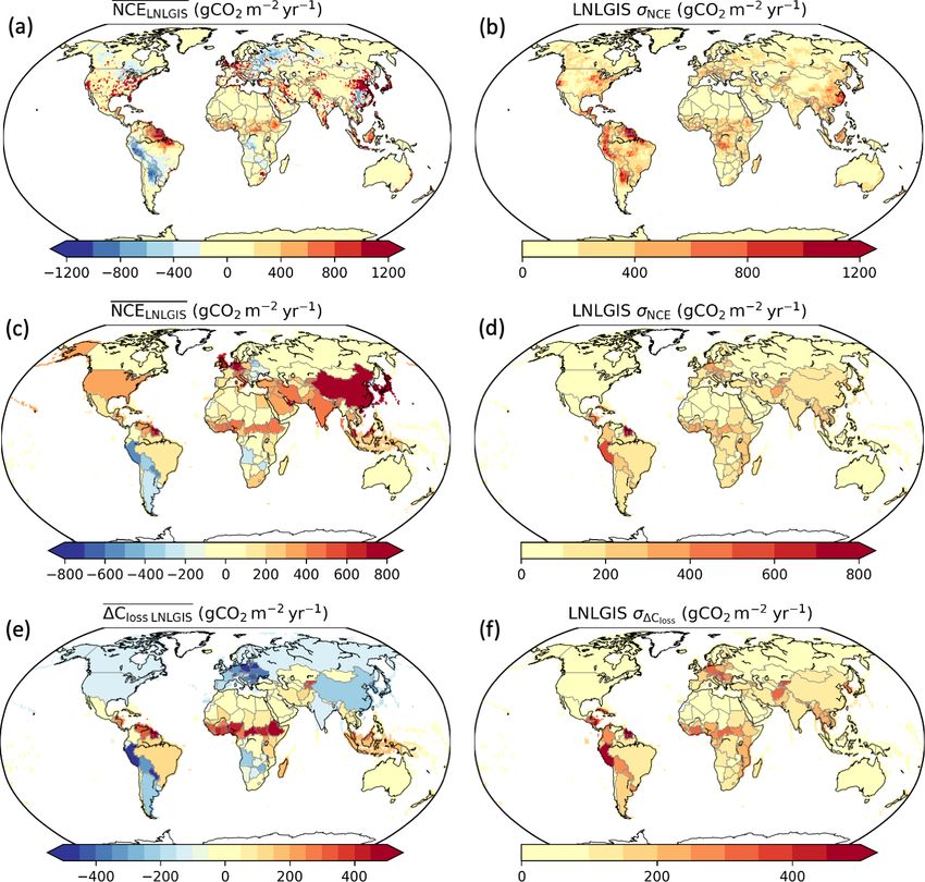
964                                                                                    B. Byrne et al.: Top-down CO2 budgets

                     21 Earth       Science Division, NASA Ames Research Center, Moffett Field, CA, USA
               22 Space        and Earth Observation Centre, Finnish Meteorological Institute, Sodankylä, Finland
          23 Division of Geological and Planetary Sciences, California Institute of Technology, Pasadena, CA, USA
               24 Laboratory of Numerical Modeling for Atmospheric Sciences & Geophysical Fluid Dynamics,

                           Institute of Atmospheric Physics, Chinese Academy of Sciences, Beijing, China
                        25 Department of Environmental Health and Engineering, Johns Hopkins University,

                                                           Baltimore, MD, USA
                            26 Institute of Environmental Physics, University of Bremen, Bremen, Germany
                27 Earth from Space Institute, Universities Space Research Association, Washington, D.C., USA
            28 Department of Atmospheric and Oceanic Science, University of Maryland, College Park, MD, USA
                                   29 Global Atmosphere Watch Team, Climate Research Department,

                      National Institute of Meteorological Sciences, Seogwipo-si, Jeju-do, Republic of Korea
               30 Research Institute for Global Change, Japan Agency for Marine-Earth Science and Technology

                                                     (JAMSTEC), Yokohama, Japan
                   31 Centre for Atmospheric Sciences, Indian Institute of Technology Delhi, New Delhi, India
                    32 National Institute of Water & Atmospheric Research Ltd (NIWA), Lauder, New Zealand
                          33 Royal Belgian Institute for Space Aeronomy (BIRA-IASB), Brussels, Belgium
                                     34 Japan Aerospace Exploration Agency (JAXA), Tsukuba, Japan
       35 Laboratoire d’Etudes du Rayonnement et de la Matière en Astrophysique et Atmosphères (LERMA-IPSL),

                     Sorbonne Université, CNRS, Observatoire de Paris, PSL Université, 75005 Paris, France
                       36 International Center for Climate and Global Change Research, College of Forestry,

                                     Wildlife and Environment, Auburn University, Auburn, AL, USA
       37 Schiller Institute for Integrated Science and Society, and Department of Earth and Environmental Sciences,

                                                 Boston College, Chestnut Hill, MA, USA
                                      38 Deutscher Wetterdienst (DWD), Hohenpeissenberg, Germany
                 39 Climate and Atmosphere Research Center (CARE-C), The Cyprus Institute, Nicosia, Cyprus

                             Correspondence: Brendan Byrne (brendan.k.byrne@jpl.nasa.gov)

                                      Received: 24 June 2022 – Discussion started: 12 July 2022
                          Revised: 8 December 2022 – Accepted: 17 January 2023 – Published: 7 March 2023

      Abstract. Accurate accounting of emissions and removals of CO2 is critical for the planning and verification of
      emission reduction targets in support of the Paris Agreement. Here, we present a pilot dataset of country-specific
      net carbon exchange (NCE; fossil plus terrestrial ecosystem fluxes) and terrestrial carbon stock changes aimed
      at informing countries’ carbon budgets. These estimates are based on “top-down” NCE outputs from the v10 Or-
      biting Carbon Observatory (OCO-2) modeling intercomparison project (MIP), wherein an ensemble of inverse
      modeling groups conducted standardized experiments assimilating OCO-2 column-averaged dry-air mole frac-
      tion (XCO2 ) retrievals (ACOS v10), in situ CO2 measurements or combinations of these data. The v10 OCO-2
      MIP NCE estimates are combined with “bottom-up” estimates of fossil fuel emissions and lateral carbon fluxes
      to estimate changes in terrestrial carbon stocks, which are impacted by anthropogenic and natural drivers. These
      flux and stock change estimates are reported annually (2015–2020) as both a global 1◦ × 1◦ gridded dataset
      and a country-level dataset and are available for download from the Committee on Earth Observation Satel-
      lites’ (CEOS) website: https://doi.org/10.48588/npf6-sw92 (Byrne et al., 2022). Across the v10 OCO-2 MIP
      experiments, we obtain increases in the ensemble median terrestrial carbon stocks of 3.29–4.58 Pg CO2 yr−1
      (0.90–1.25 Pg C yr−1 ). This is a result of broad increases in terrestrial carbon stocks across the northern extra-
      tropics, while the tropics generally have stock losses but with considerable regional variability and differences
      between v10 OCO-2 MIP experiments. We discuss the state of the science for tracking emissions and removals
      using top-down methods, including current limitations and future developments towards top-down monitoring
      and verification systems.

Earth Syst. Sci. Data, 15, 963–1004, 2023                                           https://doi.org/10.5194/essd-15-963-2023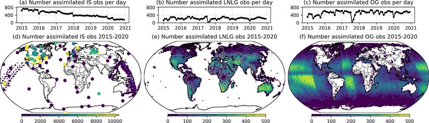
B. Byrne et al.: Top-down CO2 budgets                                                                                        965

Copyright statement. © 2023. California Institute of Technol-     CO2 mole fractions. These top-down methods have un-
ogy. Government sponsorship acknowledged.                         dergone rapid improvements in recent years, as recog-
                                                                  nized in the 2019 Refinement to the 2006 IPCC Guide-
                                                                  lines for National GHG Inventories (IPCC, 2019). And, al-
1   Introduction                                                  though these methods were not deemed to be a standard
                                                                  tool for verification of conventional inventories, a number
To reduce the risks and impacts of climate change, the Paris      of countries (UK, Switzerland, USA and New Zealand)
Agreement aims to limit the global average temperature in-        have adopted atmospheric inverse modeling as a verification
crease to well below 2 ◦ C above pre-industrial levels and to     system in national inventory reports. Initially, these coun-
pursue efforts to limit these increases to less than 1.5 ◦ C.     tries have focused on non-CO2 gasses (e.g., EPA, 2022),
To this end, each Party to the Paris Agreement agreed to          but top-down assessments of the CO2 budget are now un-
prepare and communicate successive nationally determined          der development in New Zealand (https://niwa.co.nz/climate/
contributions (NDCs) of greenhouse gas (GHG) emission re-         research-projects/carbon-watch-nz, last access: 6 Febru-
ductions. Collective progress toward this goal of the Paris       ary 2023). Furthermore, significant investments towards
Agreement is evaluated in global stocktakes (GSTs), which         building anthropogenic CO2 emissions monitoring and ver-
are conducted at 5-year intervals; the first GST is scheduled     ification support capacity are ongoing within the European
in 2023. The outcome of each GST is then used as input, or        Commission’s Copernicus Program (see Sect. 9.2.1).
as a “ratchet mechanism”, for new NDCs that are meant to             In top-down CO2 flux estimation, the net surface–
encourage greater ambition.                                       atmosphere CO2 fluxes are inferred from atmospheric CO2
   In support of the first GST, Parties to the Paris Agreement    observations using state-of-the-art atmospheric CO2 inver-
are compiling national GHG inventories (NGHGIs) of emis-          sion systems (e.g., Peiro et al., 2022). This approach pro-
sions and removals, which are submitted to the United Na-         vides spatially and temporally resolved estimates of surface–
tions Framework Convention of Climate Change (UNFCCC)             atmosphere fluxes for land and ocean regions from which
and inform their progress toward the emission-reduction tar-      country-level annual land–atmosphere CO2 fluxes can be
gets in their individual NDCs. For these inventories, emis-       estimated. The impact of fossil fuel (and usually fire CO2
sions and removals are generally estimated using “bottom-         emissions) on the observations is accounted for in the in-
up” approaches, wherein CO2 emission estimates are based          versions by prescribing maps of those emissions and assum-
on activity data and emission factors, while CO2 removals by      ing that they are perfectly known. Thus, fossil fuel and fire
sinks are based on inventories of carbon stock changes and        CO2 emissions are not diagnosed yet by these inversions
models, following the methods specified in the 2006 Inter-        but net surface–atmosphere CO2 fluxes from the terrestrial
governmental Panel on Climate Change (IPCC) Guidelines            biosphere and oceans are. Terrestrial carbon stock changes
for National GHG Inventories (IPCC, 2006). This approach          can then be calculated by combining net surface–atmosphere
allows for explicit characterization of CO2 emissions and re-     CO2 fluxes with estimates of fossil fuel emissions and hor-
movals into five categories: energy; industrial processes and     izontal (“lateral”) fluxes occurring within the terrestrial bio-
product use (IPPU); agriculture; land use, land-use change        sphere or between the land and ocean (Kondo et al., 2020).
and forestry (LULUCF); and waste. Bottom-up methods can           One example of a lateral flux is harvested agricultural prod-
provide precise and accurate country-level emission esti-         ucts, where carbon is sequestered from the atmosphere by
mates when the activity data and emission factors are well        photosynthesis in one region, but then this carbon is har-
quantified and understood (Petrescu et al., 2021), such as for    vested and exported to another region as agricultural prod-
the fossil fuel combustion category of the energy sector in       ucts. Similarly, carbon sequestered by photosynthesis in a
many countries. However, these estimates can have consid-         forest can be leached away by streams and rivers and then
erable uncertainty when the emission processes are challeng-      exported to the ocean. These lateral carbon fluxes are not di-
ing to quantify (such as for agriculture, LULUCF and waste)       rectly identifiable in atmospheric CO2 measurements, but ac-
or if the activity data are inaccurate or missing. For exam-      counting for their impact is required in order to convert net
ple, Grassi et al. (2022) and McGlynn et al. (2022) estimate      land fluxes into stock changes. These estimated terrestrial
the uncertainty on the net LULUCF CO2 flux to be roughly          carbon stock changes reflect the combined impact of direct
35 % for Annex I countries and 50 % for non-Annex I coun-         anthropogenic activities and changes to both managed and
tries. In addition, these estimates do not capture carbon emis-   unmanaged ecosystems in response to rising CO2 , climate
sions and removals from unmanaged systems, which are not          change and disturbance events (such as fires).
directly considered in the Paris Agreement, but impact the           The top-down budgets presented here extend several pre-
global carbon budget and growth rate of atmospheric CO2 .         vious studies that have developed approaches to compare in-
   As a complement to these accounting-based inventory ef-        version results to NGHGIs. Ciais et al. (2021) proposed a
forts, an independent “top-down” assessment of net surface–       protocol for reporting bottom-up and top-down fluxes so that
atmosphere CO2 fluxes may be obtained from ground-                they can be compared consistently. Petrescu et al. (2021)
based, airborne and space-based observations of atmospheric       compared top-down fluxes with inventory estimates for the

https://doi.org/10.5194/essd-15-963-2023                                          Earth Syst. Sci. Data, 15, 963–1004, 2023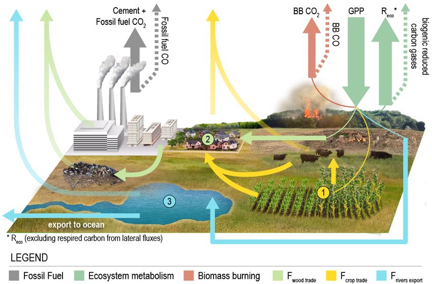
966                                                                                     B. Byrne et al.: Top-down CO2 budgets

European Union and UK, including for an ensemble of re-             carbon stocks. These products are provided annually over the
gional inversions over Europe (Monteil et al., 2020). Cheval-       6-year period 2015–2020 both on a 1◦ × 1◦ global grid and
lier (2021) noted that inversion results for terrestrial CO2        as country-level totals with error characterization.
fluxes should be restricted to managed lands and applied a             These products are intended to be used to help inform in-
managed land mask to the gridded fluxes of the Copernicus           ventory development and identify areas for future research in
Atmosphere Monitoring Service (CAMS) CO2 inversions for             both top-down and bottom-up approaches, including inform-
the comparison to UNFCCC values in 10 large countries or            ing strategies for operational top-down carbon cycle products
groups of countries. Deng et al. (2022) compared CO2 , CH4          that can be used for tracking combined changes in managed
and N2 O fluxes from inversion ensembles available from the         and unmanaged carbon stocks and that can help quantify the
Global Carbon Project. For CO2 , they used six CO2 flux es-         impact of emission reduction activities.
timates from inverse models that assimilated measurements
from the global air-sample network, filtered their results over     1.2   Overview of the carbon cycle
managed lands and corrected them for CO2 fluxes induced
by lateral processes to compare with carbon stock changes           The burning of fossil fuels and cement production release
reported to the UNFCCC by a set of 12 countries. We expand          geologic carbon to the atmosphere (40.0 ± 3.3 Pg CO2 yr−1
upon these previous studies by providing top-down CO2 bud-          or 10.9 ± 0.9 Pg C yr−1 over 2010–2019; Canadell et al.,
gets from the v10 Orbiting Carbon Observatory Model Inter-          2021). These emissions, along with land-use activities, im-
comparison Project (v10 OCO-2 MIP), wherein an ensemble             pact carbon cycling between atmospheric, oceanic and bio-
of inverse modeling groups conducted standardized exper-            spheric reservoirs that make up a near-closed system on an-
iments assimilating OCO-2 column-averaged dry-air mole              nual timescales. As a result, roughly half of the emitted CO2
fraction (XCO2 ) retrievals (retrieved with version 10 of the       from anthropogenic sources is absorbed by terrestrial ecosys-
Atmospheric CO2 Observations from Space (ACOS) full-                tems and oceans (Friedlingstein et al., 2022), reducing the
physics retrieval algorithm), in situ CO2 measurements or           rate of atmospheric CO2 increase (18.7±0.08 Pg CO2 yr−1 or
combinations of these data. This allows us to quantify the          5.1 ± 0.02 Pg C yr−1 over 2010–2019; Canadell et al., 2021).
sensitivity of top-down carbon budget estimates to the inver-       Here we briefly review the movement of carbon between the
sion modeling system and the atmospheric CO2 dataset used           reservoirs and how these processes are modulated by human
to constrain flux estimates.                                        activities.
   This paper is outlined as follows. The remainder of Sect. 1         Fluxes of carbon between the atmosphere and ocean are
describes the objectives of this work (Sect. 1.1) and pro-          driven by the difference in partial pressures of CO2 be-
vides background information on both the global carbon cy-          tween seawater and air, resulting in roughly balancing fluxes
cle (Sect. 1.2) and top-down atmospheric CO2 inversions             from the ocean-to-atmosphere and atmosphere-to-ocean of
(Sect. 1.3). Section 2 defines the carbon cycle fluxes of in-       ∼ 293 Pg CO2 yr−1 (∼ 80 Pg C yr−1 ) each way (Ciais et al.,
terest. Section 3 describes the flux datasets and their uncer-      2013), with a residual net atmosphere-to-ocean flux due to
tainties, including fossil fuel emissions, the v10 OCO-2 MIP,       increasing atmospheric CO2 (9.2 ± 2.2 Pg CO2 yr−1 or 2.5 ±
riverine fluxes, wood fluxes, crop fluxes and the net terrestrial   0.6 Pg C yr−1 over 2010–2019; Canadell et al., 2021). Re-
carbon stock loss. Section 4 provides an evaluation of the v10      gional variations in the solubility and saturation of CO2 in
OCO-2 MIP flux estimates. Section 5 presents two metrics            ocean waters drive net fluxes, with net fluxes to the atmo-
for interpreting the top-down constraints on the CO2 budget.        sphere in upwelling regions, such as the eastern boundary
Section 6 gives a description of the dataset, Sect. 7 shows         of basins and in equatorial zones (McKinley et al., 2017).
the characteristics of the dataset, Sect. 8 demonstrates how        Meanwhile, there are net removals by the ocean in western
these data can be compared with national inventories, and           boundary currents and at extratropical latitudes (McKinley
Sect. 9 discusses current limitations and future directions.        et al., 2017). Within the oceans, circulation patterns, mixing
Section 10 describes the data availability. Finally, Sect. 11       and biologic activity act to redistribute carbon.
gives the conclusions of this study.                                   On land, terrestrial ecosystems remove atmospheric car-
                                                                    bon through photosynthesis, referred to as gross primary pro-
1.1   Objectives
                                                                    duction (GPP) (Fig. 1). GPP draws roughly 440 Pg CO2 yr−1
                                                                    (120 Pg C yr−1 ) from the atmosphere (Anav et al., 2015).
This is a pilot project designed to start a dialogue between        Roughly half of this carbon is emitted back to the atmo-
the top-down research community, inventory compilers and            sphere by plants through autotrophic respiration, while the
the GHG assessment community to identify ways that top-             remaining carbon is used to generate plant biomass and is
down CO2 flux estimates can help inform country-level car-          referred to as net primary production (NPP). On an annual
bon budgets (see Worden et al., 2022, for a similar pilot           basis, the carbon sequestered through NPP is roughly bal-
methane dataset). To meet this objective, the primary goal of       anced by carbon loss through a number of processes. The
this work is to provide two products: (1) annual net surface–       largest of these processes is heterotrophic respiration, which
atmosphere CO2 fluxes and (2) annual changes in terrestrial         is the respiratory emission of CO2 (from the dead organic

Earth Syst. Sci. Data, 15, 963–1004, 2023                                            https://doi.org/10.5194/essd-15-963-2023
B. Byrne et al.: Top-down CO2 budgets                                                                                        967

matter and soil carbon pools) by heterotrophic organisms,          sions and removals are less well quantified. Regional-scale
and accounts for 82 %–95 % of NPP (Randerson et al., 2002).        carbon sequestration can differ substantially from the global
The combination of heterotrophic and autotrophic respiration       mean and can be impacted by the regional climate, distur-
is called ecosystem respiration (Reco ). The remaining pro-        bance events (Frank et al., 2015; Wang et al., 2021) and an-
cesses have smaller magnitudes but are still critical for deter-   thropogenic activities (Caspersen et al., 2000; Harris et al.,
mining the carbon balance of ecosystems. Biomass burning,          2012). The need to better quantify regional-scale emissions
the emission of carbon to the atmosphere through combus-           and removals of carbon has motivated much of the recent
tion, releases roughly 7.3 Pg CO2 yr−1 (2 Pg C yr−1 ) to the       expansion of in situ CO2 observing networks, the launch of
atmosphere on an annual basis but with considerable interan-       space-based CO2 observing systems and the development of
nual variability (van der Werf et al., 2017). Carbon can also      CO2 inversion systems.
be emitted from the terrestrial biosphere to the atmosphere
in the form of carbon monoxide (CO), methane (CH4 ) and            1.3   Background on atmospheric CO2 inversions
other biologic volatile organic compounds (BVOCs), which
are oxidized to CO2 in the atmosphere. Rivers move carbon          Atmospheric CO2 inversions estimate the underlying net
in the form of dissolved inorganic carbon (DIC), dissolved         surface–atmosphere CO2 fluxes from atmospheric CO2 ob-
organic carbon (DOC) and particulate organic carbon (POC).         servations, and this is what is meant by the top-down ap-
This carbon of terrestrial origin is partly transported to the     proach (Bolin and Keeling, 1963; Tans et al., 1990; Enting
open ocean, partly released to the atmosphere from inland          et al., 1995; Gurney et al., 2002; Peiro et al., 2022). In this
waters and estuaries, and partly buried in aquatic or marine       approach, an atmospheric chemical transport model (CTM)
sediments. Finally, anthropogenic activities such as harvest-      is employed to relate surface–atmosphere CO2 fluxes to ob-
ing of crop and wood products result in lateral transport of       served atmospheric CO2 mole fractions. As an inverse prob-
carbon such that the removal of atmospheric CO2 through            lem, the upwind CO2 fluxes are estimated from the down-
NPP and emission of atmospheric CO2 through respiration            wind observed CO2 mole fractions. The surface CO2 fluxes
(e.g., decomposition in a landfill) or combustion (e.g., burn-     are adjusted so that forward-simulated CO2 mole fractions
ing of biofuels) occur in different regions. See Fig. 1 for an     better match the CO2 measurements while considering the
illustration of these fluxes.                                      uncertainty statistics on the observations, transport and prior
   Globally, there is a long-term net uptake of atmo-              surface fluxes.
spheric CO2 by the land (approximately −6.6 Pg CO2 yr−1                The atmospheric CO2 inversion problem is generally ill-
or −1.8 Pg C yr−1 over 2010–2019; Canadell et al., 2021),          posed such that the solution is underdetermined by the ob-
which is the residual of an emission due to net land-              servational constraints. In this case, additional information
use change (5.9 ± 2.6 Pg CO2 yr−1 or 1.6 ± 0.7 Pg C yr−1           is required to produce a unique solution and prevent over-
over 2010–2019; Canadell et al., 2021) and removal by              fitting of the data (Lawson and Hanson, 1995; Tarantola,
other terrestrial ecosystems (12.6 ± 3.3 Pg CO2 yr−1 or 3.4 ±      2005). Typically, this is performed using Bayesian inference,
0.9 Pg C yr−1 over 2010–2019; Canadell et al., 2021). This         where prior mean fluxes and their uncertainties provide addi-
removal is partially driven by direct feedbacks between in-        tional information required to estimate fluxes (Rayner et al.,
creasing CO2 and the biosphere, such as CO2 fertilization of       2019). Prior mean fluxes of net ecosystem exchange are
photosynthesis and increased water use efficiency. Carbon–         usually obtained from terrestrial biosphere models (such as
climate feedbacks also lead to both increases and decreases        CASA, ORCHIDEE and CARDAMOM), while prior mean
in terrestrial carbon stocks: for example, warming at high lat-    air–sea fluxes are derived from surface water partial pressure
itudes leads to a more productive biosphere, but it also leads     of CO2 (pCO2 ) datasets or from ocean models (e.g., Peiro
to increased plant and soil respiration (Kaushik et al., 2020;     et al., 2022). The resulting posterior flux estimates combine
Walker et al., 2021; Canadell et al., 2021; Crisp et al., 2022).   the constraints on surface fluxes from atmospheric CO2 data
In addition, the release of nitrogen through anthropogenic         with the prior knowledge of the fluxes. If there is a high
energy and fertilizer use may drive increased carbon seques-       density of assimilated CO2 observations, then the posterior
tration by the terrestrial biosphere (Schulte-Uebbing et al.,      fluxes will be more strongly impacted by the assimilated
2022; Y. Liu et al., 2022; Lu et al., 2021). Regrowth of forests   data, whereas, in regions with sparse observational coverage,
in previously cleared areas, especially in the extratropics, is    the posterior fluxes will generally remain similar to the prior
also thought to be an important uptake term (Kondo et al.,         fluxes (assuming similar prior flux uncertainties across re-
2018; Cook-Patton et al., 2020). Currently, the relative im-       gions).
pact of each of these contributions to long-term terrestrial           Measurements of atmospheric CO2 best inform diffuse
carbon sequestration is poorly known and likely varies be-         biosphere–atmosphere fluxes on large spatial scales. This is
tween biomes and climates.                                         because CO2 has a long atmospheric lifetime such that the
   While the existence of a long-term global land sink is sup-     perturbation to atmospheric CO2 due to emissions and re-
ported through a number of lines of evidence (Ballantyne           movals from individual processes and locations gets mixed
et al., 2012; Keeling and Graven, 2021), regional-scale emis-      in the atmosphere (Gloor et al., 2001; Liu et al., 2015). For

https://doi.org/10.5194/essd-15-963-2023                                           Earth Syst. Sci. Data, 15, 963–1004, 2023
968                                                                                             B. Byrne et al.: Top-down CO2 budgets

Figure 1. CO2 is removed from the atmosphere through photosynthesis (GPP) and then emitted back to the atmosphere through a number
of processes. Three processes move carbon laterally on Earth’s surface such that emissions of CO2 occur in a different region than removals.
(1) Agriculture: harvested crops are transported to urban areas and to livestock, which are themselves exported to urban areas. CO2 is respired
to the atmosphere in livestock or urban areas. (2) Forestry: logged carbon is transported to urban and industrial areas, then emitted through
decomposition in a landfill or combustion as a biofuel. (3) Water cycle: carbon is leached from soils into water bodies, such as lakes. The
carbon is then either deposited, released to the atmosphere or transported to the ocean (Regnier et al., 2022). Arrows show carbon fluxes, and
colors indicate whether the flux is associated with (grey) fossil fuel emissions, (dark green) ecosystem metabolism, (red) biomass burning,
(light green) forestry, (yellow) agriculture or (blue) the water cycle. Semi-transparent arrows show fluxes that move between the surface and
atmosphere, while solid arrows show fluxes that move between land regions. Dashed arrows show surface–atmosphere fluxes of reduced
carbon species that are oxidized to CO2 in the atmosphere. For simplicity, a cement carbonation sink, volcano emissions and a weathering
sink are not included in this figure.

example, the measurements of CO2 at Mauna Loa, Hawaii,                    biases may be present. However, OCO-2 XCO2 retrievals over
provide a good estimate of the global-scale changes of CO2                oceans may contain more large-scale spatially coherent re-
surface fluxes. Inferring smaller-scale flux signals requires             trieval errors that can adversely impact flux estimates.
a high density of CO2 observations (to capture gradients                     Accurate atmospheric transport is critical for correctly
in atmospheric CO2 ) and accurate modeling of atmospheric                 relating surface–atmosphere fluxes to observations. Due to
transport (to relate the measurements with surface fluxes).               computational constraints, CTMs are typically run offline
The accuracy of flux estimates depends on a number of                     with coarsened meteorological fields relative to the parent
factors, particularly the accuracy and precision of the data,             numerical weather prediction model, which has been shown
transport model and prior constraints. Stringent requirements             to introduce systematic transport errors in some configura-
on the accuracy of space-based column-averaged dry-air                    tions (Yu et al., 2018; Stanevich et al., 2020). In addition,
mole fraction (XCO2 ) retrievals are required to infer surface            these offline CTMs have been shown to have large-scale sys-
fluxes (Chevallier et al., 2005a; Miller et al., 2007). Biases            tematic differences in transport associated with the imple-
in XCO2 retrievals from the Orbiting Carbon Observatory                   mentation of transport algorithms (Schuh et al., 2019, 2022).
(OCO-2) related to spectroscopic errors, solar zenith angle,              These errors appear to be of the same order as the retrieval
surface properties, and atmospheric scattering by clouds and              biases, although the patterns in time and space are differ-
aerosols have been identified (Wunch et al., 2017b). How-                 ent. Systematic errors related to model transport (and er-
ever, intensive research has reduced retrieval errors over time           rors in prior information) can partially be accounted for by
(O’Dell et al., 2018; Kiel et al., 2019). As will be shown                performing multiple inversions that differ in CTM and prior
in Sect. 4.1, biases in OCO-2 XCO2 retrievals over land are               constraints employed. This motivates inversion model inter-
thought to be relatively small, although regionally structured            comparison projects (MIPs), such as the OCO-2 MIP project

Earth Syst. Sci. Data, 15, 963–1004, 2023                                                    https://doi.org/10.5194/essd-15-963-2023
B. Byrne et al.: Top-down CO2 budgets                                                                                            969

(see Sect. 3.2; Crowell et al., 2019; Peiro et al., 2022). From            – Net terrestrial carbon stock gain (1Cgain ). Positive
these ensembles of inversions, estimates of both systematic                  values indicate a gain (increase) of terrestrial carbon
errors (accuracy) and random errors (precision) can be ob-                   stocks, and this is the negative of 1Closs :
tained from the model spread.
                                                                              1Cgain = −1Closs .                                  (3)
2    Definitions

In this work, we focus on the carbon budget of Earth’s land            Country and regional aggregation
area, including aquatic systems such as rivers and lakes. In
particular, we consider fluxes of carbon between the land and          To aggregate gridded 1◦ × 1◦ flux estimates to country to-
the atmosphere and lateral carbon transport processes on land          tals we use a country mask (Center for International Earth
and between the land and ocean (Fig. 1). We define the fol-            Science Information Network – CIESIN – Columbia Uni-
lowing annual net carbon fluxes (see Fig. 2 for a schematic            versity, 2018). We also provide NCE and 1Closs estimates
representation of these fluxes):                                       for several country groupings. A number of regional inter-
                                                                       governmental organizations are included: the Association of
    – Fossil fuel and cement emissions (FF). The burning of            Southeast Asian Nations (ASEAN), the African Union (AU)
      fossil fuels and release of carbon due to cement produc-         and each of its sub-regions (North, South, West, East and
      tion, representing a flux of carbon from the land surface        Central), the Community of Latin American and Caribbean
      (geologic reservoir) to the atmosphere.                          States plus Brazil (CELAC+Brazil), the Economic Coopera-
                                                                       tion Organization (ECO), the European Union (EU or EU27),
    – Net biosphere exchange (NBE). Net flux of carbon                 and the South Asian Association for Regional Cooperation
      from the terrestrial biosphere to the atmosphere due to          (SAARC). We also include some geographic regions, specif-
      biomass burning (BB) and Reco minus gross primary                ically North America, the Middle East and Europe. Coun-
      production (GPP) (i.e., NBE = BB+Reco −GPP). It in-              tries included in these groupings are listed in the Supplement
      cludes both anthropogenic processes (e.g., deforesta-            (Text S1).
      tion, reforestation, farming) and natural processes (e.g.,
      climate-variability-induced carbon fluxes, disturbances,
                                                                       3     Flux datasets
      recovery from disturbances).

    – Terrestrial net carbon exchange (NCE). Net flux of car-          Here, we describe the methodologies and datasets for esti-
      bon from the surface to the atmosphere. For land, NCE            mating FF (Sect. 3.1), NCE (Sect. 3.2) and lateral carbon
      can be defined as                                                fluxes (Sect. 3.3), as well as how these data are used to esti-
                                                                       mate 1Closs (Sect. 3.4).
      NCE = NBE + FF.                                           (1)
                                                                       3.1    Fossil fuel and cement emissions
    – Lateral crop flux (Fcrop trade ). The lateral flux of carbon     Gridded 1◦ × 1◦ fossil CO2 emissions, including those from
      in (positive) or out (negative) of a region due to agricul-      cement production, are calculated as follows. Monthly grid-
      ture.                                                            ded emissions up to 2019 are taken from the 2020 version
                                                                       of the Open-source Data Inventory for Anthropogenic CO2
    – Lateral wood flux (Fwood trade ). The lateral flux of car-
                                                                       (ODIAC2020, 2000–2019) emission data product (Oda and
      bon in (positive) or out (negative) of a region due to
                                                                       Maksyutov, 2011; Oda et al., 2018). The 2020 emissions
      wood product harvesting and usage.
                                                                       were not part of ODIAC but were projected using the Carbon
    – Lateral river flux (Frivers export ). The lateral flux of car-   Monitor (CM) emission data product (https://carbonmonitor.
      bon in (positive) or out (negative) of a region trans-           org/, last access: 19 May 2021). For each month in 2020
      ported by the water cycle.                                       and later, the ratio between that month’s emissions and the
                                                                       emissions from the same month in 2019 was calculated from
    – Net terrestrial carbon stock loss (1Closs ). Positive val-       the CM emission data. Since CM provides daily emissions
      ues indicate a loss (decrease) of terrestrial carbon stocks      per sector for a handful of major emitting countries and the
      (organic matter stored on land), including above- and            globe, CM emissions are summed over sectors and days in
      below-ground biomass in ecosystems and biomass con-              each month to create monthly total emissions per named
      tained in anthropogenic products (lumber, cattle, etc.).         country and the rest of the world (RoW). The ratio of each
      This is calculated as                                            (post-2019) month’s emission to the same month in 2019 is
                                                                       then calculated per named country and RoW, then distributed
      1Closs = NBE − Fcrop trade − Fwood trade                         over a 1◦ × 1◦ grid assuming homogeneity of the ratio over
              − Frivers export .                                (2)    each named country and RoW. The 2019 ODIAC emissions

https://doi.org/10.5194/essd-15-963-2023                                                Earth Syst. Sci. Data, 15, 963–1004, 2023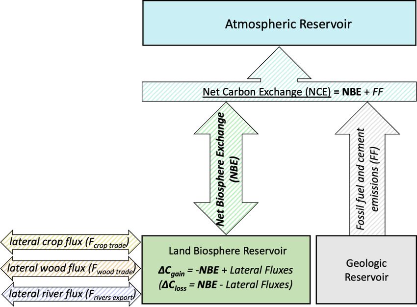
970                                                                                           B. Byrne et al.: Top-down CO2 budgets

Figure 2. Carbon fluxes for a given land region, such as a country. Boxes with solid backgrounds show reservoirs of carbon. Arrows
with hatched shading show fluxes between reservoirs. NCE is underlined to emphasize that this quantity is estimated from the atmo-
spheric CO2 measurements using top-down methods. Italicized quantities are obtained from bottom-up datasets (FF, Fcrop trade , Fwood trade ,
Frivers export ). Bold quantities are derived in this study from the top-down and bottom-up datasets (NBE, 1Cgain , 1Closs ).

for that month are then multiplied by the ratio to generate             elers that produces ensembles of CO2 surface–atmosphere
1◦ × 1◦ monthly emissions after 2019. While this method                 flux estimates by assimilating space-based OCO-2 retrievals
loses the information of day-to-day variability provided by             of XCO2 and in situ CO2 measurements. The v10 OCO-2
CM, this is a conscious choice to be consistent over the entire         MIP is updated from the v9 OCO-2 MIP described in Peiro
inversion period. Finally, we impose day-of-week and hour-              et al. (2022). Updates to the v10 OCO-2 MIP are presented
of-day variations on these fluxes following the Temporal Im-            here with additional details available at https://gml.noaa.gov/
provements for Modeling Emissions by Scaling (TIMES)                    ccgg/OCO2_v10mip/ (last access: 6 February 2023).
diurnal and day-of-week scaling (Nassar et al., 2013). The                 The v10 OCO-2 MIP consists of a number of inversion
1◦ × 1◦ uncertainty map is based on the combination of the              systems that perform a set of experiments following a stan-
global level FF uncertainty (1σ of 4.2 %, Andres et al., 2014)          dard protocol. Here, we include fluxes from 11 of the 14
and the grid level emission differences due to the different            MIP models (Table 1; CMS-Flux and JHU were excluded
disaggregation methods (Oda et al., 2015). Note that these              due to time constraints, and LoFI was excluded because it
FF uncertainties are not considered in the inversions used for          employs a non-traditional inversion approach that does not
this product development.                                               follow the MIP protocol). There are five v10 OCO-2 MIP ex-
   Country-level fossil fuel emission estimates are obtained            periments that each ensemble member performs, which dif-
by aggregating the 1◦ × 1◦ estimates using the country mask.            fer by the data that are assimilated (CO2 datasets described
Uncertainties on country-level estimates are calculated using           in Sect. 3.2.1):
the fractional uncertainties of Andres et al. (2014).

3.2   Net carbon exchange (NCE) and net biosphere
      exchange (NBE)
We employ results from the v10 OCO-2 MIP, which is an in-
ternational collaboration of atmospheric CO2 inversion mod-

Earth Syst. Sci. Data, 15, 963–1004, 2023                                                  https://doi.org/10.5194/essd-15-963-2023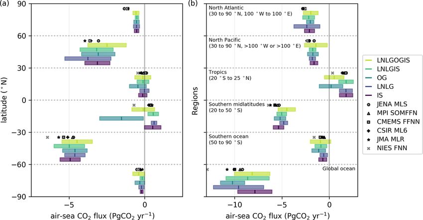
Table 1. Inversion specifications for each v10 OCO-2 MIP ensemble member. Note that since the creation of this table, the Global Carbon Assimilation System (GCAS; Jiang et al.,
                                            2021) has also contributed an ensemble member.

                                             Simulation name                         Transport                     Driving                        Meteorology                   Prior NEE                      Prior air–sea       Prior fire    Inverse
                                             (reference)                             model                         meteorology                    resolution (◦ )                                                                                method
                                             AMES                                    GEOS-Chem                     MERRA-2                        4◦ × 5◦                       CASA-GFED4.1s                  CT2019OI            GFEDv4.1s     4D-Var
                                             (Philip et al., 2019, 2022)
                                             Baker                                   PCTM                          MERRA-2                        1◦ × 1.25◦ prior,             CASA-GFED3                     Landschützer v4.4   GFEDv4        4D-Var
                                             (D. F. Baker et al., 2006; Baker                                                                     4◦ × 5◦ opt
                                             et al., 2010)
                                                                                                                                                                                                                                                                      B. Byrne et al.: Top-down CO2 budgets

                                             CAMS                                    LMDz                          ERA5                           1.9◦ × 3.75◦                  ORCHIDEE (climato-             CMEMS               GFED4.1s      Variational

https://doi.org/10.5194/essd-15-963-2023
                                             (Chevallier et al., 2005b)                                                                                                         logical)
                                             CMS-Fluxa                               GEOS-Chem                     MERRA-2                        4◦ × 5◦                       CARDAMOM                       MOM-6               CARDAMOM      4D-Var
                                             (J. Liu et al., 2021)
                                             COLA                                    GEOS-Chem                     MERRA-2                        4◦ × 5◦                       VEGAS                          Rödenbeck 2021      VEGAS         EnKF
                                             (Z. Liu et al., 2022)
                                             CSU                                     GEOS-Chem                     MERRA-2                        4◦ × 5◦                       SiB-4 w/MERRA-2                Landschützer v18    GFED4.1s      synthesis
                                             CT                                      TM5                           ERA5                           2◦ × 3◦ /                     CT2019 CASA                    CT2019OI            CT2019 CASA   EnKF
                                             (Jacobson et al., 2020)                                                                              1◦ × 1◦                       GFED4.1s                                           GFED4.1s
                                             JHUa                                    GEOS-Chem                     MERRA-2                        4◦ × 5◦                       CASA-GFED 4.1s                 Takahashi           GFED4.1s      geostatistical/4D-
                                             (Miller et al., 2020)                                                                                                                                                                               Var
                                             (Chen et al., 2021b, a)
                                             LoFIb                                   GEOS GCM                      GEOS CGM                       0.5◦ × 0.625◦                 CASA-GFED3                     LoFI Takahasi       QFED          n/a
                                             (Weir et al., 2021a, b)
                                             NIES                                    NIES-TM/FLEXPART              ERA5/JRA-55                    3.75◦ × 3.75◦ /               Zeng 2020                      Landschützer 2020   GFAS          4D-Var
                                             (Maksyutov et al., 2021)                                                                             0.1◦ × 0.1◦
                                             OU                                      TM5                           ERA-Interim                    4◦ × 6◦                       CASA-GFED3                     Takahashi           GFEDv3        4D-Var
                                             TM5-4DVar                               TM5                           ERA-Interim                    2◦ × 3◦                       SiB-CASA                       CT2019              GFEDv4        4D-Var
                                                                                                                                                                                                               Opt Clim
                                             UT                                      GEOS-Chem                     GEOS-FP                        4◦ × 5◦                       BEPS                           Takahashi           GFEDv4        4D-Var
                                             (Deng et al., 2014, 2016)
                                             WOMBAT                                  GEOS-Chem                     MERRA-2                        2◦ × 2.5◦                     SiB-4 w/MERRA-2                Landschutzer 2020   GFED4.1s      Synthesis
                                             (Zammit-Mangion et al., 2022)                                                                                                                                                                       with MCMC

                                            a Due to time constraints, this ensemble member is not included in this product. b This is not a traditional inversion and is not included in this product. n/a: not applicable.

Earth Syst. Sci. Data, 15, 963–1004, 2023
                                                                                                                                                                                                                                                                          971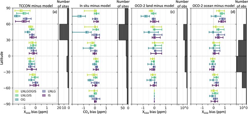
972 B. Byrne et al.: Top-down CO2 budgets
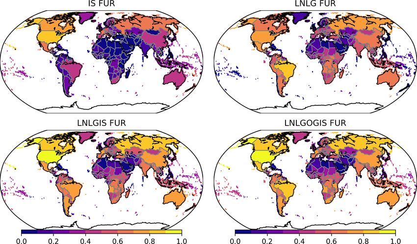
– IS assimilates in situ CO2 mole fraction measurements cells. Thus, first aggregating regions for each ensemble mem-
from an international observational network. ber accurately propagates the aggregate differences between
regions across the ensemble members.
– LNLG assimilates ACOS v10 land nadir and land glint The NBE estimate is calculated by subtracting the ODIAC
total column dry-air mole fractions (XCO2 ) from OCO- fossil fuel emissions from NCE. The variance in NBE is then
2. taken to be the sum of the variances of NCE and FF:
2 2 2
– LNLGIS assimilates both in situ and ACOS v10 OCO-2 σNBE = σNCE + σFF . (5)
land nadir and glint XCO2 retrievals together.
– OG assimilates ACOS v10 OCO-2 ocean glint XCO2 re-
trievals 3.2.1 Atmospheric CO2 data included in v10 OCO-2
MIP
– LNLGOGIS assimilates all the above datasets together.
In situ CO2 measurements (Fig. 3a and d) are drawn from five
data collections made available in ObsPack format (Masarie
For each experiment, each inversion group imposes a com-
et al., 2014). Those source ObsPacks and their references
mon fossil fuel emission dataset identical to the one de-
are listed in Table 2. These data include measurements from
scribed in Sect. 3.1. All other prior flux estimates were cho-
55 international laboratories at 460 sites around the world.
sen independently by each modeling group and are listed
The majority of data are from the openly available GLOB-
in Table 1. The inversions assimilate the standardized v10
ALVIEW+ program but with some additional provisional
OCO-2 and in situ data from 6 September 2014 through
data for 2020–2021 and data from other programs not partic-
31 March 2021 (see Sect 3.2.1), with the length of spin-
ipating in the GLOBALVIEW+ project. CO2 measurements
up period and in situ data assimilated during that period
are broadly divided into two categories: those measurements
being left up to the discretion of each group in the MIP.
we identify as suitable for assimilation and other measure-
Each modeling group submitted net air–sea fluxes and NBE
ments not suitable for assimilation.
across 2015–2020, interpolated from the native resolution to
In CO2 inverse analyses, uncertainties ascribed to in situ
a 1◦ × 1◦ spatial grid at monthly resolution, which are pub-
measurements are a combination of the uncertainty in the
licly available for download from https://gml.noaa.gov/ccgg/
measurement and a representativeness error from the inabil-
OCO2_v10mip/ (last access: 6 February 2023).
ity of the forward model to accurately simulate the measure-
The performance of each atmospheric CO2 inversion was
ment (due to aspects like a coarse model grid). To character-
evaluated through comparisons of the posterior CO2 mole-
ize the representativeness error, we used an empirical scheme
fraction field (i.e., CO2 fields simulated forward with the pos-
based on simulations from the v7 OCO-2 MIP (Crowell et al.,
terior fluxes) against independent in situ CO2 measurements
2019). In situ CO2 measurements are simulated in a for-
and OCO-2 XCO2 retrievals that were withheld from the as-
ward simulation, and then the model–data mismatch statistics
similation for validation, as well as XCO2 retrievals from the
are calculated to characterize the representativeness errors at
Total Column Carbon Observing Network (TCCON; Wunch
each measurement location and for each season. Although
et al., 2011). The evaluation of the experiments is presented
this was the standard method for characterizing uncertain-
in Sect. 4, with additional analysis available from the v10
ties for modeled in situ measurements, each v10 OCO-2 MIP
OCO-2 MIP website.
group was free to choose how to set the uncertainties in their
For this study, the best estimate of NCE is taken to
specific setups.
be the ensemble median for each experiment (denoted
Of the in situ measurements designated as being appro-
NCEexperiment ). The uncertainty in NCE is calculated as an
priate for assimilation, about 5 % were withheld for cross-
estimate (denoted σNCE ) of the distribution’s standard devi-
validation purposes. These data were chosen to be as inde-
ation using the interquartile range (IQR) of the v10 OCO-
pendent as possible from the measurements that were as-
2 MIP ensemble. It is a robust estimate that requires only
similated. For quasi-continuous measurements, such as those
the middle 50 % of the ensemble to be normally distributed
taken every 15 min at NOAA tall towers, measurements were
(Hoaglin et al., 1985). Hence from the normal tables, to two
withheld for entire days: we chose 5 % of the days in the
decimal places,
dataset, and we withheld every assimilable measurement on
IQR(NCE) that day. This is also how CO2 measurements on National In-
σNCE = . (4) stitute for Environmental Studies (NIES) ships were treated.
1.35
Entire aircraft profiles in the NOAA light-aircraft profiling
For country-level fluxes, the NCE estimates are first aggre- network are assumed to consist of vertically correlated mea-
gated to country totals for each ensemble member before surements, so entire profiles were withheld: we chose 5 % of
calculating the median and standard deviation. This is done aircraft profiles to withhold. Most flask sites have measure-
because there are spatial covariances between 1◦ × 1◦ grid ment sampling protocols intended to ensure independence;
Earth Syst. Sci. Data, 15, 963–1004, 2023 https://doi.org/10.5194/essd-15-963-2023B. Byrne et al.: Top-down CO2 budgets 973
Figure 3. Assimilated observations for IS, LNLG and OG v10 MIP experiments. Number of monthly (a) in situ CO2 measurements and
(b) ACOS v10 OCO-2 land nadir and land glint XCO2 retrievals binned into 10 s averages and (c) ACOS v10 OCO-2 ocean glint XCO2
retrievals binned into 10 s averages. Spatial distribution of (d) in situ (e) ACOS v10 OCO-2 land XCO2 retrievals and (f) ACOS v10 OCO-2
ocean XCO2 retrievals over 2015–2020. Shipboard and aircraft in situ CO2 measurements are aggregated to a 2◦ × 2◦ spatial grid, surface
site measurements are shown as scattered points and ACOS v10 OCO-2 XCO2 retrievals are shown aggregated to a 2◦ × 2◦ spatial grid.
Table 2. In situ CO2 measurement collections used in the v10 OCO-2 MIP, with the total number of measurements between 6 Septem-
ber 2014 and 1 January 2021 and the numbers of measurements assimilated and withheld for cross-validation in the same period. More
than 95 % of the in situ measurements come from the GLOBALVIEW+ and CO2 NRT ObsPacks, both of which are publicly available at
https://gml.noaa.gov/ccgg/obspack/data.php.
ObsPack name Total no. Assimilated Withheld Reference
measurements
obspack_CO2 _1_GLOBALVIEWplus_v6.1_2021-03-01 9 611 095 766 179 38 483 Schuldt et al. (2021b)
obspack_CO2 _1_NRT_v6.1.1_2021-05-17 755 477 62 011 2996 Schuldt et al. (2021a)
obspack_CO2 _1_NIES_Shipboard_v3.0_2020-11-10 418 496 216 963 12 766 Tohjima et al. (2005);
Nara et al. (2017)
obspack_CO2 _1_AirCore_v4.0_2020-12-28 55 620 Baier et al. (2021)
obspack_multi-species_1_manaus_profiles_v1.0_2021-05-20 3194 Miller et al. (2021)
Total 10 843 882 1 045 153 54 245
they are often taken at weekly or biweekly intervals dur- ocean scenes are assumed when calculating the uncertainty
ing meteorological conditions meant to allow regional back- on the 10 s averages (see Sect. 3.2.1 of Baker et al., 2022);
ground air masses to be sampled. Thus, we chose to withhold transport model errors are also considered (based on Schuh
5 % of assimilable flask measurements. We also verified that et al., 2019). Only 10 s spans with 10 or more good quality
datasets at the same site were withheld on the same days; air- retrievals were used (sparser data being thought to be more
craft profiles over tower sites were, for instance, withheld on prone to cloud-related biases). In the same vein as was done
the same days that tower data were withheld. for the in situ data, XCO2 data from 5 % of the orbits (entire
OCO-2 land (Fig. 3b and e) and ocean (Fig. 3c and f) XCO2 orbits were withheld), chosen at random, were withheld for
retrievals are performed using version 10 of NASA’s ACOS evaluation purposes.
full-physics retrieval algorithm (O’Dell et al., 2018). A com-
mon set of OCO-2 retrieval “super-obs” data were derived 3.3 Lateral carbon fluxes
from these retrievals and were assimilated by each model-
ing group. These super-obs are obtained by aggregating re- Lateral carbon flux datasets (Table 3) include country-
trievals into 10 s averages (which better match the coarse level Frivers export (Sect. 3.3.1), country-level Fcrop trade and
transport models’ grid cells used in the inversions) follow- country-level Fwood trade (Sect. 3.3.2). Gridded lateral fluxes
ing the same procedure as the v9 OCO-2 MIP (Peiro et al., are estimated using a somewhat different approach and are
2022). Specifically, individual scenes within the 10 s span described in Sect. 3.3.3.
are weighted according to the inverse of the square of the
XCO2 uncertainty (standard deviations) produced by the re-
trieval, and correlations of +0.3 for land scenes and +0.6 for
https://doi.org/10.5194/essd-15-963-2023 Earth Syst. Sci. Data, 15, 963–1004, 2023974 B. Byrne et al.: Top-down CO2 budgets
Table 3. Data sources for lateral flux estimates.
Resolution Flux Model/data source Section
National Frivers export Dynamic Land Ecosystem Model (DLEM) and Global NEWS with COSCATs data Sect. 3.3.1
National Fwood trade UN FAO Sect. 3.3.2
National Fcrop trade UN FAO Sect. 3.3.2
1◦ × 1◦ Frivers export Global NEWS with COSCATs data Sect. 3.3.3
1◦ × 1◦ Fwood trade UN FAO with downscaling Sect. 3.3.3
1◦ × 1◦ Fcrop trade UN FAO with downscaling Sect. 3.3.3
3.3.1 Country-level Frivers export tions (modified from COSCATs) (Meybeck et al., 2006). To
estimate country totals, we map the basin carbon loss across
Rivers transport carbon laterally across land regions (e.g., to land by assuming that the net carbon flux occurs uniformly
a lake) and from the land to the ocean. This lateral transport across each basin. We then use the country mask to estimate
must be accounted for to quantify the total change in terres- the country totals for each region.
trial carbon in a given region. However, there is considerable Deng et al. (2022) estimate the lateral carbon export by
uncertainty in lateral carbon flux by rivers. To account for rivers to the coast minus the imports from rivers entering
this, we use two independent estimates of country-level to- in each country (for relevant cases), including DOC, POC
tals: one from the Dynamic Land Ecosystem Model (DLEM; and DIC of atmospheric origin. Estimates of DOC, POC and
Tian et al., 2010, 2015a) and the other based on Deng et al. DIC are obtained from the Global NEWS model (Mayorga
(2022), who use the Global NEWS model (Mayorga et al., et al., 2010), with a correction based on Resplandy et al.
2010) and observations across COastal Segmentation and re- (2018) so that the global total exported to the coastal ocean
lated CATchments (COSCATs; Meybeck et al., 2006) that is 2.86 Pg CO2 yr−1 (0.78 Pg C yr−1 ). Deng et al. (2022) per-
include dissolved inorganic carbon (DIC) of atmospheric ori- form a correction to the Global NEWS estimates to remove
gin, dissolved organic carbon (DOC) and particulate organic the contribution of lithogenic carbon, using the methodology
carbon (POC). These datasets cover 2015–2019. For 2020, of Ciais et al. (2021).
we impose the 2015–2019 mean. For the analysis that follows, we estimate country-level to-
The DLEM is a process-based terrestrial ecosystem model tals of riverine lateral carbon fluxes by combining the esti-
that couples biophysical, soil biogeochemical, plant phys- mates of DLEM with those of Deng et al. (2022). We take
iological and riverine processes with vegetation and land- the mean of the two estimates to be the best estimate and take
use dynamics to simulate and predict the vertical fluxes, lat- the magnitude of the difference between the estimates to be
eral fluxes, and storage of water, carbon, GHGs, and nutri- the 1σ uncertainty. Figure S1 shows the 2015–2019 mean an-
ent dynamics in terrestrial ecosystems and their interfaces nual net riverine lateral carbon fluxes. Fluxes are uniformly
with the atmosphere and land–ocean continuum (Tian et al., negative, implying a net flux of carbon from the land to the
2010, 2015a). There are three major processes involved in ocean and reduction in stored carbon for all countries. Fluxes
simulating the export of water, carbon and nutrients from are most negative in tropical rain forest and tropical monsoon
land surface to the coastal ocean: (1) the generation of runoff climates, and they are smallest in more arid regions.
and leachates; (2) the leaching of water, carbon, and nutri-
ents from land to river networks in the form of overland flow
3.3.2 Country-level Fwood trade and Fcrop trade
and base flow; and (3) transport of riverine materials along
river channels from upstream areas to coastal regions. The Wood and crop products are traded between nations. We esti-
key processes and parameterization in the DLEM have been mate the annual lateral fluxes of carbon due to this trade fol-
described in previous publications regarding the water dis- lowing the approaches of Deng et al. (2022) and Ciais et al.
charge (Liu et al., 2013; Tao et al., 2014), riverine carbon (2021). This approach utilizes crop and wood trade data com-
fluxes (Ren et al., 2015, 2016; Tian et al., 2015b; Yao et al., piled by the Food and Agriculture Organization of the United
2021) and riverine nitrogen fluxes (Yang et al., 2015; Tian Nations (FAO; http://www.fao.org/faostat/en/#data, last ac-
et al., 2020) from the terrestrial ecosystem to coastal oceans. cess: 6 February 2023). The crop flux was estimated from
The newly improved DLEM aquatic module better addresses the annual trade balance of 171 crop commodities calculated
processes within global small streams, which were recog- for each country. For wood products, we use the bookkeeping
nized as hotspots of GHG emissions (Yao et al., 2020, 2021). model of Mason Earles et al. (2012) to calculate the fraction
DLEM produces estimates of the land loadings of carbon of imported carbon in wood products that is oxidized in each
species (DIC, DOC and POC), CO2 degassing and carbon of 270 countries during subsequent years. The 1σ uncertain-
burial during transporting, and the exports of carbon (DIC, ties in country-level fluxes are assumed to be 30 % of the
DOC and POC) to the ocean for 105 basin-level segmenta- mean value. This dataset covers 2015–2019. For 2020, we
Earth Syst. Sci. Data, 15, 963–1004, 2023 https://doi.org/10.5194/essd-15-963-2023B. Byrne et al.: Top-down CO2 budgets 975
assume fluxes equal to the 2015–2019 mean. The net crop 2. XCO2 retrievals from the TCCON. These data are ac-
and wood lateral fluxes and their uncertainties are shown in quired from a network of ground-based Fourier trans-
Fig. S2. form spectrometers measuring direct solar spectra from
which XCO2 is retrieved (Wunch et al., 2011). For this
3.3.3 1◦ × 1◦ lateral flux estimates analysis, we include 30 TCCON sites listed in Table A1.
These data are filtered and aggregated following the
Lateral fluxes at a higher resolution (1◦ × 1◦ ) follow method outlined in Appendix C of Crowell et al. (2019).
similar principles to national values but were estimated
separately with different implementation choices. High- 3. Withheld OCO-2 land glint and land nadir XCO2 re-
resolution proxy data (satellite-derived NPP, population or trievals. These data could have been assimilated, but
livestock maps, etc.) enabled sub-national disaggregation. they are intentionally withheld for evaluation purposes
This was done using national totals based on FAO statis- (Sect. 3.2.1).
tics for Fwood trade and Fcrop trade . For Frivers export these es- 4. Withheld OCO-2 ocean glint XCO2 retrievals. These
timates were generated from Global NEWS and COSCATs data could have been assimilated, but they are intention-
data (DLEM was only used for national totals). For each ally withheld for evaluation purposes (Sect. 3.2.1).
1◦ × 1◦ grid cell, we assume the standard deviation of the
mean flux to be 30 % for Fwood trade and Fcrop trade and 60 % We first perform a simple check on the inversion results by
for Frivers export . These uncertainty estimates are based on ex- comparing the atmospheric CO2 growth rate estimated from
pert opinion, as a rigorous error budget has not yet been de- the v10 OCO-2 MIP experiments to that derived directly
veloped for the 1◦ × 1◦ lateral flux estimates. from NOAA CO2 measurements (Fig. 4). The growth rate is
estimated from CO2 measurements and model co-samples at
3.4 Estimate of carbon stock loss (∆Closs ) “marine boundary layer” sites, which predominantly observe
well-mixed marine boundary layer air representative of a
Finally, we calculate 1Closs using Eq. (2) with the datasets large volume of the atmosphere. A smooth curve is then fit to
described above. Assuming that the components contribut- these data to estimate the global growth rate (Thoning et al.,
ing to 1Closs are independent, we calculate the uncertainty 1989). This is the same method employed by NOAA to report
on 1Closs by combining the uncertainties (1 standard devia- the CO2 growth rate (http://www.gml.noaa.gov/ccgg/trends/,
tions) from the component fluxes in quadrature: last access: 6 February 2023). We estimate the uncertainty in
the measurement-based growth rate from the difference be-
2 2
σ1C loss
= σNBE + σF2crop trade
+ σF2wood trade
+ σF2rivers export
. (6) tween the growth rate estimated here and that reported on the
NOAA website. Differences between these estimates are pri-
4 Evaluation of v10 OCO-2 MIP experiments marily driven by differences in measurement sampling used
for the website relative to that used here (as we are limited
The performance of top-down CO2 flux estimates can be im- to withheld co-samples here). We calculate the uncertainty
pacted by a number of factors, including biases in the as- as the standard error of the mean for the differences between
similated data, model transport, prior constraints and inver- the growth rates estimated here and by NOAA across 2015–
sion architectures. Therefore, evaluating the performance of 2019. This gives an uncertainty on the 5-year growth rate of
v10 OCO-2 MIP fluxes against independent observational ±0.053 ppm yr−1 . Note that NOAA reports the growth rate
datasets is critical for assuring high-quality flux estimates. using the X2019 scale, whereas our estimates here are from
Here, we evaluate the v10 OCO-2 MIP experiments in two the X2007 scale, which may contribute to the differences. We
ways. First, we compare the posterior CO2 fields against in- find that the IS, LNLG and LNLGIS experiments show good
dependent CO2 measurements (Sect. 4.1). Second, we com- agreement with the NOAA estimate over this period. How-
pare the inferred air–sea CO2 flux against estimates based ever, both the OG and LNLGOGIS experiments are found to
on surface ocean CO2 partial pressure (pCO2 ) measurements have a high bias. This suggests that there may be a spurious
(Sect. 4.2). trend in the v10 OCO-2 ocean glint XCO2 retrievals of 0.04–
0.13 ppm yr−1 (OG experiment bias) that impacts flux esti-
mates in both experiments that assimilate ocean glint data.
4.1 Evaluation of posterior CO2 fields Second, we estimate the overall observation–model agree-
We consider four atmospheric CO2 datasets: ment as the root mean square error (RMSE) for the with-
held in situ CO2 , TCCON XCO2 , withheld OCO-2 land XCO2
1. Withheld in situ CO2 measurements. These are measure- and withheld OCO-2 ocean XCO2 (Fig. 5). For the in situ
ments contained in the ObsPack collection described and OCO-2 data, the normalized RMSE is shown, mean-
in Sect. 3.2.1 but intentionally withheld for evaluation ing that the observation–model difference is divided by the
purposes. Independence from the assimilated data is en- observational uncertainty (1σ ). Overall, we find reasonably
sured following the steps described in Sect. 3.2.1. good agreement between the evaluation datasets and poste-
https://doi.org/10.5194/essd-15-963-2023 Earth Syst. Sci. Data, 15, 963–1004, 2023You can also read