On-orbit Performance of the Spitzer Space Telescope: Science Meets Engineering - arXiv
←
→
Page content transcription
If your browser does not render page correctly, please read the page content below
On-orbit Performance of the Spitzer Space Telescope: Science Meets
                                               Engineering

                                               Michael W. Wernera* , Patrick J. Lowranceb , Tom Roelligc , Varoujan Gorjiana , Joseph
                                               Hunta , C. Matt Bradforda , Jessica Krickb
                                               a
                                                 Jet Propulsion Laboratory, California Institute of Technology, 4800 Oak Grove Drive, Pasadena, CA 91109, USA
                                               b
                                                 IPAC-Spitzer, MC 314-6, California Institute of Technology, 1200 E. California Blvd., Pasadena, CA 91125, USA
                                               c
                                                 NASA Ames Research Center, Space Sciences Division, Moffett Field, California, 94035, USA
arXiv:2201.11874v1 [astro-ph.IM] 28 Jan 2022

                                               Abstract. The Spitzer Space Telescope operated for over 16 years in an Earth-trailing solar orbit, returning not only
                                               a wealth of scientific data but, as a by-product, spacecraft and instrument engineering data which will be of interest to
                                               future mission planners. These data will be particularly useful because Spitzer operated in an environment essentially
                                               identical to that at the L2 LaGrange point where many future astrophysics missions will operate. In particular, the
                                               radiative cooling demonstrated by Spitzer has been adopted by other infrared space missions, from JWST to SPHEREx.
                                               This paper aims to facilitate the utility of the Spitzer engineering data by collecting the more unique and potentially
                                               useful portions into a single, readily-accessible publication. We avoid discussion of less unique systems, such as the
                                               telecom, flight software, and electronics systems and do not address the innovations in mission and science operations
                                               which the Spitzer team initiated. These and other items of potential interest are addressed in references supplied in an
                                               appendix to this paper.

                                               Keywords: infrared; space telescope; cryogenic; lessons learned.

                                               * Michael Werner, michael.w.werner@jpl.nasa.gov

                                               1 Introduction
                                               The Spitzer Space Telescope, as a long-lived observatory operating outside of the thermal and
                                               ionizing radiation environment of Earth orbit, and making use of both modern integrating infrared
                                               arrays and radiative cooling, serves as a technical pathfinder for the James Webb Space Telescope
                                               (JWST) and other future astrophysics missions. Rather than describe the entire Spitzer system
                                               design and performance in detail as found in,1, 2 we concentrate our discussion of the on-orbit
                                               performance in areas in which we feel that the Spitzer experience most uniquely pertains to future
                                               missions. These are detailed in the following sections:

                                                   – Section 2. Thermal Considerations

                                                          – 2.1 Thermal System Design and Performance – Use of Radiative Cooling
                                                          – 2.2 The Solar Panel
                                                          – 2.3 The Solar Panel Shield and the Outer Shell
                                                          – 2.4 The Telescope
                                                          – 2.5 Maximizing the cryogenic lifetime of Spitzer
                                                          – 2.6 Integration, test, and verification of the cryo-thermal system

                                                   – Section 3. Payload Issues

                                                          – 3.1 Optical system verification and focus adjustment

                                                                                                          1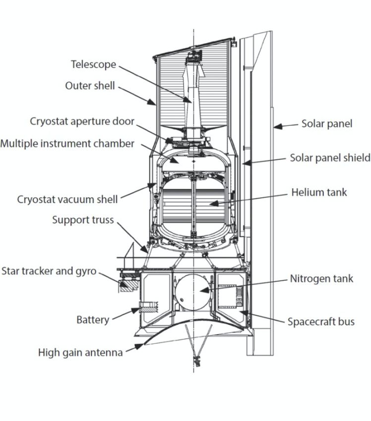
– 3.2 Instrumental sensitivity
         – 3.3 Cosmic Ray hit rate
         – 3.4 Photometric Stability

   – Section 4. Spacecraft Performance

         – 4.1 Electrical Power Generation
         – 4.2 Pointing System Performance
             – 4.2.1 Target Acquisition
             – 4.2.2 Mapping the sweet-spot
             – 4.2.3 Improving Pointing Stability
         – 4.3 Angular Momentum Management

1.1 Description of the
Spitzer Space Telescope
    NASA launched Spitzer into an Earth-trailing solar orbit in August, 2003, as a cryogenic tele-
scope cooled by liquid helium and radiation to space. Table 1 summarizes for the readers the key
properties of the Spitzer mission, and Figure 1 shows a cutaway view of the observatory as flown.
In considering these properties and the material below, readers should bear in mind that Spitzer
was highly constrained in the 1990s, both in mass/volume by the required Delta launch vehicle
and by NASA mandate to keep the cost through launch under $500M [it eventually grew to about
$750M, including launch vehicle]. These constraints dovetailed nicely with the characteristics of
the warm-launch, solar-orbiting mission which emerged as the optimum design solution, providing
the most science per dollar. As exemplified by the discussion below of the Warm Mission, these
cost constraints meant that not all conceivable analyses and design trades could be carried out.

                                                2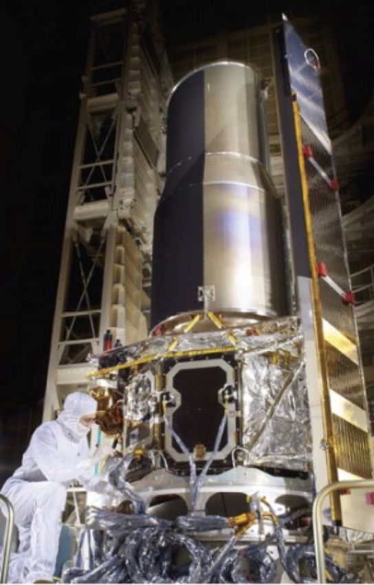
Parameter                                                           Value
              Total observatory mass at launch                                   861 kg
              Dimensions (height×diameter)                                    4.5×2.1 m2
              Average operating power                                            375 W
              Solar array generating capacity at launch                          500 W
              Nitrogen reaction control gas at launch                          15.59 kg
              Estimated reaction control gas lifetime                           17 years
              Mass memory capacity                                             2 Gbytes
              Telescope primary diameter                                         0.85 m
              Telescope operating temperature                                  5.6–13 K
              (Depending on instrument in use)
              Superfluid helium at launch                                       337 L
              Estimated nominal cryogenic lifetime                          5.6–6.0 years
              As-commanded pointing accuracy (1σ radial)                        < 0.500
              Pointing stability (1σ, 600 s)                                   ≤ 0.0300
              Maximum tracking rate                                            1.000 s−1
              Time to slew over ∼90°                                           ∼8 min
              Data transmission rate                                      2.2 megabytes s−1
              (high-gain antenna up to 0.58 AU from the Earth)
              Command communication rate                                    2 kilobytes s−1
                      Table 1 Top-level observatory parameters for the Cryogenic Mission
                                                      1

1.2 Cryogenic and Warm Missions
Following depletion of the initial cryogen load in 2009, the Spitzer telescope and instruments
warmed up to the point where only the two shortest wavelength imaging channels remained opera-
tional. Spitzer operated in this Warm Mission mode very successfully until the mission was retired
in early 2020. The development team realized from the first that the cryo-thermal architecture,
with its heavy reliance on radiative cooling and the use of the telescope outer shell as a thermal
boundary, would probably support the Warm Mission. However, it is important to note that NO
resources were expended during the Spitzer development to optimize or prepare the system for the
Warm Mission. Discussing the Warm Mission would inevitably distract the design/development
teams, who were fully occupied with completing the Cryogenic Mission. In addition, the cost
constraints did not make room for significant work on the Warm Mission. In NASA jargon, the
Cryogenic Mission was the Prime Mission, and the Warm Mission was the Extended Mission.
The Spitzer experience clearly shows that the best guarantee of a successful Extended Mission is
careful work on the design and development of the Prime Mission.

1.3 Spitzer’s Orbit
Unlike an observatory in Earth orbit or at L2, Spitzer had to address a separate set of challenges
arising from the fact that, in the Earth-trailing solar orbit, the spacecraft, launched 25 August 2003,
drifted away from the Earth at about 0.1 AU per year, reaching a distance of 1.75 AU at the time
of the end of the mission in January, 2020. These challenges, discussed in detail in Ref. 3, arose

                                                      3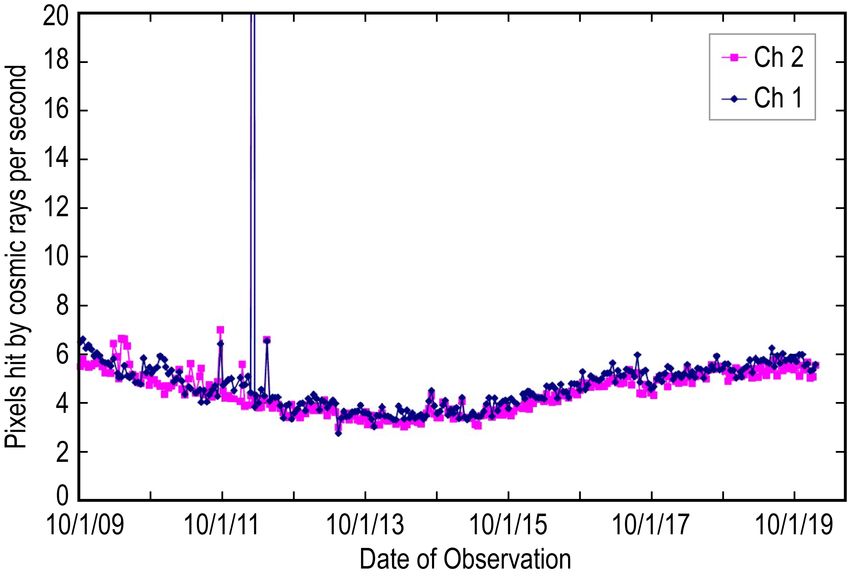
Fig 1 Cutaway view of the Spitzer observatory.2 The dust cover atop the telescope tube was jettisoned a few days after
launch, and the cryostat aperture door was opened shortly afterwards to admit infrared radiation into the instrument
chamber. See papers listed in the appendix for a detailed discussion of the in-orbit checkout for Spitzer.

from several considerations. The first was the reduced data downlink rate - from 2.2 Mbps early in
the mission to 0.55 Mbps at the end - which was a consequence of the increased distance of Spitzer
from Earth. This was compounded by the fact that Spitzer’s fixed solar panel was optimized for
solar incidence angles no greater than 30 degrees. During the Cryogenic Mission, the incidence
angle was always below 30 degrees, and during the Warm Mission, the incidence angle was always
kept below 30 degrees while Spitzer was observing. However, because Spitzer downlinked through
an antenna fixed to the bottom of the spacecraft, the communication geometry required larger solar
incidence angles during the Warm Mission, reaching 55 degrees at the end of the mission. This
had implications for battery utilization and recharging and led to solar illumination of structures
at the lower end of the spacecraft not originally planned to be in direct sunlight. In addition,
elements of the fault protection system had to be over-ridden to allow the use of such large off

                                                          4
sun angles without tripping fault protection limits. This had to be done as part of the setup for
each download; following the download the system was restored to its original configuration so
that the fault protection would still be operational. Fortunately, the spacecraft engineering team
at Lockheed-Martin, working with the mission operations team at the Jet Propulsion Laboratory
and the science planners at the Spitzer Science Center, found a solution which met all of these
constraints, at the cost of some operational flexibility as only a limited number of data-taking
modes were allowed. Thus Spitzer was able to operate with efficiency ∼90% up to the end of
its mission in January 2020. (Efficiency is defined as (time spent on science, calibration, and
slews)/(wall clock time). We will not address these issues in greater detail: We anticipate that the
much larger detector arrays anticipated for future missions, as exemplified by JWST, Euclid and
Roman, will inevitably point future missions to L2, where none of these problems need arise, and
where the thermal and sky-visibility benefits of the solar orbit remain. We did consider L2 instead
of the solar orbit for Spitzer but felt that the mass, cost, complexity and risk (to our cold surfaces)
of the station-keeping made it less attractive than the solar orbit for the heavily constrained Spitzer.
It is instructive with regard to the previous discussion to note that Spitzer’s orbit had an ec-
centricity of 0.0113 and a period of 373.1 days, slightly longer than an Earth year. Spitzer was
inserted directly into this orbit by a final rocket burn which ejected it from Earth’s orbit. It was this
difference to the Earth’s orbit which caused Spitzer to fall further behind the Earth every year. The
Spitzer orbit was chosen both to assure that the observatory was not in danger of falling back to
Earth, and, more importantly, to allow Spitzer to escape rapidly from the Earth’s heat load so that
the radiative cooling could proceed. No station keeping was required in this orbit, and the cold N2
gas system described below was used only for momentum management, not for orbit maintenance.
Finally, we point out that Spitzer was a robust and reliable spacecraft. Over the 16+ year mission,
Spitzer averaged only slightly more than 1 safing or standby event per year. Fewer than 4 days/yr
were lost to these events.
2 THERMAL CONSIDERATIONS
2.1 Thermal System Design and Performance – Use of Radiative Cooling
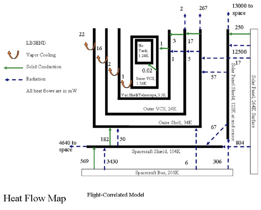
The discussion below will refer repeatedly to the heat flow diagram for the cryogenic mission
shown in Figure 2. Paul Finley at Ball Aerospace developed this model, which represents a corre-
lation of the on-orbit performance of the thermal system early in the Cryogenic Mission with the
prelaunch thermal model. Unfortunately, no comparable heat flow diagram exists for the Warm
Mission, but some of the elements of Figure 2 bear directly on the thermal performance of the
Warm Mission.
Spitzer was launched with its cryostat containing 337 liters (49 kg) of superfluid liquid helium,
which cooled the instruments and the telescope. Spitzer operated in this Cryogenic Mission mode
until mid-2009, utilizing all three science instruments and observing at wavelengths between 3
and 180 µm. When the helium supply was exhausted in mid-May of 2009, the system warmed
up to a level where only the two shortest wavelength arrays of the Infrared Array Camera (IRAC)
instrument, operating at 3.6 and 4.5 µm, had low enough dark current to be useful for scientific
observations. This phase, referred to below as the Warm Mission, lasted until the observatory was
turned off in January, 2020. Here we discuss the thermal history of key components of Spitzer’s
thermal system over the entire 16+ yr mission. Figures 1 and 2 will illuminate this and the fol-
lowing discussions. Note that, unlike the previous Infrared Astronomical Satellite (IRAS) and
5Fig 2 Ball Aerospace thermal model.1 Heat input is solely from insolation on the solar panel. Cooling of the cryogenic
telescope assembly is accomplished by radiation and vapor cooling. Heat is transferred through the system along the
paths indicated by the arrows by radiation (dashed blue arrows), conduction (solid green arrows), and vapor cooling
(broad orange arrows). The equilibrium temperatures for the various observatory components are given for the case
when the cryogenic telescope is operating at 5.5 K. The model assumes a focal-plane heat dissipation of 4 mW and an
insolation of 5.3 kW. Courtesy of Ball Aerospace/JPL-Caltech.
Infrared Space Observatory (ISO) missions, which launched with the telescope inside the cryostat,
the Spitzer telescope was launched warm and cooled on orbit, making maximum use of radiative
cooling to lose energy to the coldness of space.
Some idea of the overall efficiency of the Spitzer cryogenic system is given by the following:
After the loss of helium due to blowdown and on-orbit cooling, the observatory entered its final
stages of in-orbit checkout on October 10, 2003, carrying 43.4 kg of liquid helium, down from
the 49 Kg present at launch. This lasted through May 15, 2009, a total of 2030 days, so that
the helium was boiled away at a rate of 0.24mg/sec. The corresponding average heat load to the
helium bath was 5.1 mW, consistent with the power dissipated at the focal plane by the instruments
and make-up heaters. In comparison, IRAS carried 73 kg of liquid helium and had a lifetime, in
low Earth orbit, of 10 months, as opposed to the over 5.5 years achieved by Spitzer with 42.5 Kg
of liquid helium. IRAS’s helium usage was dominated by parasitic heat conducted and radiated
6inward from the warm outer shell of the cryostat; Spitzer, using radiative cooling in the thermally
advantageous heliocentric orbit to cool the telescope outer shell, had helium utilization dominated
by the much lower power level needed to operate the arrays and the make-up heater used to control
the helium bath temperature, and thus the telescope temperature as well (see section 2.5).Although
improvements to the Spitzer thermal design could be contemplated, we emphasize that the heat
load to the helium bath was dominated by the unavoidable [though minimal] power demands of
the focal plane instruments. Thus the cryogenic lifetime was in fact determined by the amount of
helium remaining after launch and initial cooldown. The size of the cryostat was limited by the
constraints discussed above, so the only design improvements which could significantly increase
the cryogenic lifetime would be ones which minimized the amount of helium used in the initial
mission phases, and none have been suggested.
2.2 The Solar Panel
We discuss the thermal history of key elements of the Spitzer thermal/cryogenic system, starting
at the outside and working inward. The photograph in Figure 3 shows the elements of the thermal
system external to the telescope. Spitzer was optimized for studies at infrared wavelengths, which
required that the telescope, its baffles, and the instruments be cooled to below 10 K. To achieve
this within the cost and mass constraints imposed programmatically, the telescope was designed
and operated so as to make maximum use of radiative cooling as illustrated in Figure 2. During
the Cryogenic Mission, the fixed solar panel (cf. Fig 3) was always oriented to shade the telescope
outer shell and the spacecraft from the sun, and the anti-solar side of the outer shell was painted
black to enhance its radiative cooling power. The solar panel assembly was provided by Lockheed-
Martin as part of the spacecraft. Most of the rest of the flight system including the solar panel
shield, the spacecraft shield, the outer shell and the structures within it, as well as the Infrared
Spectrograph (IRS) and Multiband Imaging Photometer (MIPS) instruments, was provided by Ball
Aerospace. Goddard Space Flight Center provided the third instrument, the Infrared Array Camera
(IRAC) which was the only instrument in use during the Warm Mission and features prominently
in this paper.
To understand the thermal performance of Spitzer, we start at the solar panel, which absorbs and
redistributes all the power – in the form of both electrical and thermal energy – coursing through
the Spitzer system. The solar panel was divided into two sections. The lower portion, consisting
of two 330 × 72 cm panels arranged in a chevron arrangement (Figure 3) was 60% covered with
11 mil GaAs/Ge solar cells with 18% efficiency at launch, similar to those which were flown on
the Iridium spacecraft. The solar cells provided more than the ∼375W average operating power
required by Spitzer throughout the mission. An aluminum upper section extended the chevron
an additional ∼160 cm above the active section of the solar panel and shaded the upper section
of the telescope outer shell from direct sunlight. Thus the solar panel served as both sunshade
and electric power generator. The sun-facing side of this extension and the regions of the lower
section not occupied by solar cells were covered with second-surface aluminized Teflon with an
absorption/emissivity ratio of 0.26/0.80, designed to minimize the temperature of the solar panel.
Figure 4 shows the average temperature of the active lower segment of the solar panel as a
function of time throughout the Spitzer mission. The temperature shows a gradual increase in
time, superposed on a periodic annual variation due to the eccentricity of Spitzer’s orbit. Over the
16+ year mission the temperature of the active portion of the solar panel increased from 338 to 344
7Fig 3 The assembled Spitzer observatory being prepared for thermal vacuum testing at Lockheed Martin in Sunnyvale,
CA. The photograph illustrates the key features of the thermal control system up to and including the outer shell of
the telescope. These include the chevron-shaped solar panel, the solar panel shield immediately behind it, and the
telescope outer shell, with its anti-solar side painted black to maximize its infrared emissivity. Also visible between
the spacecraft and the outershell is the spacecraft shield which isolated the outer shell from the spacecraft. Credit:
NASA.
K, corresponding to an increase in absorbed power by (344/338)4 − 1 = 0.073, or 7.3%, because
the solar panel cools principally by radiation. This increase is attributed by Ref. 4 to “unsurprising
degradations in thermal coatings on the solar panel”. Similar increases in temperature are seen in
other long-lived space systems; and attributed, as suggested above, to degradation of the solar panel
materials by the effects of unfiltered solar ultraviolet light and the energetic particle environment
in space. In the case of Spitzer, the increased solar panel temperature is accompanied by a drop in
the electrical output (discussed below) which may also be attributed to degradation of the optical
properties of the solar panel materials.
2.3 The Solar Panel Shield and the Outer Shell
The solar panel shield lies between the solar panel and the outer shell described below (see Figure
3). Structurally, the solar panel shield and the outer shell are constructed of lightweighted alu-
minum honeycomb cores with thin face sheets. The solar panel shield and the solar panel are stood
off from the spacecraft by Gr/CE struts and not physically attached to any portion of the telescope
outer shell. The surface finishes are chosen to control heat flow – low emissivity surfaces, such as
the facing sides of the outer shell and the solar panel shield, are coated with co-cured aluminized
Kapton. By contrast, as shown in Figure 3 the space facing back half-cylinder of the outer shell
is coated with a proprietary Ball black paint,5 which gives it very high emissivity even at the low
8Fig 4 The average temperature of the lower, solar cell-containing portion of the solar panel vs. time over the entire
Spitzer mission. The annual periodicity seen in this and the other temperature data reflects the eccentricity of Spitzer’s
orbit.
temperatures achieved on orbit. As shown in Figure 2, the solar panel shield coupled to the solar
panel primarily through radiation, with only 2% of the heat transferred by conduction. The solar
panel shield loses most of this energy by radiation to space, thereby greatly reducing the heat load
on the outer shell. Multilayer insulation [MLI] thermal blankets were used to reduce the temper-
atures of the solar panel shield and the spacecraft shield (Figure 3), which were adjacent to the
telescope outer shell, to 122K and 104K, respectively. One blanket lay between the solar panel and
the solar panel shield, while the other was positioned below the spacecraft shield.
All of the energy which found its way into the critical telescope/cryostat structure passed
through the outer shell. Thus the telescope outer shell was a critical node in the thermal system,
as it set a thermal boundary for the telescope and the cryostat, which sit within it. The cryostat
contained the liquid helium tank and the instrument chamber, which is thermally coupled to the
helium tank and not to the cryostat vacuum shell. On orbit, the heat input to the telescope outer
shell, a structure ∼3m in length and ∼1.2 m in diameter, was about 310 mW, which is one part in
17,000 of the 5.3 kW striking the solar panel. The outer shell was heated approximately equally
by radiation and conduction (Figure 2). The radiation was from the solar panel shield and from
the spacecraft shield, which lay between the spacecraft and the outer shell. The conduction was
from the mechanical and electrical connections between the spacecraft and the outer shell; the mi-
crocables passing inwards to the cryostat and the instruments were heat sunk to the outer shell via
its supporting truss of low conductivity gamma-alumina struts. The outer shell lost energy through
radiation to space, and, to a much lesser extent, by conduction inward. Because the radiative and
conductive heat loads into the outer shell are comparable, the system was “well- balanced” in a
thermal sense. During the Cryogenic Mission, the heat conducted inward was carried away by the
last stages of vapor cooling provided by the evaporated helium as it left the system through a low-
thrust valve. It is important to note that the heat loads to the outer shell did not vary dramatically
between the Cryogenic and Warm Missions beyond the gradual increase implied by the thermal
9histories shown in this paper.
Fig 5 Spitzer outer shell temperature vs. time over the entire Spitzer mission. The discontinuity in 2009 reflects the
exhaustion of the liquid helium and the start of the Warm Mission, when vapor cooling was no longer available. The
oscillations in temperature seen before this reflects the variation in vapor cooling resulting from the helium utilization
strategy described in the text.
As the power absorbed by the solar panel increased over the mission, a corresponding rise
occurred in the temperature of the outer shell. Figure 5 shows the outer shell temperature as a
function of time over the entire 16+ year Spitzer mission. The step upward rise in temperature by
about 0.5K seen in 2009 marks the exhaustion of the liquid helium and the start of the Warm Spitzer
mission. At this point, the absence of vapor cooling allowed the outer shell to warm slightly. It also
allowed more heat to be conducted inwards to the structures within the outer shell. These struc-
tures warmed far above the temperatures characteristic of the Cryogenic Mission. The outer shell
temperature continued to rise slowly after this, as expected from the rising temperature of the solar
panel which let more heat into the Spitzer system. We also see the annual variation of temperature
due to the eccentricity of Spitzer’s orbit superposed on this long term trend. The relatively large
fluctuations in temperature prior to helium exhaustion in mid-2009 reflected fluctuations in the
amount of helium gas evaporating in the cryostat and hence in the cooling power of the escaping
helium vapor, and, again, in the temperatures of the structures interior to the outer shell. These
periodic fluctuations result from the helium utilization strategy discussed below. Starting after he-
lium depletion in mid-2009, however, this cooling path was no longer in effect, but the design and
operational features which enabled radiative cooling during the Cryogenic Mission were still in
place. These features kept the outer shell temperature below 36K at the start of the Warm Mission,
maintained entirely passively.
10Note that the envelope of the temperature fluctuations prior to mid-2009 show that the temper-
ature rise began immediately after launch.4 The increase in outer shell temperature mirrored the
increase in solar panel temperature. The data in Figure 5 show an increase in temperature from
∼35.3 to ∼36K during the Warm Mission. In order to isolate the performance of the radiative
cooling system external to the outer shell, we extrapolate the data back to the start of the mission
and remove the offset due to the loss of vapor cooling. The envelope of the curve suggests perhaps
another 0.4 degree increase in temperature would have been recorded. Thus the power radiated
by the outer shell in this slightly fictional scenario increased by (36/34.9)4 − 1 = 13%. Absent a
complete thermal model, this can be taken as an upper limit for the degradation in the performance
of the radiative cooling alone, because some of the increase must be simply in response to the
increased temperature of the solar panel. Note that the outer shell loses energy predominantly by
radiation. In reality, of course, the power radiated by the outer shell increases by closer to 20%
when the effects of the loss of the vapor cooling are taken into account. Because of the factor of
10 difference in the temperatures of the two systems, this 20% increase in the power radiated by
the cold outer shell is not inconsistent with the 7% increase in power radiated by the much warmer
solar panel.
2.4 The Telescope
The telescope optics and metering structure were fabricated of hot isostatically pressed beryllium.
Beryllium was chosen because of its favorable strength to weight ratio and its mechanical stability
at low temperature. The optics were polished but not coated. The telescope and its barrel baffle
lay within the outer shell and were surrounded by a vapor cooled shield which intercepted en-
ergy conducted and radiated inward from the outer shell. The telescope was thermally anchored
to the exterior vacuum shell of the cryostat which, in turn, was cooled by the helium boil-off.
Two vapor cooled shields provided additional thermal isolation of the helium tank and its associ-
ated instrument chamber from the cryostat vacuum shell. The instrument chamber contained the
three instruments and the Pointing Calibration and Reference Sensor (PCRS), discussed further
below. As the helium boiloff rate was varied according to the strategy described below, the cryo-
stat outer shell and the telescope temperatures varied to meet the needs of the instrument in use.
This scenario accounted for both the low temperature of the primary mirror and the temperature
fluctuations seen during the Cryogenic Mission prior to mid-2009 (Figure 6). Except for the detec-
tors, the instrument hardware was thermally anchored to the helium tank and would rise and fall
in temperature very slightly as the bath temperature changed. During the Cryogenic Mission, the
InSb and Si:As IBC detectors used below 40µm were thermally stabilized at temperatures above
the enclosure temperature, while the Ge:Ga photoconductors in the MIPS instrument, which had
to operate below 2K, were thermally strapped directly to the helium bath.
During the Cryogenic Mission, the instrument temperature varied slightly due to the helium
utilization scheme described below. No effects on the instrument optical performance were seen
as a result of these changes. More tellingly, because of the thermal stability of beryllium, it was
neither planned nor necessary to refocus the telescope following the transition to the Warm Mis-
sion, during which the telescope temperature shifted upward from ∼10K to ∼25K.6 Over a larger
temperature change, it was noted during IOC that the position of the telescope focus stabilized to
within 0.01 mm once the telescope temperature fell below ∼50K.
11During the Warm Mission, the heat load applied within the cryostat, a combination of power
required to stabilize the two IRAC arrays in use and the power dissipated in reading the arrays out,
was constant with time at a level of 1.4 mW. The effects of the increasing outer shell temperature
and its annual variation are just visible in the telescope temperature, which was stable at 26-to-27
K throughout the Warm Mission (Figure 6). The tight mechanical coupling of the telescope, the
cryostat, and the barrel baffle suggest that all structures within the vapor cooled shield were at
about the same temperature, and these interior structures remained at ∼26K by radiating about
20 mW into space through the open end of the outer shell. This suggests that, in addition to
the 1.4 mW dissipated within the cryostat by the IRAC arrays, a bit more than an additional 20
mW was conducted or radiated from the outer shell through the shield and into these interior
structures. Although a detailed thermal model for Warm Spitzer does not exist, this lies in the
range of the conductive and radiative loads into the interior of the outer shell seen in the heat flow
diagram (Figure 2). It is important to realize that these loads on the outer shell should be about the
same in the Warm Mission, but they now warmed the telescope because the cooling effect of the
evaporating helium gas was no longer present to counteract them.
Fig 6 Spitzer primary mirror temperature vs. time over the entire Spitzer mission. The fluctuations in temperature
seen prior to the start of the Warm Mission in mid-2009 reflect the helium utilization strategy described in the text.
2.5 Maximizng the cryogenic lifetime of Spitzer
Spitzer operated only one instrument at a time (typically for a one-week campaign), as appropriate
for a system where the cryogen boil-off rate was set by the power dissipated by the instruments
within the cryostat. If two instruments were in use simultaneously, the helium would have been
used at a correspondingly higher rate, shortening the mission and reducing the time available for
12scientists to plan future observations based on initial results. This single-instrument mode enabled
the following strategy for maximizing the cryogenic lifetime of Spitzer.
The fluctuations in the primary mirror temperature during the Cryogenic Mission (Figure 6)
reflect a tailoring of the mirror temperature to the needs of the instrument being used. Through
the use of a heater which increased the rate at which helium was evaporated in the cryostat, the
telescope was kept cold enough (5.5K) for natural-background-limited operation when the long
wavelength MIPS instrument was in use. The heater was turned off and the telescope temperature
was allowed to drift upwards when the shorter wavelength instruments- IRAC and IRS - took over.
This tailoring increased the cryogenic lifetime of the system by at least six months over an approach
in which the mirror temperature was always kept at 5.5K. It may have application to future missions
which carry expendable cryogens and is described in detail by Ref. 7 and summarized by Ref. 8.
2.6 Integration, test, and verification of the cryo-thermal system
A pre-launch test of the performance of the cryo-thermal system was necessary to assure that
Spitzer would meet its requirement of 2.5 years cryogenic lifetime (the pre-launch goal was five
years). The NASA mantra “Test as you Fly” was, unfortunately, not applicable to tests of Spitzer’s
cryo-thermal system due to the impracticability of replicating the very low thermal background of
space, together with solar insolation on one side, in any test chamber large enough to accommodate
the entire Spitzer observatory. Instead, we broke this verification into two parts, with the boundary
at the outer shell. The reasoning was simple: In flight, all heat input into the telescope, instruments,
and cryogen system was routed through the outer shell. Thus the telescope temperature and the
helium flow rate would depend only on the outer shell temperature and not directly on any external
heat sources. The thermal performance of the structures within the outer shell was to be tested in
the thermal balance test at Ball Aerospace, carried out with fixed outer shell temperatures.
The thermal performance of the hardware external to the outer shell, which established the
outer shell temperature, was evaluated as part of the system level thermal vacuum test, which
was carried out at much higher temperatures. In neither case did the test conditions faithfully
replicate the on-orbit conditions, so much of the test effort was devoted to validating the models
which were to be used to understand the test results and to extrapolate from the test to the orbital
environment. These tests evaluated not only the design of the thermal system but also the quality
of the workmanship involved in its assembly.
Ref. 9 describes the low temperature thermal test and verification of the outer shell and its
interior components. The tests were carried out in a chamber at Ball Aerospace with walls cooled
by liquid nitrogen, with the telescope, the cryostat, and the instruments assembled for launch within
the outer shell (the thermal test was done concurrently with an end-to-end optical test described
below). The outer shell was shielded from a direct view of the chamber walls by extensive thermal
shields and blankets. The original intent of the test was to set the outer shell temperature at both
nominal and worst-case values expected on orbit and to measure the telescope temperature and the
helium flow rate in each case. The outer shell temperature was to be controlled by circulating cold
helium vapor through a cooling loop at the base of the outer shell. This cooling loop was included
in the design for just this purpose, illustrating the importance of outlining the test strategy during
the design phase for a complex, difficult to test, system like Spitzer.
However, data taken during the initial cool down showed that the heat load on the vacuum shell
of the cryostat, which lay interior to the outer shell and was mechanically and thermally coupled
13to the telescope, was 5 to 10 times the 5-to-10 mW expected on orbit. This uncontrolled power
was small compared to the potential test induced heat input from radiation or solid or gaseous
conduction (there were four separate cooling loops bringing in helium from vessels outside the test
chamber); for example, a blackbody at 273K radiates about 30 mW/cm2 . The challenge detailed
in Ref. 9 was to separate the environmental or test-induced heat loads from those intrinsic to the
system; only the latter would be present in flight. To do this, the authors did a careful audit of the
possible test-induced heat loads, which are described in detail in Ref. 9, to determine which were
credible, and incorporated them into a thermal model of the test configuration which also included
the parameters characterizing the thermal performance of the flight system. They identified nu-
merous possible sneak heat paths, including, for example, radiation down the pipes used in cooling
loops which carried liquid helium from outside the test dewar into the outer shell. Following cor-
rection of these known problems, there were quite a few parameters to be evaluated, and the long
thermal time constant of the system made it impractical to test each separately. Instead, a series of
8 separate energy balance cases, each with a different set of environmental and system parameters,
were carried out and analyzed in detail. Because the system never reached thermal equilibrium
during these tests, much of the analysis focused on the transient behavior of the system, which was
predicted by the thermal model. The transient behavior reflected the thermal coupling between
various system elements, which was central to the on-orbit performance. In short, the purpose
of the telescope thermal balance test became validation of the thermal model rather than actual
demonstration of flight performance.
This painstaking work succeeded in separating the test artefacts – which were still dominant
- and in predicting on-orbit behavior. It set the stage for the observatory level thermal balance
test of the assembled spacecraft, carried out in a large chamber at Lockheed Martin, Sunnyvale,
and shown in Figure 3. As was the case for the test of the outer shell and its interior systems,
described above, it was not possible during the observatory thermal balance test (which had other
objectives in addition to supporting an estimate of the cryogenic lifetime) to replicate the boundary
conditions which the observatory would encounter in space. Instead, the analysis focused on three
time windows, spread over about three days, during which temperatures of key system elements
were measured as the observatory cooled down. Prominent among the elements investigated were
the spacecraft shield and the solar panel shield, because a key objective was to test whether these
components, which were expected to dominate the radiative and conductive loads on the outer
shell during flight, could adequately isolate the outer shell from the heat of the solar panel and the
spacecraft. Of course, the outer shell temperature was monitored as well. In a similar spirit to that
of the outer shell test described above, the analysis focused on the changes in temperature from
one time window to another rather than on the actual temperatures, which were greatly influenced
by environmentally-induced heat loads.
Comparison of the actual flight performance with the prelaunch predicts based on the tests de-
scribed above shows that the latter were remarkably accurate. The analysis10 of the prelaunch data,
following the thermal balance test, showed that even the worst case (when all thermal parameters
were stacked up with their least favorable values), yielded a cryogenic lifetime of 3.1 years, consid-
erably longer than the 2.5 year requirement, while the nominal cryogenic lifetime was predicted to
be 5.1 years. This lifetime analysis assumed that the telescope was constantly cooled to its lowest
required operating temperature of 5.5K.
It was already apparent that the adaptive cryogenic utilization scheme described above would
increase the lifetime by 5 to 10%, leading to a more realistic lifetime prediction of 5.4 to 5.6 years.
14These pre-launch predictions agreed extremely well with the actual on-orbit cryogenic lifetime
of just under 5.7 years. Similarly, the predicted temperatures9 of specific components during the
Cryogenic Mission agreed very well with the on-orbit data. Most importantly, the outer shell
temperature was predicted to be 32K, very close to the observed value of 34-to-34.5K (Figure 5).
Finally, when the thermal model was adjusted following launch to fit better the actual tempera-
tures measured during the Cryogenic Mission, it predicted temperatures during the Warm Mission
of 24K for the telescope and 36K for the outer shell (P. Finley, private communication). Again,
these predictions were in good agreement with the measured values shown earlier (Figs 5 and 6).
It is noteworthy that almost 20 years ago the state of the art thermal modelling led to very accu-
rate predictions of the on orbit behavior of a complex system which utilized both radiative and
cryogenic cooling. The performance and predictability of Spitzer’s radiative cooling approach has
been important in reducing the risk of the use of radiative cooling in other NASA missions, such
as JWST and SPHEREx.
In summary, the performance of the Spitzer cryogenic system on orbit was remarkable. It is a
tribute not only to the careful design of the system by our partners at Ball Aerospace, but also to
the extreme care with which it was assembled and tested. For lessons learned from this experience
we refer the readers to the publications by the Ball group4, 9–11 as well as the more general lessons
learned analysis of Ref 12. Two lessons which stick out, however, are the following: 1) For a
complex cryo-thermal test such as that undertaken for Spitzer, the design and fabrication of the test
configuration and other GSE need as much care and attention as was given to design and fabrication
of the flight system; and, 2) It is important to remember that for systems like Spitzer for which the
on-orbit thermal environment cannot be duplicated in the lab, the thermal balance tests can be used
to validate the system thermal model, which can then be used with greater confidence to predict
the on-orbit behavior. In this modelling and validation, it may be found that tests constructed and
instrumented to permit analysis of the transient behavior of the system are equally valuable, and
considerably easier to implement, than those which rely on reaching a steady state temperature,
which may take a prohibitively long time.
3 Payload Issues
3.1 Optical System Verification and Focus Adjustment
Spitzer used an all-beryllium 85-cm diameter f/12 Cassegrain telescope which illuminated a focal
plane ∼30 arcmin in diameter. The focal plane housed pickoff mirrors which fed the modules of all
three Spitzer instruments as well as the PCRS. The telescope was body pointed to place the target
of interest onto the pickoff mirror, and hence the entrance aperture, of the instrument/module to be
used for a particular observation. This design required that the instrument modules be confocal;
this was achieved by design and test on the ground and verified on-orbit. The telescope with the
instruments installed underwent optical test and verification at cryogenic temperature in the large
cryogenic test chamber at Ball Aerospace. These tests were simultaneous and interleaved with the
thermal verification tests described above. A standard double-pass test using a cold flat mounted
above the telescope, and a short wavelength infrared source placed at the telescope focal plane by
Ball for just this purpose, illuminated the IRAC arrays at 3.6 and 4.5 µm. The test validated the
end-to-end image quality of the system, discussed further below. It also allowed the Spitzer team
to use the focus mechanism, which was part of the secondary mirror assembly, to set the focus
at the estimated position expected for the zero-gravity post-launch configuration. The primary
15mirror was polished to have the right configuration for its cryogenic performance by measuring
the distortions in the figure at cryogenic temperature and polishing the inverse of the measured
deviations into the mirror at room temperature. Following the warm polishing of the mirror and
an initial cryogenic test, one additional polishing cycle was carried out following this approach,
after which a second cryogenic test confirmed that the mirror met specifications. Further details
concerning the design, fabrication, test and performance of the optical system are given by Ref. 1.
The approach taken on orbit to determine and then set the optimum position for the secondary
mirror may be relevant to future space observatories. The focus mechanism provided motion only
along the optical axis and was robustly designed and electrically redundant. Nevertheless, there
was an understandable reluctance to carry out a traditional focus sweep which would require many
activations of the focus mechanism at cryogenic temperature. Instead, a group led by Bill Hoff-
mann from the University of Arizona developed a technique for determining focal position by look-
ing at the variation of image quality across the combined ∼5 by 10 arcmin field of view of the two
short wavelength IRAC arrays at 3.6 and 4.5 µm. This technique, described by Ref. 13 and summa-
rized by Ref. 8, was validated through a double-blind simulation on the ground14 and successfully
applied on orbit. A series of on-orbit measurements showed that the position of the telescope focus
had stabilized to better than 0.01mm once its temperature fell below ∼50K,1 as was expected from
the thermo-mechanical properties of beryllium and the other materials in the mechanical assembly.
At this point, the analysis13 showed that the telescope focus lay 1.8mm above the nominal focal
plane established by the instrument entrance apertures. A small test move of the focus mechanism
verified the direction of motion. Then a larger motion of the secondary mirror brought the focus
position within the required range. The telescope optics alone provided an image FWHM of ∼1.45
arcsec15 at the center of the 3.6 and 4.5 µm arrays. However, when the effects of the instrument
optics and array pixelization are considered, the images in the reduced data have FWHM 1.6-to-
2” ( https://irsa.ipac.caltech.edu/data/SPITZER/docs/irac/iracinstrumenthandbook/5/). This image
quality has supported Spitzer studies of highly redshifted starlight from galaxies in the distant
Universe.
3.2 Instrumental Sensitivity
With its very cold optics and careful stray light baffling, the Spitzer observatory achieved photo-
metric sensitivities close to the limits imposed by natural backgrounds in its broad band imaging
instruments. Figure 7 shows a comparison of the measured Spitzer instrument sensitivity com-
pared to the natural background limit due to the zodiacal emission in the direction of the North
Ecliptic Pole. The calculated natural background limit includes the measured Spitzer instrumental
optical throughput as detailed in the figure caption, but assumes otherwise perfect instruments with
noiseless detectors and 100% on-source observing efficiency. The natural background limit also
assumes an ideal instrument with a large number of small noiseless pixels that can capture and
properly weight the point spread function. In the case of the Spitzer instruments the pixels are
larger than this ideal (to reduce the effects of excess noise that could arise from a large number
of real pixels) - which leads to excess sky background, and thus leads to less sensitivity compared
to a perfect instrument. In practice, even the zodiacal background limit will actually be degraded
by galactic cirrus emission and source confusion, especially at the longer wavelengths. This is
readily apparent in the figure where the measured sensitivity deviates most strongly in the MIPS
long wavelength bands at 70 and 160µm.16 We feel that Figure 7 and the accompanying discussion
16show that we can build instruments fully capable of exploiting the low backgrounds of the space
environment.
Fig 7 Achieved Spitzer point source sensitivities (solid lines, 1σ in 500 sec)2 compared with estimates of fundamental
limits imposed by the zodiacal background. The short vertical lines under each instrumental bandpass show the
zodiacal background-limited NEFD estimate for the bandpass, assuming noise from the zodiacal light in an annual
average sightline viewing the north ecliptic pole. Note that the achieved performance is closest to the background
limit in the 8-to-24µm range were the background is at is brightest.
The background couples in both polarizations with a square bandpass of the plotted width and
total transmission (including detector absorption efficiency) of 0.44, 0.42, 0.14, and 0.30 for IRAC
bands 3.6, 4.5, 5.8, and 8.0 µm, 0.6, 0.18, and 0.15 for MIPS 24, 70 and 160 µm, and 0.65 for
the IRS blue peak-up array (PU B) at 16 µm. Perfect detectors which add no noise other than
generation-recombination noise are assumed throughout. The sensitivity achieved by MIPS is
degraded below the zodiacal limit, in part, by the effects of confusion at both 70 and 160 µm; it
is appreciable in both channels in 500 sec. The IRS short-low and long-low module sensitivities
are referred to a λ/δλ = 50 bin; the estimates adopt wavelength-independent efficiencies of 12%
and 8.5%, respectively; this is meant to include all sources of loss including slit coupling, blaze
efficiency in both polarizations, filters and detector quantum efficiency. For all, it is assumed that
the 14% obscured 85-cm√Spitzer telescope (Ageom = 0.489 m2 ) couples to a point source with 75%
aperture efficiency. The 2 photo-electron recombination penalty is included for all bands except
IRAC 1 and 2, where it does not apply.
173.3 Cosmic Ray Hit Rate
Observatories operating outside of the protection of the Earth’s magnetosphere will be more sus-
ceptible to the effects of galactic and solar cosmic rays than their better-shielded low Earth orbit
cousins. Spitzer was designed with radiation-hardened shielding and tested with an assumed radi-
ation environment, and it provided data on radiation effects in the context of a modern observatory
using infrared array detectors. We describe here the effects of solar and galactic cosmic rays on
the pixels of the 3.6 and 4.5 µm InSb arrays used by IRAC. For data processing, the number of
affected pixels in a known time interval, typically 100 sec, was tracked, using the dark-sky calibra-
tion observations taken with IRAC once per week, and was found to correspond to 4–to-6 affected
pixels per second (Figure 8) for a 256×256 pixel array of ∼ 30×30 micron pixels. The full-well
capacity was ∼ 45000 e− and the array material InSb. The threshold for inclusion in Figure 8
was that the pixels were 10-sigma outliers once all the point sources were removed from a given
frame. Multiple dithers at each pointing position allowed the identification of cosmic ray hits even
if they coincided with a point source on the sky. In most cases, only one pixel was affected at
the 10-sigma level by a particular cosmic ray. The trend observed in the IRAC data followed the
inverse of the solar cycle, as expected, with fewer particle hits during peak solar activity. The fact
that the hit rate contained the imprint of the solar cycle shows that galactic cosmic rays, rather than
solar particles, dominated the particle flux except during major solar events. These images were
also used to count the number of bad, noisy, and dead pixels.
Fig 8 Average number of pixels in the IRAC arrays affected by cosmic rays in the calibration frames taken during the
Spitzer Warm Mission.3 The array formats were 256×256 30µm-squared pixels, The spike in 2012 was due to a solar
flare.
Taking 5 pixels/second as a typical hit rate, and bearing in mind that each array consisted of
18256×256 30µm-sized square pixels, and assuming that each incident particle liberated enough
charge to register as a cosmic ray hit, the isotropic flux of ionizing particles was about 8 cm−2 s−1 .
We feel this is broadly consistent with expectations based on the observed flux of high energy
cosmic rays and energetic solar particles. It is noteworthy that the data for each of the two IRAC
arrays showed the same hit rate and the same temporal behavior. This is of course what one would
expect if the saturated pixels are attributable to externally-incident ionizing radiation. See Ref. 17
for more information about the radiation hits and discussion of other issues related to precision
Warm Mission photometry with Spitzer.
The IRAC data processing pipeline monitored all data, even that obtained during solar flares,
to apply corrections for radiation hits before the data were released to the science investigator.
Affected pixels were identified for a single observational period pointed at one part of the sky.
This usually consisted of between 20 and 1000 single frames of the same exposure time. The
data processing pipeline created a mask file that kept track of any problem pixels for each frame.
As the telescope’s field of view was dithered or scanned across the sky, an astronomical source
would be observed in multiple pixels across the array, but a cosmic ray would affect only one pixel
(typically) in one frame. When stacked by astronomical coordinates, an astronomical source would
appear in multiple frames, so an outlier is a pixel with anomalous flux appearing in only one of the
frames. Those outlier pixels were then flagged as radhits, marked in the pixel masks, and excluded
when a mosaic, or image map, of the observations was created. This aided in producing artefact-
clean images while preserving the processing history. Early in the mission, it was found that if
Spitzer were struck by a solar flare and subsequent coronal mass ejection, the number of radiation
hits measured by IRAC would rise sharply and quickly fall away. This was used to determine if
an observation needed to be retaken. This and other features of Spitzer’s response to high energy
particles, including both spacecraft and payload issues, are discussed in reference Ref. 18, which
also discusses the effects of the space environment on the solar panel performance. In addition the
position of Spitzer in its orbit allowed data on particle hits as recorded by Spitzer to be used in
partnership with data from other spacecraft throughout the inner solar system to constrain models
of Solar Energetic Particle events and Coronal Mass Ejections.19, 20
A figure of merit for the health of the arrays over time is the number of hot and noisy pixels.
These changed with time as some pixels recovered and others became hot or noisy. Pixels were
deemed noisy if the standard deviation during the IRAC measurements described above was greater
than twice that of the median for surrounding pixels and hot if the pixel retained > 50 counts (DN)
after the flux was read out. In Band 1 (the results for Band 2 are similar), the number of hot
pixels increased fairly uniformly from 80 to 200 over the course of the Warm Mission, perhaps
reflecting the increased accumulated ionizing radiation dose, while the number of noisy pixels
bounced around more randomly but generally stayed below the hot pixel count. In practice, we
found that it sufficed to update the bad pixel masks about twice per year. Dead, or non-responsive,
pixels increased from about 20 to about 35 during the Warm Mission. The effects of cosmic ray
hits were reversible, and more than 98% of pixels remained usable at end of the 16+ year mission.
A hot pixel table was separately maintained for the star tracker, which used a 512×512 CCD with
20 µm pixels and a novel “lost in space” acquisition strategy described in detail by Ref. 21. At the
end of the mission, there were 46 hot pixels listed in this table.
Note that at the Observatory level, Spitzer was protected against cosmic rays by the use of
radiation hardened components, including computer, FPGA, and opto-electronic coupler chips. It
is noteworthy that of the 19 events which caused Spitzer to enter Standby or Safe mode over the 16+
19year mission, only one could definitely be attributed to a Single Event Upset (SEU). This occurred
in February, 2009, when an SEU induced a double memory fault in the Combined Electronics unit
which served both the IRS and the MIPS Si:As and Si:Sb arrays.
3.4 Photometric Stability
The IRAC team monitored the system’s photometric stability at 3.6 µm and 4.5 µm by periodically
repeating observations of calibration stars. The calibration stars included twenty-one primary and
secondary stars chosen at the beginning of the Cryogenic Mission.22 The calibrator stars were
either K giants or A main sequence stars as it was thought that these stellar types could be well
modeled and the stars were known to not have astrophysical variations at these wavelengths. Pri-
mary calibrators were located in the continuous viewing zone at the orbit poles so an entire set of
primary stars could be observed every two weeks. These were used to determine the flux conver-
sion for each camera. The set of secondary calibrators had positions near the ecliptic plane and
therefore only two were visible at any given time. These were used to monitor the stability of the
photometry over 12-to-24 hr timescales.
We use seven primary calibrators to examine the measured responsivity over the final 8 years
of the Warm Mission (Figure 9). The calibration stars were observed with a dither pattern in
full array mode. The flux densities were measured with a radius of 3 pixels and a reference sky
annulus of 3-7 pixels. They were corrected for both the array location dependence and the pixel
phase effect (see below), Dithering to many positions and binning over all stars reduced systematics
from each of these effects. Each individual star’s measurements were normalized to the median of
all observations of that star over time before being binned together with the other calibration stars
at a given epoch to determine the median responsivity at that epoch. Error bars were calculated for
each time-bin by taking the standard deviation of the ensemble of photometric points and dividing
by the square root of the number of data points in the bin. The data at channel 1 clustered around
a median flux of 1, showing only the small variability discussed below. The channel 2 data were
comparably stable but offset in the plot for clarity. All data were processed with pipeline version
S19.2. For further details see Ref. 17.
Figure 9 shows a decline in responsivity of 0.1% and 0.05% per year in ch1 and 2 respectively,
over the final 8 years of the mission. Similar studies of the Cryogenic Mision23 show a similar rate
of drop in responsivity for the InSb arrays; unfortunately, similar data are not readily available for
the other Spitzer detectors. Other than changes in dark current or noise, which were frequently
reversible, there is no evidence of any degradation of the arrays with time. We feel that the most
likely cause of the drop in responsivity was radiation damage to the optics, which is expected in
the space environment and would cause Rayleigh scattering in the transmissive elements. Other
possibilities could be radiation damage to the band-defining filters or to the beam splitters, which
were used in reflection for IRAC bands 1 and 2. The materials used in these lenses, filters and
beamsplitters include MgF2 and ZnS lenses for the 3.6 µm band and ZnSe and BaF2 for the 4.5
µm channel. The radiation from the sky reflected off of a multi-layer dielectric beam splitter with
a Germanium substrate, and the band-defining filters were multi-layer coated Ge. Finally, the
arrays were anti-reflection coated with SiO. For more information, consult the IRAC instrument
handbook ( https://irsa.ipac.caltech.edu/data/SPITZER/docs/irac/).
The IRAC InSb arrays were thermally stabilized at around 15K during the Cryogenic Mission
and 29K for the Warm Mission, and the bias points were reset for optimum performance.6 As a
20You can also read