Optimal minimum wages - Discussion Paper
←
→
Page content transcription
If your browser does not render page correctly, please read the page content below
Discussion Paper   ISSN 2042-2695

No.1823
January 2022

Optimal minimum
wages

Gabriel M. Ahlfeldt
Duncan Roth
Tobias Seidel
Abstract
We develop a quantitative spatial model with heterogeneous firms and a monopsonistic labour market
to derive minimum wages that maximize employment or welfare. Quantifying the model for German
micro regions, we find that the German minimum wage, set at 48% of the national mean wage, has
increased aggregate worker welfare by about 2.1% at the cost or reducing employment by about 0.3%.
The welfare-maximizing federal minimum wage, at 60% of the national mean wage, would increase
aggregate worker welfare by 4%, but reduce employment by 5.6%. An employment-maximizing
regional wage, set at 50% of the regional mean wage, would achieve a similar aggregate welfare effect
and increase employment by 1.1%.
Keywords: General equilibrium, minimum wage, monopsony, employment, Germany, inequality.
JEL: J31; J58; R12
This paper was produced as part of the Centre’s Urban Programme. The Centre for Economic
Performance is financed by the Economic and Social Research Council.
We are grateful to comments and suggestions we received at workshops and conferences in Amsterdam,
Düsseldorf (UEA), Berlin, (DIW conference on the evaluation of minimum wages, minimum wage
commission conference), Kassel (Regionaloekonomischer Ausschuss), Bonn (German Economists
Abroad), London (LSE Labour workshop), Rome (Bank of Italy), the IAB (online) and in particular to
Gaetano Basso, Francesca Carta, Emanuele Ciani, Wolfgang Dauth, Gilles Duranton, Maximilian von
Ehrlich, Alexandra Fedorets, Bernd Fitzenberger, Steve Gibbons, Simon Jaeger, Philip Jung, Attila
Lindner, Andreas Mense, Guy Michaels, Henry Overman, Michael Pflüger, Hans Koster, Joachim
Möller, Gregor Singer, Michel Serafinelli, Jens Südekum, Erik Verhoef, Jos van Ommeren, Eliana
Viviano, Jens Wrona, and Atsushi Yamagishi. The usual disclaimer applies.
Gabriel M. Ahlfeldt, London School of Economics, CEPR, CESifo and Centre for Economic
Performance, LSE. Duncan Roth, Institute for Employment Research (IAB). Tobias Seidel, University
of Duisburg-Essen, CESifo, CRED.
Published by
Centre for Economic Performance
London School of Economics and Political Science
Houghton Street
London WC2A 2AE
All rights reserved. No part of this publication may be reproduced, stored in a retrieval system or
transmitted in any form or by any means without the prior permission in writing of the publisher nor be
issued to the public or circulated in any form other than that in which it is published.
Requests for permission to reproduce any article or part of the Working Paper should be sent to the
editor at the above address.
G.M. Ahlfeldt, D. Roth and T. Seidel, submitted 2022.
1 Introduction
On few questions do economists disagree so passionately as on the desirability of minimum
wages. The controversy is primarily an empirical one since there is arguably a theoret-
ical consensus that a sufficiently high minimum wage will reduce employment. That a
sufficiently low minimum wage may increase employment and welfare in a monopsonistic
labour market also seems consensual. The open policy question is which minimum wage
level maximizes employment or welfare. We develop a quantitative model that offers an
answer.
   Our approach differs from a vast literature using reduced-form methods to study em-
ployment effects of minimum wages summarized by Manning (2021) and Neumark and
Shirley (2021). Instead, we develop a quantitative spatial model with heterogeneous firms
and a monopsonistic labour market to study minimum wage effects in a spatial general
equilibrium. Our model is uniquely equipped to derive optimal minimum wage schedules.
For one thing, our model accounts for qualitatively and quantitatively heterogeneous em-
ployment responses in regions of distinct productivity (Christl et al., 2018). This allows us
to predict both regionally differentiated and aggregate employment effects. For another,
our model accounts for a broad range of minimum-wage effects that have recently been
documented in the literature, including effects on labour force participation (Lavecchia,
2020), tradable goods prices (Harasztosi and Lindner, 2019), housing rents (Yamagishi,
2021), or commuting costs (Pérez Pérez, 2018) and worker-firm matching (Dustmann et
al., 2021). This allows us to derive a worker welfare measure that incorporates all of those
general equilibrium channels along with the effects on wages and employment probabilities.
   We use our model to derive bounds for optimal minimum wages that are novel to
the literature and of immediate policy interest. For Germany, we find an employment-
maximizing federal minimum wage of 38% of the national mean wage, corresponding to
42% of the median wage. At less than 0.5%, however, the positive employment effect is
small, and so is the impact on welfare. The welfare-maximizing federal minimum wage level
is 60% of the national mean wage, corresponding to 66% of the median wage. While welfare
increases by about 4%, there is a reduction in aggregate employment by 5.5%, driven by
low-productivity regions. One important conclusion from our analysis is that within the
bounds of the employment-maximizing and welfare-maximizing federal minimum wages, an
increase in welfare can only be achieved at a cost of reducing employment. The implication
is that ambitious federal minimum wages in the range of 60-70% of the national median
wage—which are currently debated in the EU, the UK, and the US—may increase welfare
at the cost of sizable job loss. Moderate regional minimum wages offer an attractive
alternative that can achieve similar welfare gains as ambitious federal minimum wages,
plus significant job creation.
   While our model is sufficiently tractable to be implemented in arbitrary empirical con-
texts that satisfy the data requirements, choosing Germany as our case in point comes with
three advantages. First, the first-time introduction of a relatively high nationally uniform

                                             1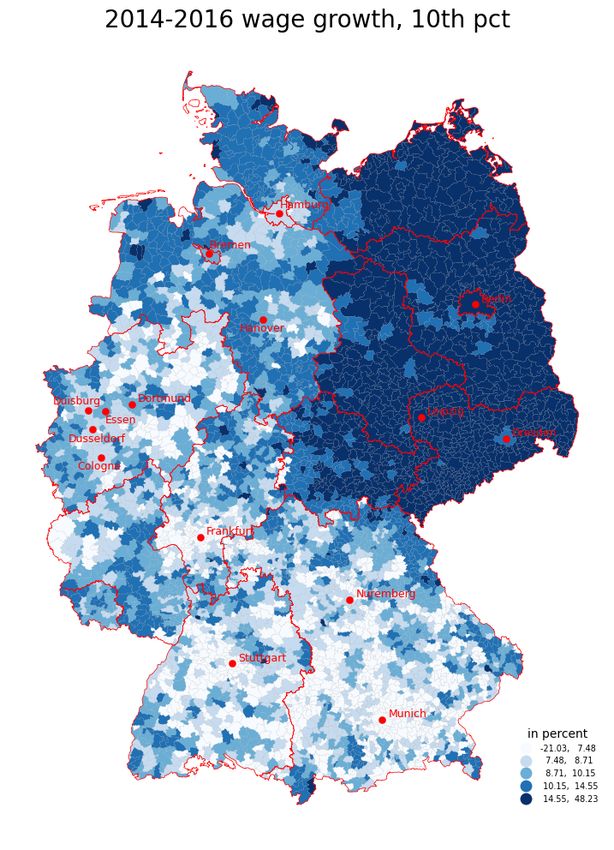
minimum wage (54% of the national median wage)1 as of 2015 provides an opportunity to
contrast theoretical predictions with evidence. Second, we are able to quantify the model
at unprecedented spatial coverage and detail at the level of 4,421 micro regions (Verbands-
gemeinden), owing to the availability of linked linked-employer-employee data covering
the universe of 30M workers from the Institute for Employment Research (IAB) and a
micro-geographic property price index recently developed by Ahlfeldt et al. (2021). Third,
our ability to observe the spatial economy in the recent past before a minimum wage was
introduced greatly simplifies the quantification since we can treat observed labour market
outcomes as undistorted market outcomes.
    This data set paves the way for our methodological contribution, which is to develop
a quantitative spatial model with heterogeneous firms that possess monopsony power. We
start from a canonical setup in the spirit of Redding and Rossi-Hansberg (2017). Workers
choose where to live, where to work and how much to consume of a composite tradable
good and housing, trading expected wages and amenities against commuting cost, goods
prices and housing rents. Goods are produced in a monopolistically competitive market
and traded at a cost. Housing is supplied inelastically, creating a congestion force that
restores the spatial equilibrium. We extend this canonical framework in three important
respects. First, we borrow from the trade literature and introduce a Pareto-shaped pro-
ductivity distribution of firms (Redding, 2011; Gaubert, 2018). This extension is critical
to generating a wage distribution within regions and enabling the minimum wage to real-
locate workers to more productive establishments. Second, we follow Egger et al. (2021),
who build on Card et al. (2018), and generate an upward-sloping labour supply curve to
the firm via Gumbel-distributed idiosyncratic preferences for employers, in addition to al-
lowing for idiosyncrasy in preferences for residence and workplace locations (Ahlfeldt et al.,
2015).2 This extension is critical to awarding employers monopsony power. Third, we gen-
erate imperfectly elastic aggregate labour supply via a Gumbel-distributed idiosyncratic
utility from non-employment. This extension is critical to capturing incentives minimum
wages can create for workers to become active on the labour market and search for jobs
(Mincer, 1976; Lavecchia, 2020).
    To develop the intuition for the regional employment response in our model, it is in-
structive to consider three firm types. The minimum wage has no effect on the most
productive firms, which we term unconstrained because they voluntarily pay wages above
the minimum wage. These firms still exercise their full monopsony power after the min-
imum wage is introduced. For all less productive firms, the minimum wage is binding.
These firms can no longer lower the wage below the minimum wage, which implies that
they lose some of their monopsony power. The more productive among the constrained
firms will respond by hiring all workers they can attract at the minimum wage—the new
   1
      This quantity is based on the hourly wages of full-time and part-time workers (see Section 2.2 for
further information). Based on the wages of full-time workers, the Minimum Wage Commission reports
that the Kaitz Index was 46% in Germany in the year 2018 (Mindestlohnkommission, 2018)
    2
      Dustmann et al. (2021) model non-pecuniary aspects of job choice in a similar way.

                                                   2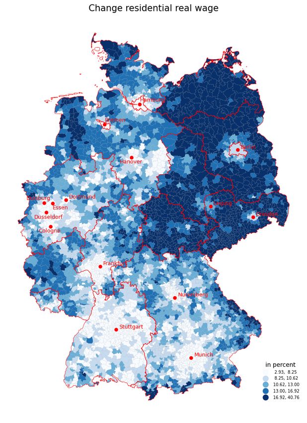
marginal cost of labour—which is why we refer to them as supply-constrained. Consequen-
tially, they will increase employment. Less productive firms will hire until the marginal
revenue product falls below the minimum wage level, which is why we term them demand-
constrained. While some demand-constrained firms will react to the introduction of the
minimum wage by increasing employment, any demand-constrained firm that produces at
a MRPL below the minimum wage will have to reduce employment to stay in the mar-
ket once a minimum wage is introduced. The aggregation of the employment response
across all firms within a region delivers the prediction that the regional employment ef-
fect of a federal minimum wage is a hump-shaped function of regional productivity. We
substantiate this predictions in two complementary approaches.
   In the first step, we employ a reduced-form methodology that uses high-productivity
regions in which firms are mostly unconstrained as a counterfactual in the spirit of a dy-
namic difference-in-difference model. This approach allows us to test a central prediction
of the model without imposing the full structure of the quantitative model. Consistent
with model predictions, we find that the employment response is flat in the regional wage
level for high-productivity regions, where the 2014 mean hourly wage exceeds e18.6. Com-
pared to this group, regions with a mean hourly wage of more than e13.1 tend to gain
employment whereas those with a lower mean wage tend to lose. These estimates of
a theory-consistent regional distribution of minimum-wage induced employment effects
adds to a literature that has mostly focused on average effects for selected spatial units
(e.g. Card and Krueger, 1994; Dustmann et al., 2021) or point estimates of the effect of
the minimum wage bite (e.g. Machin et al., 2003; Ahlfeldt et al., 2018). Indirectly, they
provide evidence supporting the monopsonistic labour market model that is still scarce
(Neumark, 2018). Importantly, we bring to light a sizable negative employment effect in
the least productive micro regions that has gone unnoticed in previous studies analyzing
larger spatial units (Ahlfeldt et al., 2018; Caliendo et al., 2018; Dustmann et al., 2021).
   In the second step, we quantify the full model to take the analysis into the general
equilibrium. We exploit our matched worker-establishment micro data to estimate the
structural parameters that govern the wage distribution within regions. We then invert
the model in 2014—the year before the introduction of the minimum wage. Solving the
model under the minimum wage of 48% of the national mean that we observe in our
data delivers the comparative statics from which we infer the minimum wage effect. We
find almost exactly the same regional wage levels that characterize the hump-shape of the
regional employment response as in the reduced-form analysis. The important advantage
of the model-based general-equilibrium approach is that we do not have to assume any
group of firms, workers, or regions to be unaffected by the minimum wage, which allows
us to establish the aggregate employment effect. While the hump-shape in the model
resembles our reduced-form estimates, we gain the additional insight that employment
increases in regions of intermediate productivity at the expense of the least and most
productive regions. In the national aggregate, employment decreases by about 0.3% or
100K jobs, which is less than predicted by the competitive labour market model (Knabe

                                             3
et al., 2014).
   For our purposes, the ability of our model to speak to welfare effects is, at least, as im-
portant as establishing aggregate employment effects. We find that the German minimum
wage has increased welfare by 2%. This estimate of the minimum wage welfare effect is
unprecedented in the literature in that it accounts for changes in nominal wages, employ-
ment probabilities, goods prices, housing rents, the quality of the worker-firm match, the
reallocation of workers across firms, commuting destinations, residences, and the growing
number of workers who decide to be active on the labour market. In other words, the
increase in real wage—adjusted for changes in tradeble goods prices, housing rents, and
commuting costs—dominates the reduction in the employment probability. As as a result,
about 180K workers become active on the labour market and start searching for jobs.
Again, there is significant spatial heterogeneity. The net-winners are low-productivity re-
gions such as in the eastern states, resulting in long-run incentives for workers to relocate
to regions that have experienced sustained population loss over the past decades.
   Given the absence of a credible counterfactual, we cannot over-identify the aggregate
effects of the German minimum wage our model delivers. We show, however, that the
model’s predictions for minimum wage effect in wages, employment, housing rents and
commuting distances are closely correlated with observed before-after changes in the data
at the regional level. We also show that our model predicts changes in the Gini coeffi-
cient of wage inequality across all workers in all regions that are in line with before-after
changes observed in data. This suggests significant out-of-sample predictive power, which
is reassuring with respect to our key normative contribution: The derivation of optimal
minimum wage schedules.
   To this end, we compute aggregate employment and welfare effects for a broad range
of federal and regional minimum-wage schedules. We also provide an equity measure
based on the Gini coefficient of wage inequality. Hence, we equip our readers with the
key ingredients to compute their own optimal minimum wage. Under canonical welfare
functions, the optimal federal minimum wage will not be lower than the employment-
maximizing minimum wage, at 38% of the national mean wage. Up to 60%, the minimum
wage can be justified on the grounds of welfare effects. Higher levels require equity (among
those in employment) as an objective. Ambitious minimum wages need to be defended
against negative employment effects that start building up rapidly beyond 50% of the
national wage. Against this background, it is important to note that the employment-
maximizing regional minimum wage, at 50% of the regional mean wage, would deliver
positive welfare effects that are similar to the federal welfare-maximizing minimum wage
(4%), plus increase employment by 1.1%, suggesting that regional minimum wages are
targeted policy instruments that warrant more attention.
   With these results, we contribute to the identification of turning points where the costs
of minimum wages start exceeding the benefits, a challenge that allegedly lies ahead of the
field (Manning, 2021). In doing so, we complement a large literature using reduced-form
approaches that suggest that minimum wages may (Meer and West, 2016; Clemens and

                                              4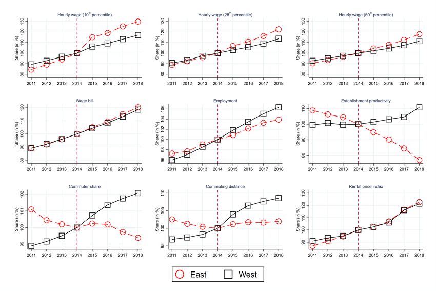
Wither, 2019) or may not have negative employment effects (Dube et al., 2010; Cengiz
et al., 2019).3 This includes a growing literature evaluating the labour market effects of
the German minimum wage, which we review in more detail in Appendix A (e.g. Ahlfeldt
et al., 2018; Bossler and Gerner, 2019; Caliendo et al., 2018; Dustmann et al., 2021).
We also contribute to a smaller normative literature on minimum wages that considers
distributional effects of minimum wages (Lee and Saez, 2021; Simon and Wilson, 2021).4
For Germany, Drechsel-Grau (2021) studies the macroeconomic and distributional effects
of minimum wages within a dynamic macroeconomic model in a current working paper.
    Our theoretical contribution builds on a literature showing that, in a monopsonis-
tic labour market,5 a minimum wage can raise the wage without reducing employment
(Stigler, 1946; Manning, 2003a).6 We also draw from a literature on quantitative spatial
models, which have recently emerged as general-purpose tools for policy evaluation that
can account for mobility of residents across residence and workplace locations (Allen and
Arkolakis, 2014; Ahlfeldt et al., 2015).7 In particular, our model nests Monte et al. (2018)
as a special case in which the dispersion of firm productivity approaches infinity, there is
no idiosyncrasy in worker tastes for employers, and workers supply labour inelastically.
    Most closely, we connect to a small literature that studies the effects of minimum wages
in a spatial equilibrium. Our contribution complements Monras (2019) and Simon and
Wilson (2021) who consider a competitive labour market. To our knowledge, the only
other model that nests a monopsonistic labour market in a spatial general equilibrium is
in the current working paper by Bamford (2021), who also provides an evaluation of the
German minimum wage. Similar to us, he uses worker-firm-specific idiosyncratic utility
to generate an upward-sloping labour-supply curve to the firm. By making the labour
supply elasticity dependent on the density of nearby firms within relatively large regions
that roughly correspond to local labour markets, he shows that lower monopsony power
acts as an important concentration force in the spatial economy (see also Azar et al.
(2019)). In contrast, our focus is the development of a comprehensive welfare measure
for the normative evaluation of minimum wages. Hence, we develop our model at the
micro-regional level to capture minimum wage effects on commuting costs explicitly.8 We
also account for how frictional trade shapes the spatial distribution of minimum wage
effects and account for employment and welfare effects that arise when minimum wages
incentivize workers to become active on the labour market, which is important to enable
     3
       A new wave of empirical minimum wage research, based on difference-in-differences designs, started
with the seminal paper by Card and Krueger (1994) whose findings, subsequently challenged by Neumark
and Wascher (2000), cast doubt on the competitive labour market model which predicts that binding
minimum wages necessarily lead to job loss.
     4
       Minimum wages also interact with the optimal tax system (Allen, 1987; Guesnerie and Roberts, 1987).
     5
       Manning (2020) offers a recent review of the literature.
     6
       Similarly, search models do not restrict the sign of the employment effect of a minimum wage (Brown
et al., 2014; Blömer et al., 2018).
     7
       Other recent models that quantitatively account for commuting include Tsivanidis (2019); Heblich et
al. (2020); Almagro and Domínguez-Iino (2021).
     8
       We generate larger employment elasticities (Monte et al., 2018) and less monopsony power in thicker
labour markets as workers can substitute across commuting destinations (Manning, 2003b; Datta, 2021).

                                                    5
aggregate employment gains.
   The remainder of the paper is structured as follows. Section 2 introduces the insti-
tutional context and our data, and presents stylized evidence that informs our modelling
choices. Section 3 introduces a partial equilibrium version of our model and provides
transparent reduced-form evidence that is consistent with stylized predictions. Section
4 develops the full quantitative model and takes the analysis to the general equilibrium.
Section 5 concludes.

2 Empirical context
In this section, we introduce the German minimum wage policy, the various sources of
data we rely on, and some stylized facts that inform our modelling choices.

2.1 The German minimum wage
The first uniformly binding federal minimum wage in Germany was introduced in 2015.
Since then, German employers had to pay at least e8.50 euros per hour corresponding to
48% of the mean salary of full-time workers. Because no similar regulation preceded the
statutory wage floor, it represented a potentially significant shock to regions in the left
tail of the regional wage distribution. Subsequently, the minimum wage has been raised to
e8.84 in 2017, e9.19 in 2019 and e9.35 in 2020. In relative terms, it has fluctuated within
a close range of 47% to 49% of the national mean wage, suggesting that it is reasonable
to treat the introduction of the minimum wage as a singular intervention in 2015. We
provide a detailed discussion of the institutional context in Section 2.1.

2.2 Data
We compile a novel data set for German micro regions that is unique in terms of its
national coverage of labour and housing market outcomes at sub-city level. We provide a
brief summary of the various data sources here and refer to Appendix B.2 for details.

Employment, establishments and wages. We use the Employment Histories (BeH)
and the Integrated Employment Biographies (IEB) provided by the Institute for Em-
ployment Research (IAB) which contain individual-level panel data containing workplace,
residence, establishment, wage, and characteristics such as age, gender, and skill on the
universe of about 30M labour market participants in Germany.

Hours worked. We follow Ahlfeldt et al. (2018) and impute average working hours
separately for full-time and part-time workers from an auxiliary regression that accounts
for the sector of employment, federal state of employment, and various socio-demographic
attributes and using the 1% sample from the 2012 census. We find that full-time employees
work approximately 40 hours per week while the number is lower for regularly employed
(21 hours) and for marginally employed part-time workers (10 hours). Combining working
hours with average daily earnings delivers hourly wages.

                                             6
Real estate. We use a locally-weighted regression approach proposed by Ahlfeldt et
al. (2021) to generate an area-year housing cost index. The raw data comes from Im-
moscout24, accessed via the FDZ-Ruhr (Boelmann and Schaffner, 2019). It covers nearly
20 million residential observations between 2007 and 2018.
Trade. Trade volumes are taken from the Forecast of Nationwide Transport Relations in
Germany which are provided by the Clearing House of Transport Data at the Institute of
Transport Research of German Aerospace Center. The data set contains information about
bilateral trade volumes between German counties in the year 2010 for different product
groups. Following Henkel et al. (2021), we aggregate trade volumes across all modes of
transport (road, rail and water). To convert volumes (measured in metric tonnes) into
monetary quantities, we use information on national unit prices for the different product
groups. Finally, we aggregate the value of trade flows across all product groups.
Spatial unit. The primary spatial unit of analysis are 4,421 municipal associations (Ver-
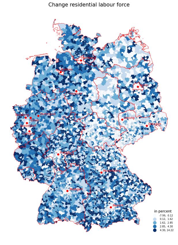
bandsgemeinden) according to the delineation from 31 December 2018 (see Figure 1 for a
map). Municipal associations are spatial aggregates of 11,089 municipalities (Gemeinden)
that ensure a more even distribution of population and geographic size. Henceforth, we
refer to municipal associations as municipalities for simplicity. On average, a municipal-
ity hosts 541 establishments employing 6,769 workers on less than 80 square kilometers,
making it about a tenth of the size of an average county. For each pair of municipalities,
we compute the Euclidean distance using the geographic centroids.
2.3 Stylized facts
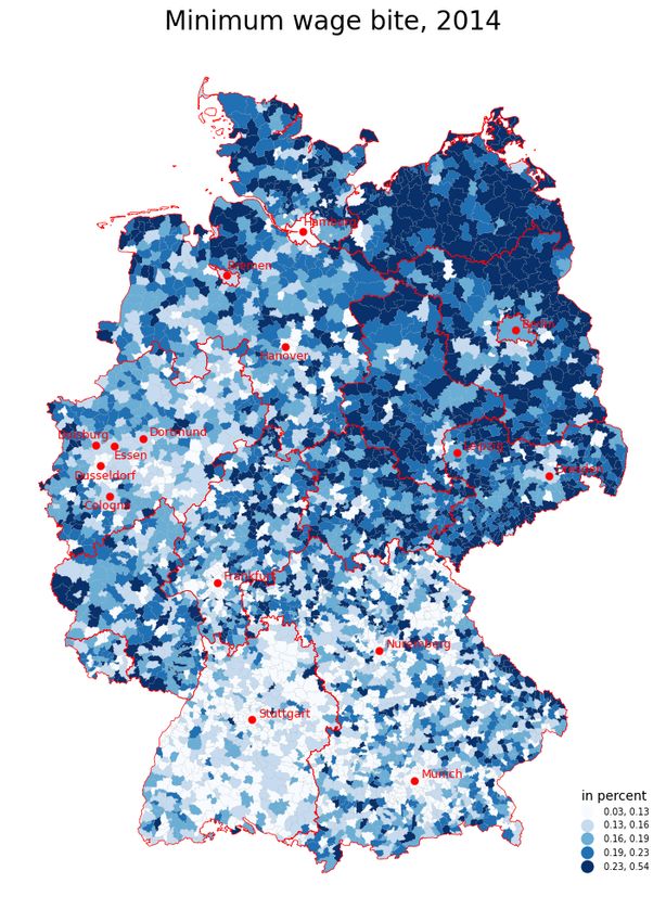
Figure 1, illustrates a measure of the regionally differentiated “bite” of the national min-
imum wage, very much in the tradition of Machin et al. (2003). Concretely, we compute
a bite exposure measure at the residence by taking the average over the shares of below-
minimum-wage workers at the workplace across nearby municipalities, weighted by the
bilateral commuting flows in 2014.9 This way, we capture the bite within the actual com-
muting zone of a municipality. Evidently, the minimum wage had a greater bite in the
east, in line with the generally lower productivity. Changes in low wages, defined as the
10th percentile in the within-area wage distribution, from 2014 to 2016 closely follow the
distribution of the bite, suggesting a significant degree of compliance. Together, the two
maps suggest that the minimum wage contributed to the reduction of spatial wage dispar-
ities in Germany, an impression that we substantiate with further evidence in Appendix
B.3.
The striking heterogeneity in the policy-induced wage increase between the eastern and
the western states makes it instructive to compare how employment and other outcomes
evolved in the respective parts of the country over time. We offer this purely descriptive
9 ∑ L
Formally, we define the bite as Bi = j
∑ i,j SjM W , where Li,j is the number of employees who live
j Li,j
in municipality i and commute into municipality j for work and SjM W is the share of workers compensated
below the minimum wage in j.
7
Figure 1: Minimum wage bite and change in 10th pct. regional wages

       (a) Minimum wage bite in 2014                              (b) 2014-2016 wage growth at 10th pct.

Note: Unit of observation is 4,421 municipality groups. The 10th percentile wage refers to the 10th percentile in
the distribution of individuals within a workplace municipality, re-weighted to the residence using commuting flows.
Wage and employment data based on the universe of full-time workers from the BeH.

comparison in Figure 2. Confirming Figure 1, a jump at the 10th percentile of the wage
distribution in the east is immediately apparent. A more moderate increase is also visible
for the west. For higher percentiles, it is possible to eyeball some increase in the east, but
not in the west. A first-order question from a policy-perspective is whether the policy-
induced wage increase came at the cost of job loss as predicted by the competitive labour
market model. While we argue that—without a general equilibrium model—it is difficult
to establish a counterfactual for aggregate employment trends, the absence of an imme-
diately apparent employment effect in these time series is still informative. It is worth
noticing that, while employment continues to grow in both parts of the country after the
minimum wage introduction, the rate of growth appears to slow down in the east compared
to the west. However, even if one is willing to interpret this as suggestive evidence of a
negative employment effect, it will be difficult to argue that negative employment effects
turned out to be as severe as in some pessimistic scenarios circulated ahead of the imple-
mentation (Ragnitz and Thum, 2008). Since, following the minimum-wage introduction,
the aggregate wage bill increases in the east, relative to the west, it seems fair to conclude

                                                         8
Figure 2: Outcome trends in western and eastern states
Note: All time series are normalized to 100% in 2014, the year before the minimum wage introduction. The
establishment wage premium is the employment-weighted average across firm-year fixed effects from a decomposition
of wages into worker and firm fixed effects following Abowd et al. (1999) (see Appendix B.4 for details).
that a positive wage effect has dominated a possibly negative employment effect, pointing
to positive welfare effects. Figure 2 also illustrates the reallocation of workers to more
productive establishments at greater commuting distance documented by Dustmann et al.
(2021). Indeed, it appears that the effect has gained momentum subsequent to 2016, when
their analysis ends. Finally, there appears to be a slight increase in the rate of property
price appreciation after the minimum wage which could be reflective of increased demand.
These stylized facts echo a growing empirical literature on the effects of the German
minimum wage which we summarize in Appendix A. They motivate us to develop a quan-
titative spatial model that nests a monopsonistic labour market in which a statutory
minimum wage triggers different employment responses by firms of distinct productivity
and workers decide where to live and work trading higher wages against greater commuting
costs.
3 Partial equilibrium analysis
In this section, we develop a model of optimal behaviour of heterogeneous firms in a
monopsonistic labour market with a minimum wage. We first use the model to develop the
intuition for why the employment response to a uniform minimum wage differs qualitatively
9across firms, depending on their productivity. We then derive the novel prediction that the
regional employment response is a hump-shaped function of regional productivity. Finally,
we provide novel area-specific estimates of the employment effect of the minimum-wage
that confirm this prediction.
3.1 Model I
For now, we take upward-sloping labour supply to the firm as well as downward-sloping
product demand as exogenously given. We nest the firm problem introduced here into
a QSM in Section 4. The extended model will provide the micro-foundations for the
labour supply and product demand functions and allow us to solve for the spatial general
equilibrium of labour, goods, and housing markets.
3.1.1 Optimal firm behaviour
A firm in location j ∈ J sells its product variety at monopolistically competitive goods
markets across all locations i ∈ J. Because one firm produces only one variety, we use ωj
to denote both a firm and its variety. Given a productivity φj , firm ωj hires lj (ωj ) units of
labour in a monopsonistically competitive labour market which it uses to produce output
yj (ωj ) = φj (ωj )lj (ωj ).
Labour supply. Firm ωj faces an iso-elastic labour supply function
hj (ωj ) = Sjh [ψj (ωj )wj (ωj )]ε (1)
of the expected wage ψj (ωj )wj (ωj ) that a worker earns in this firm, with wj (ωj ) > 0 being
the firm’s wage rate and ψj (ωj ) ∈ (0, 1] being the firm’s hiring probability. Unless otherwise
indicated, we assume ψj (ωj ) = 1 to ease notations. We denote the firm’s constant labour
supply elasticity by ε > 0 and introduce Sjh > 0 as an aggregate shift variable that
summarizes all general equilibrium effects operating through location j’s labour market
(specified in more detail below and solved in general equilibrium in Section 4).
Goods demand. Similarly, there is iso-elastic demand for variety ωj in location i
qij (ωj ) = Siq pij (ωj )−σ , (2)
which depends inversely on the variety’s consumer price pij (ωj ) with a constant price
elasticity of demand σ > 1, and which is directly proportional to an aggregate shift
variable Siq > 0 that summarizes all general equilibrium effects operating through location
i’s goods market (specified in more detail below and solved in general equilibrium in
Section 4). Under profit maximization and goods market clearing, we can express the
revenue function as
X 1
rj (ωj ) = pij (ωj )qij (ωj ) = Sjr σ
[yj (ωj )]ρ , (3)
i
10P 1−σ q
where ρ = σ−1
σ ∈ (0, 1). Intuitively, a greater market access Sjr ≡ i τij Si > 0 implies
that a smaller fraction of output melts away due to iceberg trade costs τij ≥ 1, leading to
relatively larger revenues (see Appendix C.1).
Minimum wage. In deriving the effects of a statutory minimum wage w on price,
output, and labour input, it is instructive to distinguish between three firm-types: uncon-
strained firms (indexed by superscript u), for which the minimum wage w is non-binding;
supply-constrained firms (indexed by superscript s), whose labour demand exceeds labour
supply at the binding minimum wage w; and demand-constrained firms (indexed by su-
perscript d), that attract more workers than they require when the minimum wage w is
binding. We present the key results for the three firm types below and refer to Appendix
C.2 for further derivations. As each firm can be fully characterized by its productivity level
and its firm-type, we drop the firm index ωj in favour of a more parsimonious notation,
combining the firm’s productivity level φj with superscript z ∈ {u, s, d}.
Unconstrained firms choose profit-maximizing wages that are larger or equal to the
minimum wage level. Therefore, we can use the labour supply function to the firm in Eq.
(1) to derive the relevant cost function
− 1 ε+1
ε u
cuj (φj ) = wju (φj )lju (φj ) = Sjh lj (φj ) ε . (4)
Facing an upward-sloping labour supply function, firms can only increase their employment
by offering higher wages. Hence, the average cost of labour ACL(φj ) = cuj (φj )/lju (φj )
is upward-sloping as illustrated in Figure 3. The marginal cost of labour M CL(φj ) =
ε+1
∂cuj (φj )/∂lju (φj ) = ε ACL(φj ) is also upward-sloping and strictly greater than ACL(φj ).
Since demand for any variety is downward-sloping, an expansion of production and labour
input is associated with a lower marginal revenue product of labour M RP L(φj ) = ∂rju (φj )/∂lju (φj ).
Unconstrained firms find the profit-maximizing employment level by setting M RP L(φj ) =
M CL(φj ) which corresponds to point a in Figure 3. Since a higher productivity shifts
the M RP L(φj ) function outwards, more productive firms hire more workers at higher
wages (Oi and Idson, 1999). Unconstrained firms simultaneously act as monopolists in the
goods market and monopsonists in the labour market, setting their prices as a constant
mark-up σ/(σ − 1) > 1 over marginal revenues and their wages as a constant mark-
down ε/(ε + 1) < 1 below marginal costs. The combined mark-up/mark-down factor is
1/η ≡ [σ/(σ − 1)][(ε + 1)/ε] > 1.
We refer to φuj as the least-productive unconstrained firm that is identified by setting
wj (φuj ) = w, so we obtain
σ ! 1
u 1 σ−1 Sjh σ−1
σ+ε
φj (w) = w σ−1 . (5)
η Sjr
All firms with φj < φuj are constrained by the minimum wage. Any increase in the
minimum wage level will lead to a firm with a greater productivity becoming the marginal
11Figure 3: Optimal firm employment
wjz (φj )
M CL(φj ) ACL(φj )
b a
M RP L(φuj )
c b
w b b
M RP L(φsj )
ljz (φj )
lju (φuj )
unconstrained firm.
Supply-constrained firms face a binding minimum wage, resulting in M RP L(φj ) = w.
At this wage, workers are willing to supply no more than hsj (φj ) = Sjh wε units of labour,
which corresponds to lju (φuj ) in Figure 3. Employment is constrained by labour supply
because supply-constrained firms would be willing to hire more workers as the MRPL
function intersects with w at an employment level greater than lju (φuj ). In the absence
of the minimum wage, supply-constrained firms would set a wage below w to equate
MRPL and MCL. At this wage, workers would supply less than lju (φuj ) units of labour.
By removing the monopsony power, the mandatory wage floor raises employment for all
firms with φsj ≤ φj < φuj , where φsj defines the least-productive supply-constrained firm
given by
σ
η σ−1 u η ε
φsj (w) = φj (w) < φuj (w) with = < 1. (6)
ρ ρ ε+1
Notice that all supply-constrained firms set the same wage (i.e. the minimum wage) and
hire the same number of workers ljs (φj ) = hs (φj ) = wε Sjh = lju (φuj ), (determined by b in
Figure 3).
Demand-constrained firms also face a binding minimum wage, resulting in M RP L(φj ) =
w. For these firms with productivities φj < φsj (w), however, employment is constrained
by labour demand because at a wage of w firms demand less units of labour than workers
are willing to supply. To see this, consider the MRPL curve for any firm with produc-
tivity φj < φsj in Figure 3, which will be below M RP L(φsj ). Since w intersects with
the MRPL before it intersects with ACL, there is job rationing with a hiring probability
12ψjd (φj ) = ljd (φj )/hdj (φj ) < 1. Yet, demand-constrained firms do not necessarily reduce em-
ployment. As long as a demand-constrained firm is sufficiently productive for its MRPL
curve to be above point c, the MRPL in the monopsony market equilibrium exceeds w.
Therefore, the intersection of MRPL and w is necessarily to the right of the intersection of
MRPL and MCL, implying greater employment under the minimum wage. The opposite
is true, however, for any firm whose productivity is sufficiently small for the MRPL curve
to be below point c. Because the MRPL in the monopsony market equilibrium is smaller
than w, the firm has to reduce output and labour input to raise the MRPL to the minimum
wage level.
3.1.2 Aggregate outcomes
Having characterized the optimal behaviour of the three firm types, we now explore how the
introduction of a minimum wage affects aggregate outcomes at the regional level. To this
end, we assume that firm productivity follows a Pareto distribution with shape parameter
k > 0 and lower bound φj > 0. For the following discussion, it is instructive to introduce
the critical minimum wage levels wzj ∀ z ∈ {s, u} as a function of φj . They are implicitly
defined through φzj (wzj ) = φj ∀ z ∈ {s, u} and have the following interpretation: For a
sufficiently small minimum wage, w < wuj , location j features only unconstrained firms.
For higher minimum wages, w < wsj , location j also features supply-constrained, but no
demand-constrained firms. Using Eq. (5), we obtain
! 1
Sjr σ+ε
wuj = wju (φj ) = η σ φσ−1 (7)
j Sjh
as an implicit solution to φuj (wuj ) = φj . Using Eq. (5) in Eq. (6) and solving φsj (wsj ) = φj
for wsj results in
! 1
Sr
σ−1 j
σ+ε
wsj = ρσ φj , (8)
Sjh
σ
implying wsj /wuj = (ρ/η) σ+ε > 1. Using these critical minimum wages we derive the
following proposition:
Proposition 1. Assuming Pareto-distributed firm productivities, aggregate employment
Lj , aggregate labour supply Hj and aggregate revenues Rj are hump-shaped in the minimum
wage level. Aggregate profits, Πj , are declining in w.
Proof see Appendix C.4.
To develop the intuition, let’s first consider the region indexed by j = 1 in panel a)
of Figure 4. Any minimum wage w1 ≤ wu1 will have no effect because all firms in the
region are unconstrained as they voluntarily set higher wages. A marginal increase in
w1 turns some unconstrained firms into supply-constrained firms, whose response to the
loss of monopsony power is to hire all workers who are willing to supply their labour at
wage wu1 . Hence, regional employment increases. Once w1 > ws1 , some firms become
13Figure 4: Regional employment, minimum wages and productivity
Lj (w, φj ) ∆Lj (w, φj )
b
b b
b b
0
b b
1
L1 (w, φ1 ) L2 (w, φ2 )
w φj
wu1 wu2 = wmax
1 wmax
2 φmin φ′j φj
′′
φ′′′
j
j
(a) Minimum wages (b) Regional productivity
Note: In this partial-equilibrium illustration, we assume constant general equilibrium terms {Sjr , Sjh } that are
invariant across regions and not affected by the minimum wage.
demand-constrained. The marginal effect of an increase in w1 remains initially positive
even beyond ws1 because demand-constrained firms still increase the labour input as long
as their MRPL exceeds w1 in the monopsony market equilibrium. At some point, however,
w1 will exceed the MRPL of the least productive firms in the market equilibrium and these
firms will respond by reducing output and labour input. The marginal effect of w1 declines
and becomes zero at the employment-maximizing minimum wage wmax
1 . Further increases
have negative marginal effects and, eventually, the absolute employment effect will turn
negative. The generalizable insight is that for given fundamentals {Sjr , Sjh } and regional
productivity summarized by φj , aggregate employment Lj (wj , φj ) is hump-shaped in the
minimum wage level wj .
To clear the regional labour market, the hump-shaped pattern must carry through to
labour supply. Since the hiring probability is ψjz = 1 ∀ z ∈ {s, u} for unconstrained and
supply-constrained firms, labour supply defined in Eq. (1) increases for low but binding
minimum wage levels wuj ≤ wj < wsj . At a higher minimum wage level, the expected
hiring probability adjusts to the hiring rate to account for the job rationing of demand-
constrained firms (ψjd (φj ) = ljd (φj )/hdj (φj )). In other words, workers who are unlikely to
get a job withdraw from the labour force. In the spatial general equilibrium introduced
in Section 4.1, workers will adjust labour supply by choosing if to work and where to live
(migration) and work (commuting). For a discussion of the effect of the minimum wage
on firm profits and revenues, we refer to Appendix C.4.
Let us now compare the effect of a uniform minimum wage in region j = 1 to a
region j = 2 in which firms are generally more productive, for example, due to better
infrastructure or institutions. To ease the comparison, we normalize initial employment to
14unity. A low minimum wage wu1 < w ≤ wmax
1 leads demand- and supply-constrained firms
to hire more workers in region j = 1, whereas there is no employment effect in region j = 2
since all firms remain unconstrained. At a higher level wmax
1 < w < wmax
2 , an increase
in the minimum wage reduces employment in region j = 1 because the MRPL of the
marginal firm falls below w, whereas employment increases in region i = 2 owing to the
loss of monopsony power of formerly unconstrained firms. Hence, the same increase in the
minimum wage level can have qualitatively different employment effects in different regions
because the employment-maximizing minimum wage depends on regional productivity.
This is an important theoretical result that rationalizes why a large empirical literature
has failed to reach consensus regarding the employment effects of minimum wage rises
(Manning, 2021).
Of course, regional productivity not only affects the marginal effect of a minimum wage
increase, but also the aggregate effect relative to the situation without a minimum wage.
In panel (a) of Figure 4, the aggregate effect is given by ∆Lj (w, φj ) = Lj (wj ) − Lj (wuj ).
In panel (b) of Figure 4, we plot ∆Lj (w, φj ) against φj , which directly maps into the
average regional productivity given the Pareto-shaped firm productivity distribution. We
consider a continuum of regions with heterogeneous productivity, but only one universal
national minimum wage w, which resembles the empirical setting in Germany and many
other countries. We refer to Appendix C.5 for a detailed and formal discussion of the
comparative statics. Briefly summarized, we can distinguish between three types of re-
gions. The minimum wage has no effect in regions where even the least productive firm
′′′
is unconstrained (φj ≥ φj ). In the least productive regions, there are negative aggregate
′
employment effects driven by demand-constrained firms (φj < φj ). In between, there
are positive employment effects driven by supply-constrained firms (and some demand-
′′
constrained firms) that peak at the regional productivity level φj . Hence, the regional
employment effect of a national minimum wage is hump-shaped in regional productiv-
ity. This is a novel theoretical prediction which we take to the data using a transparent
reduced-form methodology before we return to the model to establish the spatial general
equilibrium.
3.2 Reduced-form evidence
To empirically evaluate the central prediction that the regional employment effect of the
German national minimum wage is hump-shaped in regional productivity, we require es-
timates of the minimum wage effect by spatial units that are sufficiently small to exhibit
sizable variation in average productivity. The empirical challenge in establishing the re-
gional minimum wage effect is that the counterfactual outcome in the absence of the min-
imum wage is unlikely to be independent of the regional productivity level φj . Consider
the following data generating process (DGP):
h i
ln Lj,t = f + f (φj ) I(t ≥ J ) + aj + tbj + ϵj,t , (9)
15where J = 2015 is the year of the minimum wage introduction, Lj,t is employment in area
j in year t, aj is a 1 × J vector of regional fixed effects and bj is a vector of parameters
that moderate regional-specific time trends of the same dimension. aj is likely positively
correlated with employment since more productive regions attract more workers. Condi-
tional on aj , bj can be positively or negatively correlated with employment depending
on whether the economy experiences spatial convergence or divergence. ϵj,t is a random
error term. Unless we hold aj and tbj constant, we will fail to recover the correct con-
ditional expectation E[ln Lj,t |φj ), t ≥ J ] − E[ln Lj,t |φj ), t < J ]. To address this concern,
we difference Eq. (9) twice to get
[ln Lj,t − ln Lj,t−n ] − [ln Lj,t−n − ln Lj,t−m ] = ∆2 ln Lj = f + f (φj ) + ϵ̃i,t , (10)
where t − n < J , t − m < J and ϵ̃i,t is the twice differenced error term. Guided by the
theoretical predictions summarized in Figure 4, we define the relative (up to the constant
f ) before-after minimum wage effect as a polynomial spline function
f (φj ) = E ∆2 ln Lj |wjmean , (wmeanj ≤ α0 ) − E ∆2 ln Lj |wjmean , (wmeanj > α0 )
X2
(11)
= 1 wjmean ≤ α0 × αg wjmean − α0 ,
g
g=1
with the theory-consistent parameter restrictions {α0 > α1
2α2 , α1 < 0, α2 < 0}. Since
higher fundamental productivity maps to higher wages in our model, we use the 2014
mean wage wjmean as a proxy for regional productivity. Notice that the interpretation of
f (φj ) is akin to the treatment effect in an intensive-margin difference-in-difference setting
in which regions populated solely by unconstrained firms form a control group to establish
a counterfactual.
Substituting in Eq. (11), we are ready to estimate Eq. (10) for given years {t, t − n, t −
m}. To obtain parameter values {α0 , α1 , α2 }, we nest an OLS estimation of {α1 , α2 } in
a grid search over a parameter space α0 ∈ [αo , ᾱo ] and pick the parameter combination
that minimizes the sum of squared residuals. From the identified parameters {α0 , α1 , α2 },
there is a one-to-one mapping to regional mean wage levels that correspond to regional
′ ′′ ′′′
productivity levels {φj , φj , φj } in Figure 4 (see Appendix C.6 for details). Note that
consistent with the partial-equilibrium nature of the analysis, Eq. (11) lends a difference-
in-difference interpretation to the predicted employment effect fˆ(φ ) as regions dominated
j
′′′
by unconstrained firms (φj ≥ φj }) serve as the counterfactual.
In the DGP laid out in Eq. (9), we assume that the linear area-specific trends extend
from the [t − m, t − n] to the [t − n, t] period. This assumption is more likely to be true
over shorter study periods. Hence, we set {t = 2016, m = 4, n = 2} in Figure 5, which
restricts the comparison to two years before and after the minimum wage introduction.
The results with one- or three-year windows are very similar (see Appendix C.6).
Consistent with theory, we find an employment effect that is hump-shaped in the 2014
16Figure 5: Regional minimum wage effects: Reduced-form evidence
.01
Employment effect of minimum wage (∆ln(L))
-.09 -.07 -.05
-.11 -.03 -.01
Rel. min. wage = 64% Rel. min. wage = 53% Rel. min. wage = 46%
9 10 11 12 13 14 15 16 17 18 19 20 21
2014 area mean wage (EUR)
Note: Dependent variable is the second difference in log employment over the 2012-14 and 2014-16 periods. Markers
give averages within one-euro bins, with the marker size representing the number of municipalities within a bin.
The last bin (22) includes all municipalities with higher wages because observations are sparse. The red solid line
illustrates the quadratic fit, weighted by bin size. Two outlier bins are excluded to improve readability, but they
are included in the estimation of the quadratic fit. Confidence bands (gray-shaded area) are at the 95% level. The
relative minimum wage is the ratio of the 2015 minimum wage level w = 8.50 over the 2014 mean wage (when there
was no minimum wage).
mean wage. The greatest positive employment effect is predicted for an area with a 2014
′′
mean wage of about e16, which corresponds to φj . The implication is that the regional
employment effect is maximized for the area where the relative minimum wage amounts
to e8.5/e16=53% of the mean wage. Municipalities with a lower mean wage, where
the relative minimum wage is higher, have smaller predicted employment effects. At a
relative minimum wage of 64% the predicted employment effect turns negative, a point
′
that corresponds to φj in Figure 4. The empirical correspondent to productivity level
′′′
φj —beyond which the minimum wage has no bite— is a regional mean wage of e18.6,
which corresponds to a relative minimum wage of 46%.
The 46-64% range for the relative minimum wage derived in this section represents a
first point of reference for those wishing to ground the minimum-wage setting in trans-
parent reduced-form evidence of employment effects. Yet, the reduced-form approach
constrains us to identifying relative employment effects. By assumption, we do not cap-
ture any general equilibrium effects that affect the control group (unconstrained regions).
Moreover, the reduced-form approach naturally does not allow us to derive the welfare
effect, which not only depends on the effects on wages and employment probabilities, but
also on changes in commuting costs, tradable goods and housing prices. We, therefore,
take the analysis to the spatial general equilibrium in the next section.
174 General equilibrium analysis
We develop the model in Section 4.1 and discuss the quantification in Section 4.2 before
lay out how to use the model for quantitative counterfactual analyses in Section 4.3.
Then, we proceed to a three-step application. First, we use the model to quantitatively
evaluate the general equilibrium effects of the German minimum wage introduced in 2015
in a counterfactual analysis in Section 4.4.1. Second, we treat the model’s predictions of
changes in endogenous outcomes as forecasts that we subject to over-identification tests
by comparing them to observed before-after changes in the data in Section 4.4.2. Third,
we find the optimal minimum wage in a series of counterfactuals in which we consider a
range of national and regional minimum wages in Section 4.5.
4.1 Model II
Building on the partial equilibrium framework introduced in Section 3.1, we now expand
the model to account for the interaction of goods and factor markets, free entry of firms
and an endogenous choice of workers to enter the labour market. We refer to N̄ as the
working-age population and denote the labour force measured at the place of residence i
by Ni and the labour force measured at the workplace j by Hj . Lj represents employment
(at the workplace) and can generally be smaller than the labour force when minimum
wages are binding.
4.1.1 Preferences and endowments
Workers are geographically mobile and have heterogeneous preferences to work for firms in
different locations. Given the choices of other firms and workers, each worker maximizes
utility by choosing a residence location i and a (potential) employer φj – thereby pinning
down the (potential) workplace location j. The preferences of a worker ν who lives and
consumes in location i and works at firm φj in location j are defined over final goods
consumption Qiν , residential land use Tiν , an idiosyncratic amenity shock exp[bijν (φj )],
and commuting costs κij > 1, according to the Cobb-Douglas form
α 1−α
exp[bijν (φj )] Qiν Tiν
Uijν (φj ) = . (12)
κij α 1−α
The amenity shock captures the idea that workers can have idiosyncratic reasons for living
in different locations and working in different firms (Egger et al., 2021). We assume that
bijν (φj ) is drawn from an independent Type I extreme value (Gumbel) distribution
Fij (b) = exp(−Bij exp{−[εb + Γ′ (1)]}), with Bij > 0 and ε > 0, (13)
in which Bij is the scale parameter determining the average amenities from living in
location i and working in location j, ε is the shape parameter controlling the dispersion of
amenities, and Γ′ (1) is the Euler-Mascheroni constant (Jha and Rodriguez-Lopez, 2021).
18The goods consumption index Qi in location i is a constant elasticity of substitution
(CES) function of a continuum of tradable varieties
σ
XZ
σ−1
Qi = dφj
σ−1
qij (φj ) σ (14)
j φj
with qij (φj ) > 0 denoting the quantity of variety φj sourced from location j and σ > 1 as
the constant elasticity of substitution. Utility maximization yields qij (φj ) = Siq pij (φj )−σ
σ−1
with Siq ≡ EiQ PiQ as defined in Eq. (2), in which EiQ is aggregate expenditure in
location i for tradables, PiQ is the price index dual to Qi in Eq. (14), and pij (φj ) is the
consumer price of variety φj in location i.
The economy is further endowed with a fixed housing stock T̄i . Denoting by EiT total
expenditure for housing in location i, we can equate supply with demand, TiD = EiT /PiT ,
to derive the market-clearing price for housing:
T
T Ei
Pi = . (15)
T̄i
4.1.2 Free entry and goods trade
Firms learn their productivity φj only after paying market entry costs, fje PjT , which consist
of some start-up space fje acquired at housing rent PjT . The investment is profitable
whenever expected profits exceed these costs and we refer to this relation as the free-entry
condition given by
Πj
π̃j = = fje PjT . (16)
Mj
Using the facts that Πj = (1 − η)[ΦΠ R
j (w)/Φj (w)]Rj and that also the aggregate wage bill
is proportional to revenues, w̃j Lj = [1 − (1 − η)ΦΠ R
j (w)/Φj (w)]Rj , we can reformulate Eq.
(16) to get
j (w)(1 − η)
ΦΠ w̃j Lj
Mj = , (17)
ΦR
j (w) − ΦΠ (w)(1 − η) P T f e
j j j
where
Rj − Πj 1 − (1 − η)ΦΠ R R
j (w)/Φj (w) χR Φj (w) u
w̃j = = wj (φj ) (18)
Lj η χL Φ L
j (w)
denotes the average wage rate in location j which is proportional to the cut-off wage wju (φj )
of an unconstrained firm with productivity φj given that wju (φj )lju (φj )/η = rju (φj ) =
πju (φj )/(1 − η).
With firm entry costs being paid in terms of housing and assuming that land owners
spend their entire income on the tradable good, we can state that total housing expenditure
in location i is given by EiT = (1 − α)ṽi Ni + Πi and aggregate expenditure on tradable
goods results as
EiQ = αṽi Ni + EiT = ṽi Ni + Πi , (19)
19where ṽi is the average labour income of the residential labour force Ni across employment
locations.
Building on optimal firm behaviour derived in Section 3.1, our model implies a gravity
equation for bilateral trade between locations. Using the CES expenditure function and the
measure of firms Mj , the share of location i’s expenditure on goods produced in location
j is given by
R
Mj pij (φj )1−σ dG(φj )
φj
θij = P R ,
1−σ dG(φ )
k∈J Mk φk pik (φk ) k
n o 1−σ (20)
Mj ΦPj (w) ΦL (w)/[Φ R (w) − (1 − η)ΦΠ (w)] τ w̃ /φ
j j j ij j j
=P 1−σ .
M Φ P (w) Φ L (w)/[ΦR (w) − (1 − η)ΦΠ (w)] τ w̃ /φ
k∈J k k k k k ik k k
R
To derive Eq. (20) we take advantage of the ideal price index Pij ≡ [ φj pij (φj )1−σ dφj ]1/(1−σ)
for the subset of commodities that are consumed in location i and produced in location j.
As formally shown in Appendix C, it can be computed as
1 1 1
Pij = χP1−σ ΦPj (w) 1−σ Mj1−σ puij (φj ), (21)
with χP > 1 as a constant and ΦPj (w) > 0 as a term that captures the aggregate effect
of the minimum wage w on the price index Pij . Notice that ΦPj (w) = 1 if the minimum
wage w is not binding in location j. If the minimum wage is binding, Φpj (w) can be
larger or smaller than one, reflecting two opposing forces: Supply-constrained firms and
highly productive demand-constrained firms lose their monopsony power and therefore
set lower prices, which reduces the average price of firms from location j. At the same
time, a binding minimum wage raises the costs – in particular for unproductive demand-
constrained firms, which pass through this increase to their consumers in form of higher
prices. The expenditure share θij declines in bilateral trade costs τij in the numerator
(“bilateral resistance”) relative to the trade costs to all possible sources of supply in the
denominator (“multilateral resistance”).
Using optimal prices together with Eqs. (18) and (21) to substitute for Pij , puij (φj ),
P
and wju (φj ), into the price index (PiQ )1−σ ≡ j Pij1−σ dual to the consumption index in
Eq. (14) we obtain
" #1−σ 1−σ
1
X ΦL
j (w)
1
χL τij w̃j
PiQ = χ 1−σ
Mj ΦPj (w) ,
χR P Φj (w) − (1 − η)Φj (w) φj
R Π
j (22)
1−σ
1
χL 1−σ1
Mi ΦPi (w) ΦL
i (w) τii w̃i
= χP ,
χR θii ΦR
i (w) − (1 − η)ΦΠ
i (w) φi
which we can rewrite in terms of location i’s own expenditure share θii .
Location j’s aggregate labour income w̃j Lj is proportional to aggregate revenue Rj in
20You can also read