Optimal Power Flow in Deregulated Power Systems by Using Optimization Techniques
←
→
Page content transcription
If your browser does not render page correctly, please read the page content below
Optimal Power Flow in Deregulated Power Systems by Using Optimization
                                  Techniques

      M.Sindhu1; G.V. Nagesh Kumar2; Vempalle Rafi3*; B. Sravan Kumar4; M. Aruna Bharathi5
     1
          PG Student, Department of Electrical and Electronics Engineering, JNTUA College of Engineering
                                             Pulivendula, Kadapa, India.
 2
   Professor, Department of Electrical and Electronics Engineering, JNTUA College of Engineering Pulivendula,
                                                    Kadapa, India.
3*
   Assistant Professor (A), Department of Electrical and Electronics Engineering, JNTUA College of Engineering
                                             Pulivendula, Kadapa, India.
                                             3*
                                               vempallerafi@gmail.com
           4
            Assistant Professor, Department of Electrical and Electronics Engineering, GITAM University,
                                                Vishakhapatnam, India.
     5
       Professor, Department of Electrical and Electronics Engineering, Geethanjali College of Engineering and
                                            Technology, Hyderabad, India.

 Abstract
 An independent system operator tasked with providing equitable and fair transmission services in an
 open-market context has a challenging job in dynamic security-constrained dispatch of an electric
 power network. This study proposes a new methodology based on the optimal flow of power and
 swarming mode, which is restricted by iterative stability. In addition to the static and dynamic
 functional constraints, dynamic margin needs in relation to normal condition and contingencies,
 particle swarm and moth swarm optimizations are used to optimize social welfare. Furthermore,
 because the pattern of load growth in the current market environment is difficult to forecast, a new
 approach for estimating the sensitive loading direction linked with a dynamic loading margin is
 presented. To demonstrate and test the suggested approach, an IEEE 14-bus test system with both
 supply and demand bids is utilized.

 Key-words: Current Market Environment, Load Growth, Particle Swarm Optimization, Moth Swarm
 Algorithm.

 1. Introduction

         The functioning of the power system has been meticulously studied with the deregulation of
 the power flow process. With ever-increasing demand, the majority of industrialized countries are

ISSN: 2237-0722                                                                                          1883
Vol. 11 No. 3 (2021)
Received: 02.01.2021 – Accepted: 18.05.2021
constructing new transmission lines. System operators who provide market players with sufficient,
realistic methods for evaluating, maintaining, and pricing system security in order to consider
transactions in a secure market. However, load demand rose as a result of the requirement to operate
the power system, including economic concerns, resulting in several considerations surrounding the
power system's operation and security.
Charges include stability, safety and dependable grid electricity operation in an autonomous
system with distinct environmental operators (ISOs). Complex simulations and models are included
through suitable system pricing with security limitations and diverse concerns. The different models,
including security [1, 2], were proposed on the market.
The likelihood of bifurcation relies on the loading level of the system. In severely loaded
systems, the attraction region is relatively tiny as the operating point approaches the maximum load
point on the P-V curve [5], which makes the system unable to withstand any disturbances. For HB,
the analysis includes the detection and prediction of bifurcation sites close to power systems. The
index fork is a common approach. It's one way.
The prediction is suggested [6–8] utilizing HB and SNB indices. A novel method for
identification for bifurcation includes the load rising step variable. For detection in accordance with
the index in [9] of the Dynamic Loading Margin (DLM) method and with load-increasing steps. This
technique of bifurcation detection detects the event in five or six iterations. In addition, in system
management it is important to determine the sensitive load direction of the network. Comprehensive
study has been carried out into the calculation of the loadability margin, given the stability of static
voltage [10–14].
Continuous flow can be the most accurate approach for calculating the load-bearing margins
in a particular charge direction by tracing system curves P-V that can be linked to an SNB or LB [10,
11]. In [12], a maths method for calculating an SNB closet and a worst case load capacity buffer for
collapse of voltage was described. The worst loading direction for SNB is obtained by this approach.
In [13] the maximum loading condition was estimated by the iterative and direct power flow method.
In [14] the authors suggested a modified continuation flow for stationary comportment of power
system tracking owing to variations in parameters. This method has a continuation method for
tracking the solution curve using a predictor corrector. In static models all of the above strategies
consider SNB alone.
The paper offers a sensitive direction of the load with an iterative load, including SSC-OPF. A
novel method for the analysis of the SSC-OPF sensitive load direction. The PSO method involves
optimisation. It is used. The suggested approach, which incorporates the security margin function
ISSN: 2237-0722 1884
Vol. 11 No. 3 (2021)
Received: 02.01.2021 – Accepted: 18.05.2021solution in accordance with the contingency criterion N-1. Maximize social welfare goals which
cover and maintain the adequate distance with voltage parameters at bus or system stability limits, to
the maximum loading situation.
2. Normal OPF- Market
The market for OPF-hinged optimization, a restricted nonlinear issue, comprises optimization
with an objective function that contains a set of equality and inequality constraints, as illustrated
below:
Min. f ( x, p, k ),
s.t. g ( x, p) = 0,
hmin h( x, p, k ) hmax (1)
p min p p max
The f, g, and h functions were considered with the objective function including as
f ( x, p, k ) = −(C DT Pd − C ST PS ). ( 2)
The negative producer surplus, in addition to the consumer surplus, is represented by Eq. (2),
i.e., the social net benefit.
Equality constraints: The flow of power is represented by g(x, p) =0 using conventional
formulae.
g ( x, p, k ) = g ( , V , QG , PS , Pd ) = 0. (3)
The usual steady-state depiction of system loads includes constant PQ loads with constant
power factor that are supposed to increase for the purpose of stressing the system as follows:
PL = PL 0 + Pd ,
Pd kPL 0 , (4)
Q L = PL tan ,
PG = PGo + PS .
Inequality constraints: Inequality limits are the system's physical and security restrictions.
Transmission line thermal limitations were addressed in the physical and security limits.
I ij ( ,V ) I ij max . (5)
Generator Reactive power limits:
QG min QG ( ,V ) QG max . (6)
ISSN: 2237-0722 1885
Vol. 11 No. 3 (2021)
Received: 02.01.2021 – Accepted: 18.05.2021Voltage “Security” limits:
Vmin V Vmax (7)
Power limits on Transmission lines:
Pij ( ,V ) Pij max . (8)
Which are used to represent the security limits of the system.
The limits are represented as follows:
Ps min Ps Ps max ,
(9)
Pd min Pd Pd max .
3. OPF with Small Perturbation Stability Constraints
a. Modelling
To analyze accurately in order to bifurcate for a particular system, including the use of correct
dynamical models. In order to assess tiny signal stability in power networks, load flow and dynamical
equations are required. With the speed of the equation, the dynamic state varies and
increases/decreases. Dynamic order, on the other hand, is diminishing, which may result in low
accuracy.
b. Determination of Bifurcation
The bifurcation occurrence in power system of Eigen values in state matrix depends on its
position with the pair of Eigen values, which reaches the imaginary axis with non-zero imaginary part
of complex term when HB occurs.
The DLM is considered in power system with different loadings and the range of output varies
between initial and final position of loading directions for estimating the dynamic stability states of
the system for power flow in the buses.
To determine the distance the simplest way in the system is bifurcation point method, which
includes and depend on three stages. Different stages include by increasing load, by decreasing load,
by varying load either increasing or decreasing within the limits for the optimization in the power
system. There are many iterations in the bifurcation method for power flow study.
ISSN: 2237-0722 1886
Vol. 11 No. 3 (2021)
Received: 02.01.2021 – Accepted: 18.05.2021c. Market-clearing Model SSC-OPF
The following optimization model is used to describe an OPF market clearing model with
minor perturbation stability requirements in this article: it is a non-linear optimization problem with
an implicit constraint that is solved using an optimization approach. The PSO approach is utilized as
the foundation to solve the given optimization issue in this study.
d. Sensitivity Analysis for Load Direction
This article represents an OPF marketing clearance model, with the inclusion of modest
stability restrictions, with the following optimization issue: non-linear optimization fundamentally
with an implied restriction; this problem is addressed by a technique of optimization. The PSO
approach is utilized as the foundation to solve the given optimization issue in this study.
Overview of PSO
Multi-agent search technology is PSO which follows the progress of a birds' flock in the
emerging movement in the quest for food. It employs a variety of swarming particles. In a PSO
system, particles fly into a multifaceted search area. During the flight, each particle changes its
location through its own neighbouring particle experiences and uses the best place its neighbours find
themselves in. Each particle passes through the search space to find the smallest world (or
maximum). With the historical experience of a set of its surrounding particles and of itself, the swarm
direction of a particle is determined.
Each particle’s new velocity and position is given in equations. (10) and (11):
pvd +1 = cf *[ * pvd + ac1rand() * ( pbest − ppd ) + ac2rand () * (Gbest − ppd )] , (10)
ppd +1 = ppd + pvd +1 (11)
Here, rand() is a uniform random value lies between [0,1], and cf is the constraint factor given
as Eq. (12):
2
cf = , (12)
2 − ac − ac2 − 4ac
Where ac=ac1+ac2 and ac≥4.
The resolution will be defined by areas between the current location and the target position to
be looked for. This restriction improves local problem space exploration. The progressive changes of
ISSN: 2237-0722 1887
Vol. 11 No. 3 (2021)
Received: 02.01.2021 – Accepted: 18.05.2021human learning are likewise simulated realistically. When PVmax is excessively large, it is possible
that particles overlook suitable solutions.
However, a modest PVmax prevents particles from exploring local solutions adequately. Lastly,
the PSO can be reduced to local minimum. PVmax was frequently set at 10–20% of the dynamic range
of the variable on every dimension in numerous encounters with PSO [27]. The declining weight of
the inertia in [28, 29] is presented and tested for global search at the beginning of the algorithm,
followed by local searches. If the weight of inertia is not lowered with time, a value 2 is advised.
Numerous parameters deemed acceptable for some of the common functions in many research
suggest different values [29].
The simulating process is generally utilized for optimization issues, including equality (13)
and inequality restrictions with the fitness function:
Min. f ( x),
s.t. g ( x) = 0, (13)
h h( x ) h
Where x is vector of variables optimisation i.e. with limits. 'f’ is the function for scalar
optimisation; ‘g’ is the vector equality function given in Eq. (3); and ‘h’ is a vector inequality with ‘h’
limits (lower and upper). The calculated process is PSO, with the following stages.
Step 1. Input system specifications that define the bounds of each variable and constraint.
Step 2. For each Pv, the particles must be randomly started with population from a random
uniform distribution in the interval.
pv max = ( pp max − pp min ) * . (14)
The Pbest initial individual set consists of I initial locations of is individual, and Gbest is the
initial position found with the least amount of fitness.
Step 3. Eq.(10) is used to update the velocity vector. The parameters in Equations (10) and
(12) are chosen as follows:
γ=0.7968, ac1=ac2=2. (15)
Step 4. Considering the position limitations to change: each position is altered by Eq.(11)
depending on their current speed. If the individual element of a certain element exceeds its
restrictions and has to be replaced by n particles which meet its limitations.
Step 5. Pbest and Gbest updates; the Pbest of every particle is updated as follows throughout the
system:
ISSN: 2237-0722 1888
Vol. 11 No. 3 (2021)
Received: 02.01.2021 – Accepted: 18.05.2021d +1
Pbest i
= ppid +1 if Fi d +1 Fi d ,
d +1
(16)
Pbest i
= ppid if Fi d +1 > Fi d .
The fitness function is Fi and is defined in Eq (2). for individual i. Gbest in dC1 is a collection
of the best locations among Pbest elements that has been assessed.
Step 6.end iterations must be used as a stop condition and repeated steps shall be fulfilled
through step 3. The operation is halted if the maximum number of iterations is reached.
4. Mixed Sensitive Loading Direction SSC-OPF
The technology proposed for SSC-OPF with a sensitive loading direction linked with an ideal
market solution is shown in Figure 1. Flowchart If the DLM method for calculating and detecting the
sensitive load direction is completed for each particle, the time required to execute this operation is
too costly for any bigger system. The sensitive direction of the related DLM is calculated after SSC-
OPF is executed in the suggested technique.
The following is the technique:
• In the first iteration, the initial generation and load specify the increased load direction of
the DLM computation. The loading parameter, the basis case or pure market clearing
problem, will be initialized.
• The maximum loading level for the operating point can be set to k in this situation. SSC-
OPF is solved with the current parameter value as outlined in Eq. (17).
Min. f ( x, p, k ) = −(C DT Pd − C ST PS ),
s.t. g ( ,V , QG , PS , Pd , k ) = 0,
k = kˆ, (17)
hmin h( x, p, k ) hmax ,
p min p pmax ,
• The present SSC-OPF load-enhancing N solution, utilized for estimation of sensitive
loading direction, in the starting direction.
• Ni means the direction of loading with the DLM method which, by considering the SSC-
OPF solution with its beginning value, operating circumstances and sensible direction,
determines the DLM. The direction of load increases is taken into account.
• Definition of sensitive direction following SSC-OPF, either with or without DLMreq,
related with the DLM sensitive direction.
ISSN: 2237-0722 1889
Vol. 11 No. 3 (2021)
Received: 02.01.2021 – Accepted: 18.05.2021• If the process is stopped by DLM > DLMreq, the procedure will then resume to step 1 by
utilizing the DLM for SSC-op calculation with the sensible loading with direction acquired
in step 2. Note that contingencies may be considered directly to allow for effective handling
of system security. Furthermore, this repeated procedure allows the value of the loading
parameters to be controlled.
Fig. 1 - Flow Chart of Proposed SSC-OPF-SLD
Numerical Results
If the process is stopped by DLM > DLM req, the procedure will then resume to step 1 by
utilizing the DLM for SSC-op calculation with the sensible loading with direction acquired in step 2.
Note that contingencies may be considered directly to allow for effective handling of system security.
Furthermore, this repeated procedure allows the value of the loading parameters to be controlled.
Table 1 shows the market bidding data (the GENCO and ESCO numbers in this table correspond to
ISSN: 2237-0722 1890
Vol. 11 No. 3 (2021)
Received: 02.01.2021 – Accepted: 18.05.2021the bus number in Figure 2). This system has the capacity to mimic a market in power, producing
relevant results that enable analyzing the strategies suggested.
Fig. 2 - Single Line Diagram of the IEEE 14 Bus System
The advantage of method proposed in power system with the DLM, which includes input and
output data sets. N – 1 contingency are used in DLM detection and estimation method. The PSO
method for optimization is used for optimality which includes and abolishes the Lagrangian with
complexity and computation of multi-player.
PSO convergence, including step by step algorithms in Figure 5. PSO convergence. The study
comprises a collection of 30 particles. In [16], the number of particles improved from 30 to 50 leads
to quicker convergence. In the range of 0.3 and 0.4, the load sensitivity with the DLM needed is
shown in Figure 6. The suggested approach for identifying the sensitive load direction converges in
around seven iterations. When the DLM with the OPF operating point is needed when the output
changes, different direction of load is necessary.
Moth Swarm Algorithm (MSA)
A novel algorithm of high standard, inspired by moth orientation to moonlight. Two new
operators were suggested for optimization:
ISSN: 2237-0722 1891
Vol. 11 No. 3 (2021)
Received: 02.01.2021 – Accepted: 18.05.20211. Dynamic crossover approach for the management of vectors of difference based on
population diversity Lévy-mutation improves exploration capacity in the recognition phase.
2. Immediate memory associated learning process. Simulate a moth short-term memory,
decrease the memory required and overcome the classical-initial PSO's speed issue. In the
celestial navigation stage this technology is utilized for small-scale operation.
5. Simulation Results
a) PSO Algorithm
Evaluating for the K-Factor: 0.05
PSO: 1/20 iterations, GBest = 0.040601
PSO: 20/20 iterations, GBest = 0.034799
Voltage values at buses are:
Columns 1 through 7: 1.0043 1.0027 1.0042 1.0007 1.0073 1.0066 1.0027
Columns 8 through 14: 1.0026 1.0040 1.0096 1.0050 1.0074 1.0082 1.0098
Power values at buses are:
Columns 1 through 7: 2.5035 0.4051 0 0.0372 0.1435 1.0017 0.0808
Columns 8 through 14: 0.2307 0.1191 0.5083 0.1584 0.0648 0.0957 0.3136
Social Welfare = 26.2075 dollars
Evaluating for the K-Factor: 0.1
PSO: 1/20 iterations, GBest = 0.081207
PSO: 20/20 iterations, GBest = 0.069603
Voltage values at buses are:
Columns 1 through 7: 1.0038 1.0050 1.0061 1.0000 1.0068 1.0036 1.0009
Columns 8 through 14: 1.0002 1.0030 1.0094 1.0015 1.0029 1.0055 1.0077
ISSN: 2237-0722 1892
Vol. 11 No. 3 (2021)
Received: 02.01.2021 – Accepted: 18.05.2021Power values at buses are:
Columns 1 through 7: 2.6519 0.4051 0 0.0390 0.1504 1.0494 0.0847
Columns 8 through 14: 0.2417 0.1248 0.5325 0.1660 0.0680 0.1003 0.3286
SocialWelfare = 57.1332 dollars
Evaluating for the K-Factor: 0.15
PSO: 1/20 iterations, GBest = 0.1218
PSO: 20/20 iterations, GBest = 0.1044
Voltage values at buses are:
Columns 1 through 7: 1.0070 1.0070 1.0011 1.0036 1.0085 1.0096 1.0077
Columns 8 through 14: 1.0078 1.0068 1.0032 1.0042 1.0026 1.0005 1.0055
Power values at buses are:
Columns 1 through 7: 2.7904 0.4051 0 0.0407 0.1572 1.0971 0.0885
Columns 8 through 14: 0.2527 0.1304 0.5567 0.1735 0.0710 0.1048 0.3435
SocialWelfare = 88.1811 dollars
Evaluating for the K-Factor: 0.2
PSO: 1/20 iterations, GBest = 0.1624
PSO: 20/20 iterations, GBest = 0.1392
Voltage values at buses are:
Columns 1 through 7: 1.0087 1.0094 1.0046 1.0098 1.0036 1.0003 1.0059
Columns 8 through 14: 1.0017 1.0097 1.0010 1.0096 1.0017 1.0048 1.0016
Power values at buses are:
Columns 1 through 7: 2.8351 0.4051 0.0993 0.0425 0.1641 1.1448 0.0924
Columns 8 through 14: 0.2637 0.1361 0.5809 0.1811 0.0741 0.1094 0.3585
SocialWelfare = 114.4853 dollars
ISSN: 2237-0722 1893
Vol. 11 No. 3 (2021)
Received: 02.01.2021 – Accepted: 18.05.2021Evaluating for the K-Factor: 0.25
PSO: 1/20 iterations, GBest = 0.203
PSO: 20/20 iterations, GBest = 0.17399
Voltage values at buses are:
Columns 1 through 7: 1.0086 1.0034 1.0061 1.0005 1.0051 1.0043 1.0064
Columns 8 through 14: 1.0027 1.0092 1.0088 1.0033 1.0038 1.0099 1.0098
Power values at buses are:
Columns 1 through 7: 2.8790 0.4051 0.1912 0.0443 0.1708 1.1925 0.0962
Columns 8 through 14: 0.2747 0.1418 0.6051 0.1886 0.0772 0.1139 0.3734
SocialWelfare = 141.3997 dollars
Evaluating for the K-Factor: 0.3
PSO: 1/20 iterations, GBest = 0.2436
PSO: 20/20 iterations, GBest = 0.20879
Voltage values at buses are:
Columns 1 through 7: 1.0087 1.0002 1.0008 1.0018 1.0036 1.0095 1.0022
Columns 8 through 14: 1.0060 1.0057 1.0049 1.0064 1.0025 1.0030 1.0030
Power values at buses are:
Columns 1 through 7: 2.9224 0.4051 0.2834 0.0461 0.1777 1.2402 0.1001
Columns 8 through 14: 0.2857 0.1475 0.6293 0.1962 0.0803 0.1185 0.3884
SocialWelfare = 168.7674 dollars
Evaluating for the K-Factor: 0.35
PSO: 1/20 iterations, GBest = 0.28419
PSO: 20/20 iterations, GBest = 0.24359
Voltage values at buses are:
Columns 1 through 7: 1.0087 1.0074 1.0046 1.0076 1.0085 1.0085 1.0026
ISSN: 2237-0722 1894
Vol. 11 No. 3 (2021)
Received: 02.01.2021 – Accepted: 18.05.2021Columns 8 through 14: 1.0061 1.0034 1.0045 1.0098 1.0098 1.0057 1.0018
Power values at buses are:
Columns 1 through 7: 2.9649 0.4051 0.3763 0.0478 0.1845 1.2879 0.1039
Columns 8 through 14: 0.2967 0.1531 0.6534 0.2037 0.0833 0.1229 0.4033
SocialWelfare = 196.6277 dollars
----WHEN lINE 1-5 OUTAGE HAPPENS ----
Evaluating for the K-Factor: 0.15
PSO: 1/20 iterations, GBest = 0.12181
PSO: 20/20 iterations, GBest = 0.1044
Social Welfare value = 0.00000 dollars
DLM value= 0.34992 dollars
Evaluating for the K-Factor: 0.2
PSO: 1/20 iterations, GBest = 0.16242
PSO: 20/20 iterations, GBest = 0.13921
Social Welfare value = 23.86645 dollars
DLM value = 0.33374 dollars
Evaluating for the K-Factor: 0.25
PSO: 1/20 iterations, GBest = 0.20301
PSO: 20/20 iterations, GBest = 0.174
Social Welfare value = 48.00707 dollars
DLM value = 0.31869 dollars
Evaluating for the K-Factor: 0.3
PSO: 1/20 iterations, GBest = 0.24363
PSO: 20/20 iterations, GBest = 0.20881
Social Welfare value = 69.77609 dollars
DLM value = 0.26386 dollars
ISSN: 2237-0722 1895
Vol. 11 No. 3 (2021)
Received: 02.01.2021 – Accepted: 18.05.2021Evaluating for the K-Factor: 0.35
PSO: 1/20 iterations, GBest = 0.28419
PSO: 20/20 iterations, GBest = 0.24359
Social Welfare value = 91.96020 dollars
DLM value = 0.23164 dollars
The sensitive load direction for SSC-OPF (SLD) -----------------------
Evaluating for the DLM : 0.3
PSO: 1/20 iterations, GBest = 0.28421
PSO: 20/20 iterations, GBest = 0.2436
Power values at buses are:
Columns 1 through 7: 2.2199 0.9094 0.4136 0.0445 0.1777 1.2402 0.1002
Columns 8 through 14: 0.2854 0.1309 0.6293 0.1962 0.0803 0.1185 0.3884
Social Welfare value = 151.24479 dollars
Evaluating for the DLM: 0.4
PSO: 1/20 iterations, GBest = 0.28421
PSO: 20/20 iterations, GBest = 0.2436
Power values at buses are:
Columns 1 through 7: 1.8498 1.0127 0.5007 0.0401 0.1777 1.2402 0.0770
Columns 8 through 14: 0.2857 0.1134 0.5248 0.1932 0.0803 0.1185 0.3884
Social Welfare value = 116.80279 dollars
---WHEN lINE 1-5 OUTAGE HAPPENS -----
Evaluating for the DLM : 0.3
PSO: 1/20 iterations, GBest = 0.28423
PSO: 20/20 iterations, GBest = 0.24362
Power values at buses are:
Columns 1 through 7: 1.9445 1.0127 0.6076 0.0461 0.1777 1.2402 0.0818
Columns 8 through 14: 0.2857 0.1322 0.6228 0.1962 0.0803 0.1185 0.3884
ISSN: 2237-0722 1896
Vol. 11 No. 3 (2021)
Received: 02.01.2021 – Accepted: 18.05.2021Social Welfare value = 64.12333 dollars
Evaluating for the DLM: 0.4
PSO: 1/20 iterations, GBest = 0.28424
PSO: 20/20 iterations, GBest = 0.24362
Power values at buses are:
Columns 1 through 7: 1.7026 1.0127 0.6076 0.0354 0.1777 1.2402 0.0982
Columns 8 through 14: 0.2857 0.1134 0.4841 0.1960 0.0803 0.1185 0.3354
Social Welfare value = 36.82892 dollars
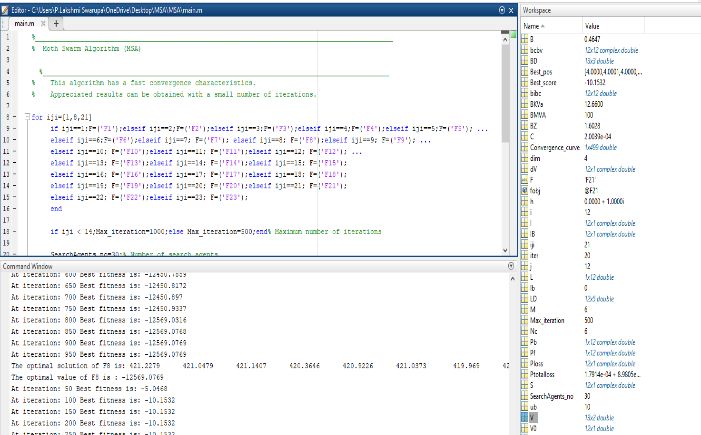
b) Moth Swarm Algorithm (MSA):
Fig. 3 - MSA Algorithm in MATLAB
ISSN: 2237-0722 1897
Vol. 11 No. 3 (2021)
Received: 02.01.2021 – Accepted: 18.05.2021Fig. 4 - Simulation of MSA in Command Prompt
Fig. 5 - Fitness Value Versus No. of Iterations
ISSN: 2237-0722 1898
Vol. 11 No. 3 (2021)
Received: 02.01.2021 – Accepted: 18.05.2021Fig. 6 - Fitness Value Versus No. of Iterations 1000/1000
Fig. 7 - Fitness Value Versus No. of Iterations 500/500
MSA: 1/500 iterations, GBest = 0.26324
MSA: 500/500 iterations, GBest = 0.23362
Power values at buses are:
ISSN: 2237-0722 1899
Vol. 11 No. 3 (2021)
Received: 02.01.2021 – Accepted: 18.05.2021Columns 1 through 7: 1.6014 1.1011 0.7021 0.0321 0.1657 1.2201 0.0912
Columns 8 through 14: 0.1834 0.1134 0.3713 0.1673 0.0513 0.1081 0.3251
Social Welfare value = 10.1532 dollars
6. Analysis
The Moth Swarm Algorithm (MSA) is a novel method for meta-heuristic optimisation
inspired on moth navigation. This work provides a new modified MSA with an arithmetic crossover
(MSA-AC) to enhance the global search for the best solution, the speed of convergence and the
performance of a classical MSA.
7. Conclusion
This study proposes a strategy based on the iterative SSC-OPF-SLD that incorporates a
stability constraint together with the sensitive direction of loading into the energy system. The
sensitive direction of loading is based on normal vector calculation. The results show the advantages
of the technology suggested to give an ideal solution for the market, depending on system safety and
the innovative Moth Swarm Algorithm (MSA) which is inspired by moth direction towards
moonlight, in order to tackle limited optimal power flow (OPF) problems. In addition to adaptive
Gaussian walks and spiral motion, the associational mechanism for the development of instantaneous
memory and population diversity crossover for Lévy-mutation has been suggested. The MSA
technique therefore enables system operators to study the influence of system safety on the process of
market clearance. In addition, the PSO approach is used to optimize this issue. Compared to several
previous studies OPF methods based on PSO, the efficacy and superiority of MSA has been shown to
be straightforward to implement and to discover optimal solutions to the non-linear, restricted issue.
References
Milano, F., Canizares, C.A., and Invernizzi, M., “Multi-objective optimization for pricing system
security in electricity markets,” IEEE Trans. Power Syst., Vol. 18, No. 2 pp. 596–604, May 2003.
Milano, F., Canizares, C.A., and Conejo, A.J., “Sensitivity-based security-constrained OPF market
clearing model,” IEEE Trans. Power Syst., Vol. 20, No. 4, pp. 2051–2060, November 2005.
Marszalek, W., and Trzaska, Z. W., “Singularity-induced bifurcations in electrical power systems,”
IEEE Trans. Power Syst., Vol. 20, No. 1, pp 312–320, February 2005.
ISSN: 2237-0722 1900
Vol. 11 No. 3 (2021)
Received: 02.01.2021 – Accepted: 18.05.2021Yue, M., Brookhaven National Lab, “Bifurcation subsystem and its application in power system analysis,” IEEE Trans. Power Syst., Vol. 19, No. 4, pp. 1885–1893, 2004. Canizares, C.A., “On bifurcation voltage collapse and load modeling,” IEEE Trans. Power Syst., Vol. 10, No. 1, pp. 512–522, February 1995. Canizares, C.A., Mithulananthan, N., Milano, F., and Reeve, J., “Linear performance indexes to predict oscillatory stability problems in power system,” IEEE Trans. Power Syst., Vol. 19, No. 2, pp. 1023–1031, May 2004. Tomim, M.A., Lopes, B.I.L., Leme, R.C., Jovita, R., Zambroni de Souza, A. C., de Carvalho Mendes, P. P., and Lima, J. W. M., “Modified Hopf bifurcation index for power system stability assessment,” IEE Proc. Generat. Transm. Distrib., Vol. 152, No. 6, pp. 906–912, November 2005. Hasanpor Divshali, P., Hosseinian, S.H., Nasr Azadani, E., and Vahidi, B., “Modified fast indices for prediction of Hopf bifurcation by matrix reciprocal condition number,” The Iranian Conference on Electrical Engineering (ICEE 2008), Tehran, Iran, May 2008. Wen, X., A Novel Approach for Identification and Tracing of Oscillatory Stability and Damping Ratio Margin Boundaries, Ph.D. Thesis, Iowa State University, Ames, IA, 2005. Ajjarapu, V., and Christy, C., “The continuation power flow: A tool for steady state voltage stability analysis,” IEEE Trans. Power Syst., Vol. 7, No. 7, pp. 416–423, February 1992. Canizares, C.A., and Alvarado, F.L., “Point of collapse and continuation methods for large AC/DC systems,” IEEE Trans. Power Syst., Vol. 8, No. 1, pp. 1–8, February 1993. Dobson, I., and Lu, L., “New methods for computing a closest saddle node bifurcation and worst case load power margin for voltage collapse,” IEEE Trans. Power Syst., Vol. 8, No. 3, pp. 905–913, August 1993. Zeng, Z.C., Galiana, F.D., Ooi, B. T., and Yorino, N., “A simplified approach to estimate maximum loading conditions in the load flow problem,” IEEE Trans. Power Syst., Vol. 8, No. 2, pp. 648–654, May 1993. Chiang, H.D., Flueck, A.J., Shah, K.S., and Balu, N., “CPFLOW: A practical tool for tracing power system steady-state stationary behavior due to load and generation variations,” IEEE Trans. Power Syst., Vol. 10, No. 2, pp. 623–630, May 1995. Gu, X., and Canizares, C. A., “Fast prediction of loadability margins using neural networks to approximate security boundaries of power systems,” IET Proc. Generat. Transm. Distrib., 1(3), pp. 466–475, May 2007. ISSN: 2237-0722 1901 Vol. 11 No. 3 (2021) Received: 02.01.2021 – Accepted: 18.05.2021
You can also read


