PARROT: DATA-DRIVEN BEHAVIORAL PRIORS FOR REINFORCEMENT LEARNING
←
→
Page content transcription
If your browser does not render page correctly, please read the page content below
Under review as a conference paper at ICLR 2021

PARROT: DATA -D RIVEN B EHAVIORAL P RIORS                                                      FOR
R EINFORCEMENT L EARNING
 Anonymous authors
 Paper under double-blind review

                                           A BSTRACT

         Reinforcement learning provides a general framework for flexible decision mak-
         ing and control, but requires extensive data collection for each new task that an
         agent needs to learn. In other machine learning fields, such as natural language
         processing or computer vision, pre-training on large, previously collected datasets
         to bootstrap learning for new tasks has emerged as a powerful paradigm to reduce
         data requirements when learning a new task. In this paper, we ask the follow-
         ing question: how can we enable similarly useful pre-training for RL agents?
         We propose a method for pre-training behavioral priors that can capture complex
         input-output relationships observed in successful trials from a wide range of pre-
         viously seen tasks, and we show how this learned prior can be used for rapidly
         learning new tasks without impeding the RL agent’s ability to try out novel be-
         haviors. We demonstrate the effectiveness of our approach in challenging robotic
         manipulation domains involving image observations and sparse reward functions,
         where our method outperforms prior works by a substantial margin.

1   I NTRODUCTION

Reinforcement Learning (RL) is an attractive paradigm for robotic learning because of its flexibility
in being able to learn a diverse range of skills and its capacity to continuously improve. However, RL
algorithms typically require a large amount of data to solve each individual task, including simple
ones. Since an RL agent is generally initialized without any prior knowledge, it must try many
largely unproductive behaviors before it discovers a high-reward outcome. In contrast, humans
rarely attempt to solve new tasks in this way: they draw on their prior experience of what is useful
when they attempt a new task, which substantially shrinks the task search space. For example, faced
with a new task involving objects on a table, a person might grasp an object, stack multiple objects,
or explore other object rearrangements, rather than re-learning how to move their arms and fingers.
Can we endow RL agents with a similar sort of behavioral prior from past experience? In other
fields of machine learning, the use of large prior datasets to bootstrap acquisition of new capabil-
ities has been studied extensively to good effect. For example, language models trained on large,
diverse datasets offer representations that drastically improve the efficiency of learning downstream
tasks (Devlin et al., 2019). What would be the analogue of this kind of pre-training in robotics
and RL? One way we can approach this problem is to leverage successful trials from a wide range
of previously seen tasks to improve learning for new tasks. The data could come from previously
learned policies, from human demonstrations, or even unstructured teleoperation of robots (Lynch
et al., 2019). In this paper, we show that behavioral priors can be obtained through representation
learning, and the representation in question must not only be a representation of inputs, but actually
a representation of input-output relationships – a space of possible and likely mappings from states
to actions among which the learning process can interpolate when confronted with a new task.
What makes for a good representation for RL? Given a new task, a good representation must (a) pro-
vide an effective exploration strategy, (b) simplify the policy learning problem for the RL algorithm,
and (c) allow the RL agent to retain full control over the environment. In this paper, we address
all of these challenges through learning an invertible function that maps noise vectors to complex,
high-dimensional environment actions. Building on prior work in normalizing flows (Dinh et al.,
2017), we train this mapping to maximize the (conditional) log-likelihood of actions observed in
successful trials from past tasks. When dropped into a new MDP, the RL agent can now sample

                                                  1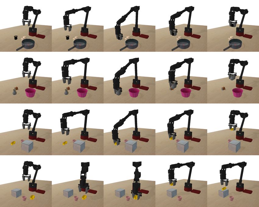
Under review as a conference paper at ICLR 2021

                Grasp cup                                                 Put candle in
                                                                               tray

                  ...

                                                                               ...
              Place bottle on
                   cube
    Scene 1                                                  Scene N       Pick vase

 Training Data

    Policy                      Prior

                                                       Exploration & RL: Use our behavioral prior to learn a specific task via RL.
                                                                       For example, pick and place the chair.

Figure 1: Our problem setting. Our training dataset consists of near-optimal state-action trajectories (without
reward labels) from a wide range of tasks. Each task might involve interacting with a different set of objects.
Even for the same set of objects, the task can be different depending on our objective. For example, in the
upper right corner, the objective could be picking up a cup, or it could be to place the bottle on the yellow cube.
We learn a behavioral prior from this multi-task dataset capable of trying many different useful behaviors when
placed in a new environment, and can aid an RL agent to quickly learn a specific task in this new environment.

from a unit Gaussian, and use the learned mappingTransfer   (which we refer to as the behavioral prior) to
generate likely environment actions, conditional onBehavioral
                                                            the
                                                            Prior
                                                                  current observation. This learned mapping
essentially transforms the original MDP into a simpler
                                                   Trial 1                   Learning
                                                                one for the RL  agent,New  Tasks
                                                                                       as long as the original
MDP shares (partial) structure with previously seen MDPs (see Section 3). Furthermore, since this
mapping is invertible, the RL agent still retains full
                                                   Trial 2
                                                          control over the original MDP: for every possible
environment action, there exists a point within the support of the Gaussian distribution that maps to
that action. This allows the RL agent to still try out new behaviors that are distinct from what was
previously observed.                              Trial n-1

Our main contribution is a framework for pre-training in RL from a diverse multi-task dataset, which
                                                  Trial n
produces a behavioral prior that accelerates acquisition   of new skills. We present an instantiation
of this framework in robotic manipulation, where we utilize manipulation data from a diverse range
of prior tasks to train our behavioral prior, and then use it to bootstrap exploration for new tasks.
By making it possible to pre-train action representations on large prior datasets for robotics and RL,
we hope that our method provides a path toward leveraging large datasets in the RL and robotics
settings, much like language models can leverage large text corpora in NLP and unsupervised pre-
training can leverage large image datasets in computer vision. Our method, which we call Prior
AcceleRated ReinfOrcemenT (PARROT), is able to quickly learn tasks that involve manipulating
previously unseen objects, from image observations and sparse rewards, in settings where RL from
scratch fails to learn a policy at all. We also compare against prior works that incorporate prior data
for RL, and show that PARROT substantially outperforms these prior works.

2     R ELATED W ORK
Combining RL with demonstrations. Our work is related to methods for learning from demon-
strations (Pomerleau, 1989; Schaal et al., 2003; Ratliff et al., 2007; Pastor et al., 2009; Ho & Ermon,
2016; Finn et al., 2017b; Giusti et al., 2016; Sun et al., 2017; Zhang et al., 2017; Lynch et al., 2019).
While demonstrations can also be used to speed up RL (Schaal, 1996; Peters & Schaal, 2006; Ko-
rmushev et al., 2010; Hester et al., 2017; Vecerı́k et al., 2017; Nair et al., 2018; Rajeswaran et al.,
2018; Silver et al., 2018; Peng et al., 2018; Johannink et al., 2019; Gupta et al., 2019), this usually
requires collecting demonstrations for the specific task that is being learned. In contrast, we use
data from a wide range of other prior tasks to speed up RL for a new task. As we show in our
experiments, PARROT is better suited to this problem setting when compared to prior methods that
combine imitation and RL for the same task.
Generative modeling and RL. Several prior works model multi-modal action distributions using
expert trajectories from different tasks. IntentionGAN (Hausman et al.) and InfoGAIL (Li et al.,
2017) learn multi-modal policies via interaction with an environment using an adversarial imitation
approach (Ho & Ermon, 2016), but we learn these distributions only from data. Other works learn
these distributions from data (Xie et al., 2019; Rhinehart et al., 2020) and utilize them for planning

                                                        2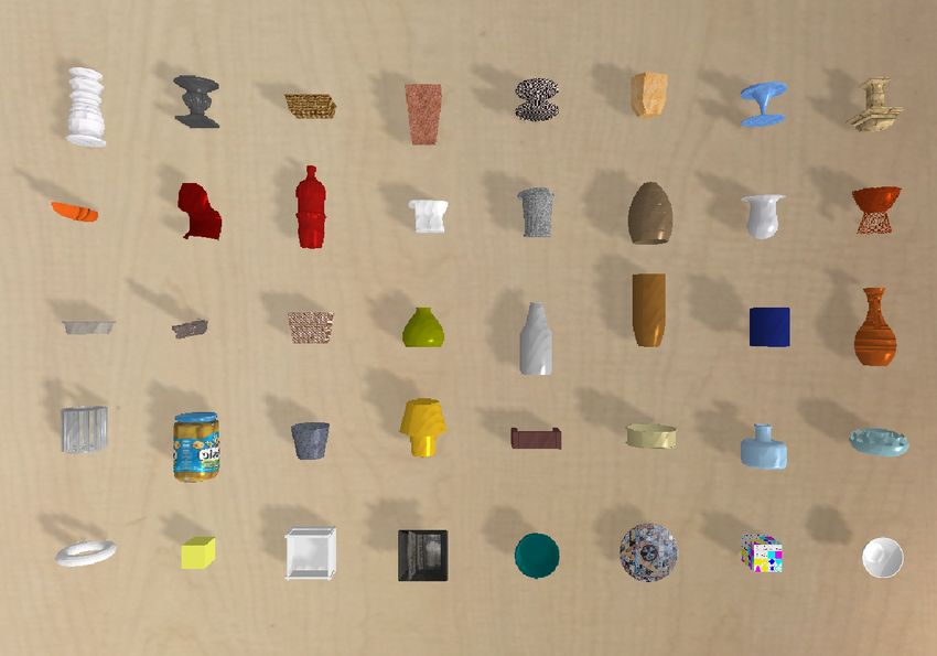
Under review as a conference paper at ICLR 2021

at test time to optimize a user-provided cost function. In contrast, we use the behavioral prior to
augment model-free RL of a new task. This allows us to learn policies for new tasks that may be
substantially different from prior tasks, since we can collect data specific to the new task at hand, and
we do not explicitly need to model the environment, which can be complicated for high-dimensional
state and action spaces, such as when performing continuous control from images observations.
Another line of work (Ghadirzadeh et al., 2017; Hämäläinen et al., 2019; Ghadirzadeh et al., 2020)
explores using generative models for RL, using a variational autoencoder (Kingma & Welling, 2014)
to model entire trajectories in an observation-independent manner, and then learning an open-loop,
single-step policy using RL to solve the downstream task. Our approach differs in several key
aspects: (1) our model is observation-conditioned, allowing it to prioritize actions that are relevant
to the current scene or environment, (2) our model allows for closed-loop feedback control, and (3)
our model is invertible, allowing the high-level policy to retain full control over the action space.
Our experiments demonstrate these aspects are crucial for solving harder tasks.
Hierarchical learning. Our method can be interpreted as training a hierarchical model: the low-
level policy is the behavioral prior trained on prior data, while the high-level policy is trained us-
ing RL and controls the low-level policy. This structure is similar to prior work in hierarchical
RL (Dayan & Hinton, 1992; Parr & Russell, 1997; Dietterich, 1998; Sutton et al., 1999; Kulka-
rni et al., 2016). We divide prior work in hierarchical learning into two categories: methods that
seek to learn both the low-level and high-level policies through active interaction with an environ-
ment (Kupcsik et al., 2013; Heess et al., 2016; Bacon et al., 2017; Florensa et al., 2017; Haarnoja
et al., 2018a; Nachum et al., 2018; Chandak et al., 2019; Peng et al., 2019), and methods that learn
temporally extended actions, also known as options, from demonstrations, and then recompose them
to perform long-horizon tasks through RL or planning (Fox et al., 2017; Krishnan et al., 2017; Kipf
et al., 2019; Shankar et al., 2020; Shankar & Gupta, 2020). Our work shares similarities with the
data-driven approach of the latter methods, but work on options focuses on modeling the temporal
structure in demonstrations for a small number of long-horizon tasks, while our behavioral prior is
not concerned with temporally-extended abstractions, but rather with transforming the original MDP
into one where potentially useful behaviors are more likely, and useless behaviors are less likely.
Meta-learning. Our goal in this paper is to utilize data from previously seen tasks to speed up RL
for new tasks. Meta-RL (Duan et al., 2016; Wang et al., 2016; Finn et al., 2017a; Mishra et al.,
2017; Rakelly et al., 2019; Mendonca et al., 2019; Zintgraf et al., 2020; Fakoor et al., 2020) and
meta-imitation methods (Duan et al., 2017; Finn et al., 2017c; Huang et al., 2018; James et al.,
2018; Paine et al., 2018; Yu et al., 2018; Huang et al., 2019; Zhou et al., 2020) also seek to speed
up learning for new tasks by leveraging experience from previously seen tasks. While meta-learning
provides an appealing and principled framework to accelerate acquisition of future tasks, we focus
on a more lightweight approach with relaxed assumptions that make our method more practically
applicable, and we discuss these assumptions in detail in the next section.

3    P ROBLEM S ETUP

Our goal is to improve an agent’s ability to learn new tasks by incorporating a behavioral prior,
which it can acquire from previously seen tasks. Each task can be considered a Markov decision
process (MDP), which is defined by a tuple (S, A, T, r, γ), where S and A represent state and
action spaces, T(s0 |s, a) and r(s, a) represent the dynamics and reward functions, and γ ∈ (0, 1)
represents the discount factor. Let p(M ) denote a distribution over such MDPs, with the constraint
that the state and action spaces are fixed. In our experiments, we treat high-dimensional images as s,
which means that this constraint is not very restrictive in practice. In order for the behavioral prior to
be able to accelerate the acquisition of new skills, we assume the behavioral prior is trained on data
that structurally resembles potential optimal policies for all or part of the new task. For example,
if the new task requires placing a bottle in a tray, the prior data might include some behaviors that
involve picking up objects. There are many ways to formalize this assumption. One way to state
this formally is to assume that prior data consists of executions of near-optimal policies for MDPs
drawn according to M ∼ p(M ), and the new task M ? is likewise drawn from p(M ). In this case,
the generative process for the prior data can be expressed as:

                  M ∼ p(M ),       πM (τ ) = arg max Eπ,M [RM ],       τM ∼ πM (τ ),                  (1)
                                                    π

                                                    3
Under review as a conference paper at ICLR 2021

            Transformed MDP                 Behavioral Prior                                        Data from
                                                                                                        many
                                                                                                        tasks

                                 Image observation   Convolutional Neural
                                                          Network

                                         noise

RL Policy
                 Original MDP

Figure 2: PARROT. Using successful trials from a large variety of tasks, we learn an invertible mapping fφ
              s
that maps noise      z to useful actions a. This mappingZ0is conditioned on
                                                                         Z1              Z2
                                                                            the current observation,    Z3=a
                                                                                                     which in our
case is an RGB image. The image is passed through a stack of convolutional layers and flattened to obtain
an image encoding
                f(z; s)
                        ψ(s), and this image encoding is then used to condition each individual transformation fi
        overall mapping function fφ . The parameters of the mapping (including the convolutional encoder) are
of ourpi(z|s)
learned through maximizing thea conditional log-likelihood of state-action pairs observed in the dataset. When
learning a new task, this mapping can simplify the MDP for an RL agent by mapping actions sampled from a
randomly initialized policy to actions that are likely to lead to useful behavior in the current scene. Since the
mapping is invertible, the RL agent still retains full control over the action space of the original MDP, simply
the likelihood of executing a useful action is increased through use of the pre-trained mapping.

where τM = (s1 , a1 , s2 , a2 , . . . , sT , aT ) is a sequence of state P
                                                                         and actions, πM (τ ) denotes a near-
                                                                           ∞
optimal policy (Kearns & Singh, 2002) for MDP M and RM = t=0 γ t rt . When incorporating the
                                                    ?
behavioral prior for learning a new task M , our goal is the same as standard RL: to find a policy π
that maximizes the expected return arg maxπ Eπ,M ? [RM ? ]. Our assumption on tasks being drawn
from a distribution p(M ) shares similarities with the meta-RL problem (Wang et al., 2016; Duan
et al., 2016), but our setup is different: it does not require accessing any task in p(M ) except the
new task we are learning, M ? . Meta-RL methods need to interact with the tasks in p(M ) during
meta-training, with access to rewards and additional samples, whereas we learn our behavioral prior
simply from data, without even requiring this data to be labeled with rewards. This is of particular
importance for real-world problem settings such as robotics: it is much easier to store data from
prior tasks (e.g., different environments) than to have a robot physically revisit those prior settings
and retry those tasks, and not requiring known rewards makes it possible to use data from a variety
of sources, including human-provided demonstrations. In our setting, RL is performed in only one
environment, while the prior data can come from many environments.
Our setting is related to meta-imitation learning (Duan et al., 2017; Finn et al., 2017c), as we
speed up learning new tasks using data collected from past tasks. However, meta-imitation learning
methods require at least one demonstration for each new task, whereas our method can learn new
tasks without any demonstrations. Further, our data requirements are less stringent: meta-imitation
learning methods require all demonstrations to be optimal, require all trajectories in the dataset to
have a task label, and requires “paired demonstrations”, i.e. at least two demonstrations for each
task (since meta-imitation methods maximize the likelihood of actions from one demonstration after
conditioning the policy on another demonstration from the same task). Relaxing these requirements
increases the scalability of our method: we can incorporate data from a wider range of sources, and
we do not need to explicitly organize it into specific tasks.

4    B EHAVIORAL P RIORS F OR R EINFORCEMENT L EARNING

Our method learns a behavioral prior for downstream RL by utilizing a dataset D of (near-optimal)
state-action pairs from previously seen tasks. We do so by learning a state-conditioned mapping
fφ : Z × S → A (where φ denotes learnable parameters) that transforms a noise vector z into
an action a that is likely to be useful in the current state s. This removes the need for exploring
via “meaningless” random behavior, and instead enables an exploration process where the agent
attempts behaviors that have been shown to be useful in previously seen domains. For example, if a
robotic arm is placed in front of several objects, randomly sampling z (from a simple distribution,
such as the unit Gaussian) and applying the mapping a = fφ (z; s) should result in actions that,
when executed, result in meaningful interactions with the objects. This learned mapping essentially

                                                                  4
Under review as a conference paper at ICLR 2021

transforms the MDP experienced by the RL agent into a simpler one, where every random action
executed in this transformed MDP is much more likely to lead to a useful behavior.
How can we learn such a mapping? In this paper, we propose to learn this mapping through state-
conditioned generative modeling of the actions observed in the original dataset D, and we refer to
this state-conditioned distribution over actions as the behavioral prior pprior (a|s). A deep generative
model takes noise as input, and outputs a plausible sample from the target distribution, i.e. it can
represent pprior (a|s) as a distribution over noise z using a deterministic mapping fφ : Z × S 7→ A
When learning a new task, we can use this mapping to reparametrize the action space of the RL
agent: if the action chosen by the randomly initialized neural network policy is z, then we execute
the action a = fφ (z; s) in the original MDP, and learn a policy π(z|s) that maximizes the task reward
through learning to control the inputs to the mapping fφ . The training of the behavioral prior and
the task-specific policy is decoupled, allowing us to mix and match RL algorithms and generative
models to best suit the application of interest. An overview of our overall architecture is depicted in
Figure 2. In the next subsection, we discuss what properties we would like the behavioral prior to
satisfy, and present one particular choice for learning a prior that satisfies all of these properties.

4.1   L EARNING A B EHAVIORAL P RIOR W ITH N ORMALIZING F LOWS

For the behavioral prior to be effective, it needs to satisfy certain properties. Since we learn the
prior from a multi-task dataset, containing several different behaviors even for the same initial state,
the learned prior should be capable of representing complex, multi-modal distributions. Second,
it should provide a mapping for generating “useful” actions from noise samples when learning a
new task. Third, the prior should be state-conditioned, so that only actions that are relevant to the
current state are sampled. And finally, the learned mapping should allow easier learning in the
reparameterized action space without hindering the RL agent’s ability to attempt novel behaviors,
including actions that might not have been observed in the dataset D. Generative models based
on normalizing flows (Dinh et al., 2017) satisfy all of these properties well: they allow maximizing
the model’s exact log-likelihood of observed examples, and learn a deterministic, invertible mapping
that transforms samples from a simple distribution pz to examples observed in the training dataset. In
particular, the real-valued non-volume preserving (real NVP) architecture introduced by Dinh et al.
(2017) allows using deep neural networks to parameterize this mapping (making it expressive) While
the original real NVP work modelled unconditional distributions, follow-up work has found that it
can be easily extended to incorporate conditioning information (Ardizzone et al., 2019). We refer the
reader to prior work (Dinh et al., 2017) for a complete description of real NVPs, and summarize its
key features here. Given an invertible mapping a = fφ (z; s), the change of variable formula allows
expressing the likelihood of the observed actions using samples from D in the following way:
                           pprior (a|s) = pz fφ−1 (a; s) det ∂fφ (a;s)/∂a
                                                                −1

                                                                                                     (2)
Dinh et al. (2017) propose a particular (unconditioned) form of the invertible mapping fφ , called an
affine coupling layer, that maintains tractability of the likelihood term above, while still allowing the
mapping fφ to be expressive. Several coupling layers can be composed together to transform simple
noise vectors into samples from complex distributions, and each layer can be conditioned on other
variables, as shown in Figure 2.

4.2   ACCELERATED R EINFORCEMENT L EARNING VIA B EHAVIORAL P RIORS

After we obtain the mapping fφ (z; s) from the behavioral prior learned by maximizing the likelihood
term in Equation 2, we would like to use it to accelerate RL when solving a new task. Instead of
learning a policy πθ (a|s) that directly executes its actions in the original MDP, we learn a policy
πθ (z|s), and execute an action in the environment according to a = fφ (z; s). As shown in Figure 2,
this essentially transforms the MDP experienced for the RL agent into one where random actions
z ∼ pz (where pz is the base distribution used for training the mapping fφ ) are much more likely
to result in useful behaviors. To enable effective exploration at the start of the learning period, we
initialize the RL policy to the base distribution used for training the prior, so that at the beginning of
training, πθ (z|s) := pz (z). Since the mapping fφ is invertible, the RL agent still retains full control
over the action space: for any given a, it can always find a z that generates z = fφ−1 (a; s) in the
original MDP. The learned mapping increases the likelihood of useful actions without crippling the
RL agent, making it ideal for fine-tuning from task-specific data. Our complete method is described

                                                    5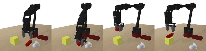
Under review as a conference paper at ICLR 2021
in Algorithm 1 in Appendix A. Note that we need to learn the mapping fφ only once, and it can be
used for accelerated learning of any new task.
4.3 I MPLEMENTATION D ETAILS
We use real NVP to learn fφ , and as shown in Figure 2, each coupling layer in the real NVP takes
as input the the output of the previous coupling layer, and the conditioning information. The con-
ditioning information in our case corresponds to RGB image observations, which allows us to train
a single behavioral prior across a wide variety of tasks, even when the tasks might have different
underlying states (for example, different objects). We train a real NVP model with four coupling
layers; the exact architecture, and other hyperparameters, are detailed in Appendix B. The behav-
ioral prior can be combined with any RL algorithm that is suitable for continuous action spaces, and
we chose to use the soft actor-critic (Haarnoja et al., 2018b) due to its stability and ease of use.
5 E XPERIMENTS
Our experiments seek to answer: (1) Can the behavioral prior accelerate learning of new tasks? (2)
How does PARROT compare to prior works that accelerate RL with demonstrations? (3) How does
PARROT compare to prior methods that combine hierarchical imitation with RL?
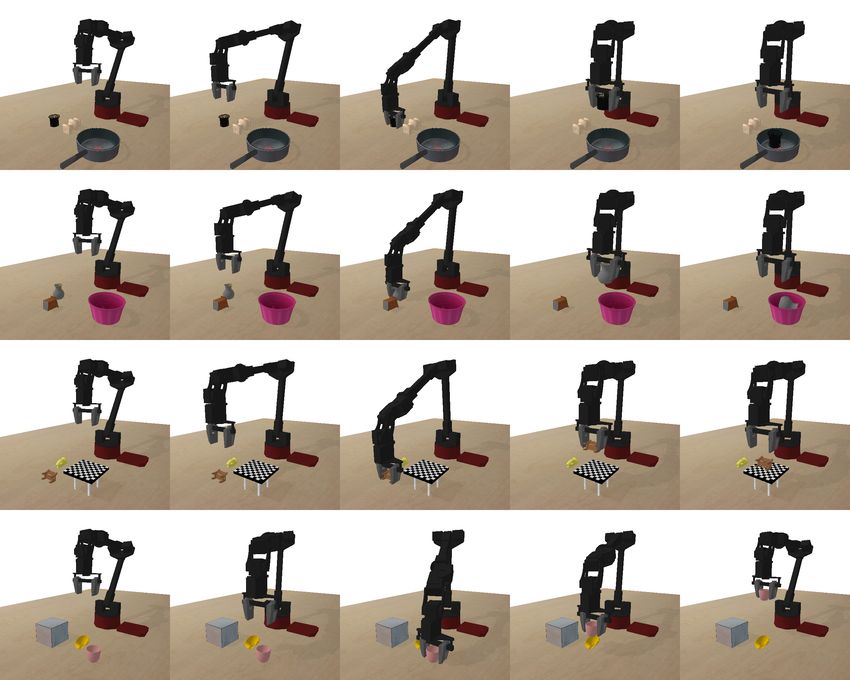
Domains. We evaluate our method on a suite of
challenging robotic manipulation tasks, a subset of
which are depicted in Figure 3. Each task involves
controlling a 6-DoF robotic arm and its gripper,
with a 7D action space. The observation is a 48×48
RGB image, which allows us to use the same ob-
servation representation across tasks, even though
each underlying task might have a different under-
lying state (e.g., different objects). No other obser-
vations (such as joint angles or end-effector posi-
tions) are provided. In each task, the robot needs
to interact with one or two objects in the scene to
achieve its objective, and there are three objects in
each scene. Note that all of the objects in the test
scenes are novel – the dataset D contains no inter-
actions with these objects. The object positions at Figure 3: Tasks. A subset of our evaluation tasks,
the start of each trial are randomized, and the policy with one task shown in each row. In the first task
(first row), the objective is to pick up a can and
must infer these positions from image observations place it in the pan. In the second task, the robot
in order to successfully solve the task. A reward must pick up the vase and put it in the basket. In
of +1 is provided when the objective for the task the third task, the goal is to place the chair on top of
is achieved, and the reward is zero otherwise. De- the checkerboard. In the fourth task, the robot must
tailed information on the objective for each task and pick up the mug and hold it above a certain height.
example rollouts are provided in Appendix C.1, and Initial positions of all objects are randomized, and
on our anonymous project website1 . must be inferred from visual observations. Not all
objects in the scene are relevant to the current task.
Data collection. Our behavioral prior is trained on
a diverse dataset of trajectories from a wide range
of tasks, and then utilized to accelerate reinforcement learning of new tasks. As discussed in Sec-
tion 3, for the prior to be effective, it needs to be trained on a dataset that structurally resembles the
behaviors that might be optimal for the new tasks. In our case, all of the behaviors involve reposi-
tioning objects (i.e., picking up objects and moving them to new locations), which represents a very
general class of tasks that might be performed by a robotic arm. While the dataset can be collected
in many ways, such as from human demonstrations or prior tasks solved by the robot, we collect it
using a set of randomized scripted policies, see Appendix C.2 for details. Since the policies are ran-
domized, not every execution of such a policy results in a useful behavior, and we decide to keep or
discard a collected trajectory based on a simple predefined rule: if the trajectory collected ends with
a successful grasp or rearrangement of any one of the objects in the scene, we add this trajectory to
1
https://sites.google.com/view/prior-parrot
6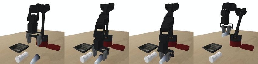
Under review as a conference paper at ICLR 2021

our dataset. We collect a dataset of 50K trajectories, where each trajectory is of length 25 timesteps
(≈5-6 seconds), for a total of 1.25m observation-action pairs. The observation is a 48 × 48 RGB
image, while the actions are continuous 7D vectors. Data collection involves interactions with over
50 everyday objects (see Appendix C.3); the diversity of this dataset enables learning priors that can
produce useful behavior when interacting with a new object.

5.1   R ESULTS , C OMPARISONS AND A NALYSIS

To answer the questions posed at the start of this section, we compare PARROT against a number
of prior works, as well as ablations of our method. Additional implementation details and hyperpa-
rameters can be found in Appendix B.
Soft-Actor Critic (SAC). For a basic RL comparison, we compare against the vanilla soft-actor
critic algorithm (Haarnoja et al., 2018b), which does not incorporate any previously collected data.
SAC with demonstrations (BC-SAC). We compare against a method that incorporates demonstra-
tions to speed up learning of new tasks. In particular, we initialize the SAC policy by performing
behavioral cloning on the entire dataset D, and then fine-tune it using SAC. This approach is similar
to what has been used in prior work (Rajeswaran et al., 2018), except we use SAC as our RL algo-
rithm. While we did test other methods that are designed to use demonstration data with RL such as
DDPGfD (Vecerı́k et al., 2017) and AWAC (Nair et al., 2020), we found that our simple BC + SAC
variant performed better. This somewhat contradicts the results reported in prior work (Nair et al.,
2020), but we believe that this is because the prior data is not labeled with rewards (all transitions
are assigned a reward of 0), and more powerful demonstration + RL methods require access to these
rewards, and subsequently struggle due to the reward misspecification.
Transfer Learning via Feature Learning (VAE-features). We compare against prior methods
for transfer learning (in RL) that involve learning a robust representation of the input observation.
Similar to Higgins et al. (2017b), we train a β-VAE using the observations in our training set, and
train a policy on top of the features learned by this VAE when learning downstream tasks.
Trajectory modeling and RL (TrajRL). Ghadirzadeh et al. (2020) model entire trajectories using
a VAE, and learn a one-step policy on top of the VAE to solve tasks using RL. Our implementation
of this method uses a VAE architecture identical to the original paper’s, and we then train a policy
using SAC to solve new tasks with the action space induced by the VAE. We performed additional
hyperparameter tuning for this comparison, the details of which can be found in Appendix B.
Hierarchical imitation and RL (HIRL). Prior
works in hierarchical imitation learning (Fox et al.,
2017; Shankar & Gupta, 2020) train latent variable
models over expert demonstrations to discover op-
tions, and later utilize these options to learn long-
horizon tasks using RL. While PARROT can also be
extended to model the temporal structure in trajecto-
ries through conditioning on past states and actions,
by modeling pprior (at , |st , st−1 , ..., at−1 , ..., a0 ) in-
stead of pprior (at |st ), we focus on a simpler version
of the model in this paper that does not condition
on the past. In order to provide a fair comparison, Figure 4: We plot trajectories from executing a
we modify the model proposed by Shankar & Gupta random policy, with and without the behavioral
(2020) to remove the past conditioning, which then prior. We see that the behavioral prior substan-
reduces to training a conditional VAE, and perform- tially increases the likelihood of executing an ac-
ing RL on the action space induced by the latent tion that is likely to lead to a meaningful interac-
space of this VAE. This comparison is similar to our tion with an object, while still exploring a diverse
proposed approach, but with one crucial difference: set of actions.
the mapping we learn is invertible, and allows the
RL agent to retain full control over the final actions in the environment (since for every a ∈ A, there
exist some z = fφ−1 (a; s), while a latent space learned by a VAE provides no such guarantee).
Exploration via behavioral prior (Prior-explore). We also run experiments with an ablation of
our method: instead of using a behavioral prior to transform the MDP being experienced by the RL

                                                   7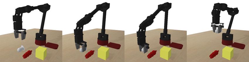
Under review as a conference paper at ICLR 2021

                  1.0
                               Place Can in Pan                           1.0
                                                                                     Place Sculpture in Basket                      Place Chair on Checkerboard Table
                                                                                                                                    1.0                                                      1.0
                                                                                                                                                                                                        Place Baseball Cap on Block

                  0.8                                                     0.8                                                       0.8                                                      0.8

   Success Rate

                                                           Success Rate

                                                                                                                     Success Rate

                                                                                                                                                                              Success Rate
                  0.6                                                     0.6                                                       0.6                                                      0.6

                  0.4                                                     0.4                                                       0.4                                                      0.4

                  0.2                                                     0.2                                                       0.2                                                      0.2

                  0.0                                                     0.0                                                       0.0                                                      0.0
                        0K   100K   200K   300K   400K   500K                   0K    100K   200K   300K   400K    500K                   0K   100K    200K   300K   400K   500K                   0K      100K   200K   300K   400K   500K
                                    Timesteps                                               Timesteps                                                  Timesteps                                                Timesteps
                  1.0
                                    Pick up Bar                           1.0
                                                                                        Pick Up Sculpture                           1.0
                                                                                                                                                      Pick up Cup                            1.0
                                                                                                                                                                                                           Pick up Baseball Cap

                  0.8                                                     0.8                                                       0.8                                                      0.8
   Success Rate

                                                           Success Rate

                                                                                                                     Success Rate

                                                                                                                                                                              Success Rate
                  0.6                                                     0.6                                                       0.6                                                      0.6

                  0.4                                                     0.4                                                       0.4                                                      0.4

                  0.2                                                     0.2                                                       0.2                                                      0.2

                  0.0                                                     0.0                                                       0.0                                                      0.0
                        0K   100K   200K   300K   400K   500K                   0K    100K   200K   300K   400K    500K                   0K   100K    200K   300K   400K   500K                   0K      100K   200K   300K   400K   500K
                                  Timesteps                                                  Timesteps                                                Timesteps                                                  Timesteps
                                PARROT (ours)                  BC+SAC                          SAC                HIRL                         TrajRL         VAE-features                                 Prior-explore

Figure 5: Results. The lines represent average performance across multiple random seeds, and the shaded
areas represent the standard deviation. PARROT is able to learn much faster than prior methods on a majority
of the tasks, and shows little variance across runs (all experiments were run with three random seeds, compu-
tational constraints of image-based RL make it difficult to run more seeds). Note that some methods that failed
to make any progress on certain tasks (such as “Place Sculpture in Basket”) overlap each other with a success
rate of zero. SAC and VAE-features fail to make progress on any of the tasks.

agent, we use it to simply aid the exploration process. While collecting data, an action is executed
from the prior with probability , else an action is executed from the learned policy. We experimented
with  = 0.1, 0.3, 0.7, 0.9, and found 0.9 to perform best.
Main results. Our results are summarised in Figure 5. We see that PARROT is able to solve all
of the tasks substantially faster and achieve substantially higher final returns than other methods.
The SAC baseline (which does not use any prior data) fails to make progress on any of the tasks,
which we suspect is due to the challenge of exploring in sparse reward settings with a randomly
initialized policy. Figure 4 illustrates a comparison between using a behavioral prior and a random
policy for exploration. The VAE-features baseline similarly fails to make any progress, and due to
the same reason: the difficulty of exploration in a sparse reward setting. Initializing the SAC policy
with behavior cloning allows it to make progress on only two of the tasks, which is not surprising:
a Gaussian policy learned through a behavior cloning loss is not expressive enough to represent the
complex, multi-modal action distributions observed in dataset D. Both TrajRL and HIRL perform
much better than any of the other baselines, but their performance plateaus a lot earlier than PAR-
ROT. While the initial exploration performance of our learned behavioral prior is not substantially
better from these methods (denoted by the initial success rate in the learning curves), the flexibility
of the representation it offers (through learning an invertible mapping) allows the RL agent to im-
prove far beyond its initial performance. Prior-explore, an ablation of our method, is able to make
progress on most tasks, but is unable to learn as fast as our method, and also demonstrates unstable
learning on some of the tasks. We suspect this is due to the following reason: while off-policy RL
methods like SAC aim to learn from data collected by any policy, they are in practice quite sensitive
to the data distribution, and can run into issues if the data collection policy differs substantially from
the policy being learned (Kumar et al., 2019).
Impact of dataset size on performance. We conducted additional experiments on a subset of
our tasks to evaluate how final performance is impacted as a result of dataset size, results from
which are shown in Figure 6. As one might expect, the size of the dataset positively correlates
with performance, but about 10K trajectories are sufficient for obtaining good performance, and
collecting additional data yields diminishing returns. Note that initializing with even a smaller
dataset size (like 5K trajectories) yields much better performance than learning from scratch.

                                                                                                                   8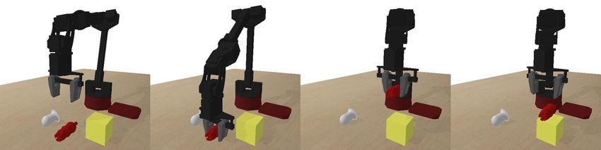
Under review as a conference paper at ICLR 2021

                                 Pick up Cup                            1.0
                                                                                   Pick up Baseball Cap                                       Pick Up Sculpture                          1.0
                                                                                                                                                                                                           Pick up Bar
               1.0                                                                                                               1.0

               0.8                                                      0.8                                                      0.8                                                     0.8
Success Rate

                                                         Success Rate

                                                                                                                  Success Rate

                                                                                                                                                                          Success Rate
               0.6                                                      0.6                                                      0.6                                                     0.6

               0.4                                                      0.4                                                      0.4                                                     0.4

               0.2                                                      0.2                                                      0.2                                                     0.2

               0.0                                                      0.0                                                      0.0                                                     0.0
                     0K   100K    200K   300K   400K   500K                   0K   100K    200K   300K   400K   500K                   0K   100K   200K   300K   400K   500K                   0K   100K   200K   300K   400K   500K
                                 Timesteps                                                 Timesteps                                               Timesteps                                               Timesteps
                                                                                          5K         10K                         25K                50K

 Figure 6: Impact of dataset size on performance. We observe that training on 10K, 25K or 50K trajectories
 yields similar performance.

 Mismatch between train and test tasks. We
 ran experiments in which we deliberately bias
 the training dataset so that the training tasks and
 test tasks are functionally different (i.e. involve
 substantially different actions), the results from
 which are shown in Figure 7. We observe that
 if the prior is trained on pick and place tasks
 alone, it can still solve downstream grasping
 tasks well. However, if the prior is trained only
 on grasping, it is unable to perform well when
 solving pick and place tasks. We suspect this
 is due to the fact that pick and place tasks in-                                                                     Figure 7: Impact of train/test mismatch on perfor-
 volve a completely new action (that of open-                                                                         mance. Each plot shows results for four tasks. Note
 ing the gripper), which is never observed by the                                                                     that for the pick and place tasks, the performance is
 prior if it is trained only on grasping, making it                                                                   close to zero, and the curves mostly overlap each other
 difficult to learn this behavior from scratch for                                                                    on the x-axis.
 downstream tasks.

  6                   C ONCLUSION
 We presented PARROT, a method for learning behavioral priors using successful trials from a wide
 range of tasks. Learning from priors accelerates RL on new tasks–including manipulating previously
 unseen objects from high-dimensional image observations–which RL from scratch often fails to
 learn. Our method also compares favorably to other prior works that use prior data to bootstrap
 learning for new tasks. While our method learns faster and performs better than prior work in
 learning novel tasks, it still requires thousands of trials to attain high success rates. Improving this
 efficiency even further, perhaps inspired by ideas in meta-learning, could be a promising direction
 for future work. Our work opens the possibility for several exciting future directions. PARROT
 provides a mapping for executing actions in new environments structurally similar to those of prior
 tasks. While we primarily utilized this mapping to accelerate learning of new tasks, future work
 could investigate how it can also enable safe exploration of new environments (Hunt et al., 2020;
 Rhinehart et al., 2020). While the invertibility of our learned mapping ensures that it is theoretically
 possible for the RL policy to execute any action in the original MDP, the probability of executing
 an action can become very low if this action was never seen in the training set. This can be an issue
 if there is a significant mismatch between the training dataset and the downstream task (as shown
 in our experiments), and tackling this issue would make for an interesting problem. Since our
 method speeds up learning using a problem setup that takes into account real world considerations
 (no rewards for prior data, no need to revisit prior tasks, etc.), we are also excited about its future
 application to domains like real world robotics.

                                                                                                                   9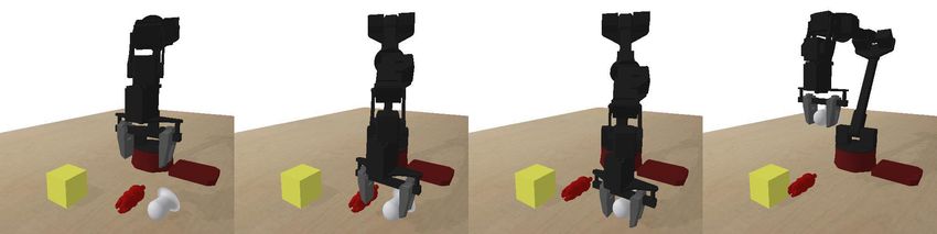
Under review as a conference paper at ICLR 2021

R EFERENCES
Lynton Ardizzone, Jakob Kruse, Carsten Rother, and Ullrich Köthe. Analyzing inverse problems
  with invertible neural networks. In ICLR, 2019.
Pierre-Luc Bacon, Jean Harb, and Doina Precup. The option-critic architecture. In AAAI, 2017.
Yash Chandak, Georgios Theocharous, James Kostas, Scott M. Jordan, and Philip S. Thomas. Learn-
  ing action representations for reinforcement learning. In ICML, 2019.
Angel X. Chang, Thomas A. Funkhouser, Leonidas J. Guibas, Pat Hanrahan, Qi-Xing Huang, Zimo
  Li, Silvio Savarese, Manolis Savva, Shuran Song, Hao Su, Jianxiong Xiao, Li Yi, and Fisher Yu.
  Shapenet: An information-rich 3d model repository. CoRR, abs/1512.03012, 2015.
E Coumans and Y Bai. Pybullet, a python module for physics simulation for games, robotics and
  machine learning. GitHub repository, 2016.
Peter Dayan and Geoffrey E. Hinton. Feudal reinforcement learning. In NIPS, 1992.
Jacob Devlin, Ming-Wei Chang, Kenton Lee, and Kristina Toutanova. BERT: pre-training of deep
  bidirectional transformers for language understanding. In NAACL-HLT, 2019.
Thomas G. Dietterich. The MAXQ method for hierarchical reinforcement learning. In ICML, 1998.
Laurent Dinh, Jascha Sohl-Dickstein, and Samy Bengio. Density estimation using real NVP. In
  ICLR, 2017.
Yan Duan, John Schulman, Xi Chen, Peter L Bartlett, Ilya Sutskever, and Pieter Abbeel. Rl2: Fast
  reinforcement learning via slow reinforcement learning. arXiv preprint arXiv:1611.02779, 2016.
Yan Duan, Marcin Andrychowicz, Bradly Stadie, Jonathan Ho, Jonas Schneider, Ilya Sutskever,
  Pieter Abbeel, and Wojciech Zaremba. One-shot imitation learning. Neural Information Process-
  ing Systems (NIPS), 2017.
Rasool Fakoor, Pratik Chaudhari, Stefano Soatto, and Alexander J. Smola. Meta-q-learning. In
  ICLR, 2020.
Chelsea Finn, Pieter Abbeel, and Sergey Levine. Model-agnostic meta-learning for fast adaptation
  of deep networks. arXiv preprint arXiv:1703.03400, 2017a.
Chelsea Finn, Sergey Levine, and Pieter Abbeel. Guided cost learning: Deep inverse optimal control
  via policy optimization. In International Conference on Machine Learning (ICML), 2017b.
Chelsea Finn, Tianhe Yu, Tianhao Zhang, Pieter Abbeel, and Sergey Levine. One-shot visual imita-
  tion learning via meta-learning. Conference on Robot Learning (CoRL), 2017c.
Carlos Florensa, Yan Duan, and Pieter Abbeel. Stochastic neural networks for hierarchical rein-
  forcement learning. In ICLR, 2017.
Roy Fox, Sanjay Krishnan, Ion Stoica, and Ken Goldberg. Multi-level discovery of deep options.
  CoRR, abs/1703.08294, 2017.
Ali Ghadirzadeh, Atsuto Maki, Danica Kragic, and Mårten Björkman. Deep predictive policy train-
  ing using reinforcement learning. In International Conference on Intelligent Robots and Systems,
  2017.
Ali Ghadirzadeh, Petra Poklukar, Ville Kyrki, Danica Kragic, and Mårten Björkman. Data-
  efficient visuomotor policy training using reinforcement learning and generative models. CoRR,
  abs/2007.13134, 2020.
Alessandro Giusti, Jérôme Guzzi, Dan C Cireşan, Fang-Lin He, Juan P Rodrı́guez, Flavio Fontana,
  Matthias Faessler, Christian Forster, Jürgen Schmidhuber, Gianni Di Caro, et al. A machine
  learning approach to visual perception of forest trails for mobile robots. IEEE Robotics and
  Automation Letters (RA-L), 2016.

                                               10
Under review as a conference paper at ICLR 2021
Abhishek Gupta, Vikash Kumar, Corey Lynch, Sergey Levine, and Karol Hausman. Relay policy
learning: Solving long-horizon tasks via imitation and reinforcement learning. In Leslie Pack
Kaelbling, Danica Kragic, and Komei Sugiura (eds.), Conference on Robot Learning, 2019.
Tuomas Haarnoja, Haoran Tang, Pieter Abbeel, and Sergey Levine. Reinforcement learning with
deep energy-based policies. In International Conference on Machine Learning (ICML), 2017.
Tuomas Haarnoja, Kristian Hartikainen, Pieter Abbeel, and Sergey Levine. Latent space policies for
hierarchical reinforcement learning. In Jennifer G. Dy and Andreas Krause (eds.), ICML, 2018a.
Tuomas Haarnoja, Aurick Zhou, Kristian Hartikainen, George Tucker, Sehoon Ha, Vikash Kumar
Jie Tan, Henry Zhu, Abhishek Gupta, Pieter Abbeel, and Sergey Levine. Soft actor-critic algo-
rithms and applications. Technical report, 2018b.
Aleksi Hämäläinen, Karol Arndt, Ali Ghadirzadeh, and Ville Kyrki. Affordance learning for end-
to-end visuomotor robot control. In IROS, 2019.
Karol Hausman, Yevgen Chebotar, Stefan Schaal, Gaurav S. Sukhatme, and Joseph J. Lim. Multi-
modal imitation learning from unstructured demonstrations using generative adversarial nets. In
Isabelle Guyon, Ulrike von Luxburg, Samy Bengio, Hanna M. Wallach, Rob Fergus, S. V. N.
Vishwanathan, and Roman Garnett (eds.), NIPS.
Nicolas Heess, Gregory Wayne, Yuval Tassa, Timothy P. Lillicrap, Martin A. Riedmiller, and David
Silver. Learning and transfer of modulated locomotor controllers. CoRR, abs/1610.05182, 2016.
Todd Hester, Matej Vecerı́k, Olivier Pietquin, Marc Lanctot, Tom Schaul, Bilal Piot, Andrew
Sendonaris, Gabriel Dulac-Arnold, Ian Osband, John P. Agapiou, Joel Z. Leibo, and Au-
drunas Gruslys. Learning from demonstrations for real world reinforcement learning. CoRR,
abs/1704.03732, 2017.
Irina Higgins, Loı̈c Matthey, Arka Pal, Christopher Burgess, Xavier Glorot, Matthew Botvinick,
Shakir Mohamed, and Alexander Lerchner. beta-vae: Learning basic visual concepts with a
constrained variational framework. In ICLR, 2017a.
Irina Higgins, Arka Pal, Andrei A. Rusu, Loı̈c Matthey, Christopher Burgess, Alexander Pritzel,
Matthew Botvinick, Charles Blundell, and Alexander Lerchner. DARLA: improving zero-shot
transfer in reinforcement learning. In ICML, 2017b.
Jonathan Ho and Stefano Ermon. Generative adversarial imitation learning. In Advances in Neural
Information Processing Systems (NIPS), 2016.
De-An Huang, Suraj Nair, Danfei Xu, Yuke Zhu, Animesh Garg, Li Fei-Fei, Silvio Savarese, and
Juan Carlos Niebles. Neural task graphs: Generalizing to unseen tasks from a single video demon-
stration. 2018.
De-An Huang, Danfei Xu, Yuke Zhu, Animesh Garg, Silvio Savarese, Li Fei-Fei, and Juan Carlos
Niebles. Continuous relaxation of symbolic planner for one-shot imitation learning. In IROS,
2019.
Nathan Hunt, Nathan Fulton, Sara Magliacane, Nghia Hoang, Subhro Das, and Armando
Solar-Lezama. Verifiably safe exploration for end-to-end reinforcement learning. CoRR,
abs/2007.01223, 2020.
Sergey Ioffe and Christian Szegedy. Batch normalization: Accelerating deep network training by
reducing internal covariate shift. In ICML, 2015.
Stephen James, Michael Bloesch, and Andrew J Davison. Task-embedded control networks for
few-shot imitation learning. arXiv preprint arXiv:1810.03237, 2018.
Tobias Johannink, Shikhar Bahl, Ashvin Nair, Jianlan Luo, Avinash Kumar, Matthias Loskyll,
Juan Aparicio Ojea, Eugen Solowjow, and Sergey Levine. Residual reinforcement learning for
robot control. In ICRA, 2019.
11Under review as a conference paper at ICLR 2021
Michael J. Kearns and Satinder P. Singh. Near-optimal reinforcement learning in polynomial time.
Machine Learning, 49(2-3):209–232, 2002.
Diederik P. Kingma and Jimmy Ba. Adam: A method for stochastic optimization. In International
Conference for Learning Representations (ICLR), 2015.
Diederik P. Kingma and Max Welling. Auto-encoding variational bayes. In Yoshua Bengio and
Yann LeCun (eds.), ICLR, 2014.
Thomas Kipf, Yujia Li, Hanjun Dai, Vinı́cius Flores Zambaldi, Alvaro Sanchez-Gonzalez, Edward
Grefenstette, Pushmeet Kohli, and Peter W. Battaglia. Compile: Compositional imitation learning
and execution. In Kamalika Chaudhuri and Ruslan Salakhutdinov (eds.), ICML, 2019.
Petar Kormushev, Sylvain Calinon, and Darwin G. Caldwell. Robot motor skill coordination with
em-based reinforcement learning. In IROS, 2010.
Sanjay Krishnan, Roy Fox, Ion Stoica, and Ken Goldberg. DDCO: discovery of deep continuous
options for robot learning from demonstrations. In CoRL, 2017.
Tejas D. Kulkarni, Karthik Narasimhan, Ardavan Saeedi, and Josh Tenenbaum. Hierarchical deep
reinforcement learning: Integrating temporal abstraction and intrinsic motivation. In Advances in
Neural Information Processing Systems, 2016.
Aviral Kumar, Justin Fu, Matthew Soh, George Tucker, and Sergey Levine. Stabilizing off-policy
q-learning via bootstrapping error reduction. In NeurIPS, 2019.
Andras Gabor Kupcsik, Marc Peter Deisenroth, Jan Peters, and Gerhard Neumann. Data-efficient
generalization of robot skills with contextual policy search. In AAAI, 2013.
Yunzhu Li, Jiaming Song, and Stefano Ermon. Infogail: Interpretable imitation learning from visual
demonstrations. In Advances in Neural Information Processing Systems, 2017.
Corey Lynch, Mohi Khansari, Ted Xiao, Vikash Kumar, Jonathan Tompson, Sergey Levine, and
Pierre Sermanet. Learning latent plans from play. In Conference on Robot Learning, 2019.
Russell Mendonca, Abhishek Gupta, Rosen Kralev, Pieter Abbeel, Sergey Levine, and Chelsea Finn.
Guided meta-policy search. arXiv preprint arXiv:1904.00956, 2019.
Nikhil Mishra, Mostafa Rohaninejad, Xi Chen, and Pieter Abbeel. Meta-learning with temporal
convolutions. arXiv:1707.03141, 2017.
Ofir Nachum, Shixiang Gu, Honglak Lee, and Sergey Levine. Data-efficient hierarchical reinforce-
ment learning. In Samy Bengio, Hanna M. Wallach, Hugo Larochelle, Kristen Grauman, Nicolò
Cesa-Bianchi, and Roman Garnett (eds.), Advances in Neural Information Processing Systems,
2018.
Ashvin Nair, Bob McGrew, Marcin Andrychowicz, Wojciech Zaremba, and Pieter Abbeel. Over-
coming exploration in reinforcement learning with demonstrations. In ICRA, 2018.
Ashvin Nair, Murtaza Dalal, Abhishek Gupta, and Sergey Levine. Accelerating online reinforcement
learning with offline datasets. CoRR, abs/2006.09359, 2020.
Tom Le Paine, Sergio Gómez Colmenarejo, Ziyu Wang, Scott Reed, Yusuf Aytar, Tobias Pfaff,
Matt W Hoffman, Gabriel Barth-Maron, Serkan Cabi, David Budden, et al. One-shot high-fidelity
imitation: Training large-scale deep nets with rl. arXiv preprint arXiv:1810.05017, 2018.
Ronald Parr and Stuart J. Russell. Reinforcement learning with hierarchies of machines. In Advances
in Neural Information Processing Systems, 1997.
Peter Pastor, Heiko Hoffmann, Tamim Asfour, and Stefan Schaal. Learning and generalization
of motor skills by learning from demonstration. In International Conference on Robotics and
Automation (ICRA), 2009.
Xue Bin Peng, Pieter Abbeel, Sergey Levine, and Michiel van de Panne. Deepmimic: example-
guided deep reinforcement learning of physics-based character skills. ACM Trans. Graph., 2018.
12Under review as a conference paper at ICLR 2021
Xue Bin Peng, Michael Chang, Grace Zhang, Pieter Abbeel, and Sergey Levine. MCP: learning
composable hierarchical control with multiplicative compositional policies. In NeurIPS, 2019.
Jan Peters and Stefan Schaal. Policy gradient methods for robotics. In IROS, 2006.
Dean A Pomerleau. Alvinn: An autonomous land vehicle in a neural network. In Neural Information
Processing Systems (NIPS), pp. 305–313, 1989.
Aravind Rajeswaran, Vikash Kumar, Abhishek Gupta, Giulia Vezzani, John Schulman, Emanuel
Todorov, and Sergey Levine. Learning complex dexterous manipulation with deep reinforcement
learning and demonstrations. In Robotics: Science and Systems, 2018.
Kate Rakelly, Aurick Zhou, Deirdre Quillen, Chelsea Finn, and Sergey Levine. Efficient off-policy
meta-reinforcement learning via probabilistic context variables. In ICML, 2019.
Nathan Ratliff, J Andrew Bagnell, and Siddhartha S Srinivasa. Imitation learning for locomotion
and manipulation. In International Conference on Humanoid Robots, 2007.
Nicholas Rhinehart, Rowan McAllister, and Sergey Levine. Deep imitative models for flexible
inference, planning, and control. In ICLR, 2020.
Stefan Schaal. Learning from demonstration. In Michael Mozer, Michael I. Jordan, and Thomas
Petsche (eds.), NIPS, 1996.
Stefan Schaal, Auke Ijspeert, and Aude Billard. Computational approaches to motor learning by
imitation. Philosophical Transactions of the Royal Society of London B: Biological Sciences,
2003.
Tanmay Shankar and Abhinav Gupta. Learning robot skills with temporal variational inference.
2020.
Tanmay Shankar, Shubham Tulsiani, Lerrel Pinto, and Abhinav Gupta. Discovering motor programs
by recomposing demonstrations. In ICLR, 2020.
Tom Silver, Kelsey R. Allen, Josh Tenenbaum, and Leslie Pack Kaelbling. Residual policy learning.
CoRR, abs/1812.06298, 2018.
Wen Sun, Arun Venkatraman, Geoffrey J Gordon, Byron Boots, and J Andrew Bagnell. Deeply
aggrevated: Differentiable imitation learning for sequential prediction. In Proceedings of the 34th
International Conference on Machine Learning-Volume 70, pp. 3309–3318. JMLR. org, 2017.
Richard S. Sutton, Doina Precup, and Satinder P. Singh. Between mdps and semi-mdps: A frame-
work for temporal abstraction in reinforcement learning. Artificial Intelligence, 1999.
Aäron van den Oord, Oriol Vinyals, and Koray Kavukcuoglu. Neural discrete representation learn-
ing. In NeurIPS, 2017.
Matej Vecerı́k, Todd Hester, Jonathan Scholz, Fumin Wang, Olivier Pietquin, Bilal Piot, Nico-
las Heess, Thomas Rothörl, Thomas Lampe, and Martin A. Riedmiller. Leveraging demon-
strations for deep reinforcement learning on robotics problems with sparse rewards. CoRR,
abs/1707.08817, 2017.
Jane X Wang, Zeb Kurth-Nelson, Dhruva Tirumala, Hubert Soyer, Joel Z Leibo, Remi Munos,
Charles Blundell, Dharshan Kumaran, and Matt Botvinick. Learning to reinforcement learn.
arXiv preprint arXiv:1611.05763, 2016.
Annie Xie, Frederik Ebert, Sergey Levine, and Chelsea Finn. Improvisation through physical under-
standing: Using novel objects as tools with visual foresight. In Robotics: Science and Systems,
2019.
Tianhe Yu, Chelsea Finn, Annie Xie, Sudeep Dasari, Tianhao Zhang, Pieter Abbeel, and Sergey
Levine. One-shot imitation from observing humans via domain-adaptive meta-learning. Robotics:
Science and Systems (RSS), 2018.
13Under review as a conference paper at ICLR 2021
Tianhao Zhang, Zoe McCarthy, Owen Jow, Dennis Lee, Ken Goldberg, and Pieter Abbeel. Deep im-
itation learning for complex manipulation tasks from virtual reality teleoperation. arXiv preprint
arXiv:1710.04615, 2017.
Allan Zhou, Eric Jang, Daniel Kappler, Alexander Herzog, Mohi Khansari, Paul Wohlhart, Yunfei
Bai, Mrinal Kalakrishnan, Sergey Levine, and Chelsea Finn. Watch, try, learn: Meta-learning
from demonstrations and reward. 2020.
Luisa M. Zintgraf, Kyriacos Shiarlis, Maximilian Igl, Sebastian Schulze, Yarin Gal, Katja Hofmann,
and Shimon Whiteson. Varibad: A very good method for bayes-adaptive deep RL via meta-
learning. In ICLR, 2020.
14Under review as a conference paper at ICLR 2021
Appendices
A A LGORITHM
Algorithm 1 RL with Behavioral Priors
1: Input: Dataset D of state-action pairs (s, a) from previous tasks, new task M ?
2: Learn fφ by maximizing the likelihood term in Equation 2
3: for step k in {1, . . . , N} do
4: s ← current observation
5: Sample z ∼ πθ (z|s)
6: a ← fφ (z; s)
7: s0 , r ← Execute a in M ?
8: Update πθ (z|s) with (s, z, s0 , r)
9: end for
10: Return: Policy πθ (z|s) for task M ? .
B I MPLEMENTATION D ETAILS AND H YPERPARAMETER T UNING
We now provide details of the neural network architectures and other hyperparameters used in our
experiments.
Behavioral prior. We use a conditional real NVP with four affine coupling layers as our behavioral
prior. The architecture for a single coupling layer is shown in Figure 8. We use a learning rate of
1e−4 and the Adam (Kingma & Ba, 2015) optimizer to train the behavioral prior for 500K steps.
RGB image
3x3 conv pool pool
3x3 conv flatten linear linear linear
stride 1 max2d 3x3 conv max2d
stride 1
stride 2 stride 1 stride 2 ReLU ReLU
ReLU
ReLU ReLU
256
(3, 48, 48) (16, 12, 12) (16, 12, 12) 512
(16, 24, 24) (16, 24, 24) 1024
(c) (16, 48, 48)
2304
(b)
...
...
...
v t
+
...
...
260 x 256 256 x 256 256 x 8
(a)
Figure 8: Coupling layer architecture. A computation graph for a single affine coupling layer is shown in (a).
Given an input noise z, the coupling layers transform it into z 0 through the following operations: z1:d
0
= z1:d
0
and zd+1:D = zd+1:D exp(v(z1:d ; φ(s))) + t(z1:d ; φ(s)), where the v, t and ψ are functions implemented
using neural networks whose architectures are shown in (b) and (c). Since v and t have the same input, they
are implemented using a single fully connected neural network (shown in (b)), and the output of this network is
split into two. The image encoder, ψ(s) is implemented using a convolutional neural network with parameters
shown in (c).
TrajVAE. For this comparison, we use the same architecture as Ghadirzadeh et al. (2020). The
decoder consists of three fully connected layers with 128, 256, and 512 units respectively. Batch-
Norm (Ioffe & Szegedy, 2015) and ReLU nonlinearity are applied after each layer. The encoder is
symmetric: 512, 256, and 128 layers, respectively. The size of the latent space is 8 (same as the
behavioral prior). We sweep the following values for the β parameter (Higgins et al., 2017a): 0.1,
0.01, 0.005, 0.001, 0.0005, and find 0.001 to be optimal. We initialize β to zero at the start of train-
ing, and anneal it to the target β value using a logistic function, achieving half of the target value in
15Under review as a conference paper at ICLR 2021
25K steps. We use a learning rate of 1e−4 and the Adam (Kingma & Ba, 2015) optimizer to train
this model for 500K steps.
HIRL. This comparison is implemented using a conditional variational autoencoder, and uses an
architecture that is similar to the one used by the TrajVAE, but with two differences: since this
comparison uses image conditioning, we use the same convolutional network ψ as the behavioral
prior to encode the image (shown in Figure 8), and pass it as conditioning information to both the
encoder and decoder networks. Second, instead of modeling the entire trajectory in a single forward
pass, it instead models individual actions, allowing the high-level policy to perform closed-loop
control, similar to the behavioral prior model. We sweep the following values for the β parameter:
0.1, 0.01, 0.005, 0.001, 0.0005, and find 0.001 to be optimal. We found the annealing process to be
essential for obtaining good RL performance using this method. We use a learning rate of 1e−4 and
the Adam (Kingma & Ba, 2015) optimizer to train this model for 500K steps.
Behavior cloning (BC). We implement behavior cloning via maximum likelihood with a Gaussian
policy (and entropy regularization (Haarnoja et al., 2017)). For both behavior cloning and RL with
SAC, we used the same policy network architecture as shown in Figure 9. We train this model for
2M steps, using Adam with a learning rate of 3e−4 .
VAE-features. For this comparison, we use the standard VAE architecture used for CIFAR-10
experiments (van den Oord et al., 2017). The encoder consists of two strided convolutional layers
(stride 2, window size 4 × 4), which is followed by two residual 3 × 3 blocks, all of which have 256
hidden units. Each residual block is implemented as ReLU, 3x3 conv, ReLU, 1x1 conv. The decoder
is symmetric to the encoder. We train this model for 1.5M steps, using Adam with a learning rate of
1e−3 and a batch size of 128.
Soft Actor Critic (SAC). We use the soft actor critic method (Haarnoja et al., 2018b) as our RL
algorithm, with the hyperparameters shown in Table 1. We use the same hyperparameters for all of
our RL experiments (our method, HIRL, TrajRL, BC+SAC, SAC).
Table 1: Hyperparameters for soft-actor critic (SAC)
Hyperparameter value used
Target network update period 1000 steps
discount factor γ 0.99
policy learning rate 3e−4
Q-function learning rate 3e−4
reward scale 1.0
automatic entropy tuning enabled
number of update steps per env step 1
RGB image
3x3 conv pool pool
3x3 conv flatten linear linear linear linear
stride 1 max2d 3x3 conv max2d
stride 1 Q(s,a)
stride 2 stride 1 stride 2 ReLU ReLU ReLU
ReLU
ReLU ReLU
256
(3, 48, 48) (16, 12, 12) (16, 12, 12) 512
(16, 24, 24) (16, 24, 24) 1024
(16, 48, 48)
action
2304 + 7
Figure 9: Policy and Q-function network architectures. We use a convolutional neural network to represent
the Q-function for SAC, shown in this figure. The policy network is identical, except it does not take in an
action as an input and outputs a 7D action instead of a scalar Q-value.
16You can also read