Affordance-based Reinforcement Learning for Urban Driving
←
→
Page content transcription
If your browser does not render page correctly, please read the page content below
Affordance-based Reinforcement Learning
                                                              for Urban Driving

                                                                 Tanmay Agarwal∗ , Hitesh Arora∗ , Jeff Schneider
                                                                                ∗
                                                                                  Equal contribution
                                                                   Robotics Institute, Carnegie Mellon University
                                                              {tanmaya, hiteshar, jeff.schneider}@cs.cmu.edu
arXiv:2101.05970v1 [cs.LG] 15 Jan 2021

                                                                                        Abstract
                                                  Traditional autonomous vehicle pipelines that follow a modular approach have
                                                  been very successful in the past both in academia and industry, which has led to
                                                  autonomy deployed on road. Though this approach provides ease of interpretation,
                                                  its generalizability to unseen environments is limited and hand-engineering of
                                                  numerous parameters is required, especially in the prediction and planning systems.
                                                  Recently, deep reinforcement learning has been shown to learn complex strategic
                                                  games and perform challenging robotic tasks, which provides an appealing frame-
                                                  work for learning to drive. In this work, we propose a deep reinforcement learning
                                                  framework to learn optimal control policy using waypoints and low-dimensional
                                                  visual representations, also known as affordances. We demonstrate that our agents
                                                  when trained from scratch learn the tasks of lane-following, driving around inter-
                                                  sections as well as stopping in front of other actors or traffic lights even in the dense
                                                  traffic setting. We note that our method achieves comparable or better performance
                                                  than the baseline methods on the original and NoCrash benchmarks on the CARLA
                                                  simulator.

                                         1    Introduction
                                         A recent survey conducted by the National Highway Traffic Safety Administration suggested that
                                         more than 94% of road accidents in the U.S were caused by human errors [67]. This has led to the
                                         rapid evolution of the autonomous driving systems over the last several decades with the promise to
                                         prevent such accidents and improve the driving experience. But despite numerous research efforts
                                         in academia and industry, the autonomous driving problem remains a long-standing problem. This
                                         is because the current systems still face numerous real-world challenges including ensuring the
                                         accuracy and reliability of the prediction systems, maintaining the reasonability and optimality of the
                                         decision-making systems, to determining the safety and scalability of the entire system.
                                         Another major factor that impedes success is the complexity of the problem that ranges from learning
                                         to navigate in constrained industrial settings, to learning to drive on highways, to navigation in dense
                                         urban environments. Navigation in dense urban environments requires understanding complex multi-
                                         agent dynamics including tracking multiple actors across scenes, predicting intent, and adjusting
                                         agent behavior conditioned on historical states. Additionally, the agent must be able to generalize to
                                         novel scenes and learn to take ‘sensible’ actions for observations in the long tail of rare events [49].
                                         These factors provide a strong impetus for the need of general learning paradigms that are sufficiently
                                         ‘complex’ to take these factors into consideration.
                                         Traditionally, the autonomous driving approaches divide the system into modules and employ an array
                                         of sensors and algorithms to each of the different modules [12, 30, 39, 45, 48, 70, 74]. Developing
                                         each of these modules makes the overall task much easier as each of the sub-tasks can independently
                                         be solved by popular approaches in the literature of computer vision [22, 61], robotics [10, 36] and

                                         Preprint. Under review.
vehicle dynamics [21, 55]. But with the advent of deep learning [37], most of the current state-
of-the-art systems use a variant of supervised learning over large datasets [23] to learn individual
components’ tasks. The major disadvantage of these heavily engineered modular systems is that it is
extremely hard to tune these subsystems and replicate the intended behavior which leads to its poor
performance in new environments.
Another approach is exploiting imitation learning where the aim is to learn a control policy for driving
behaviors based on observations collected from expert demonstrations [54, 9, 8, 16, 60, 15, 47, 57,
76, 52, 64, 7, 13]. The advantage of these methods is that the agent can be trained in an end-to-end
fashion to learn the desired control behavior which significantly reduces the engineering effort of
tuning each component that is common to more modular systems. However, the major drawback that
these systems face are their scalability to novel situations.
More recently, deep reinforcement learning (DRL) has shown exemplary results towards solving
sequential decision-making problems, including learning to play complex strategic games [65, 66,
43, 44] , as well as completing complex robotic manipulation tasks [24, 3, 75]. The superhuman
performance attained using this learning paradigm motivates the question of whether it could be
leveraged to solve the long-standing goal of creating autonomous vehicles. This approach of using
reinforcement learning has inspired a few recent works [20, 31, 40, 32, 33] that learn control policies
for navigation task using high dimensional observations like images. The previous approach using
DRL [20] reports poor performance on navigation tasks, while the imitation learning-based approach
[40] that achieves better performance, suffers from poor generalizability.
Although learning policies from high dimensional state spaces remain challenging due to the poor
sample complexity of most reinforcement learning (RL) algorithms, the strong theoretical formulation
of reinforcement learning along with the nice structure of the autonomous driving problem, such as
dense rewards and shorter time horizons, make it an appealing learning framework to be applied to
autonomous driving. Moreover, RL also offers a data-driven corrective mechanism to improve the
learned policies with the collection of increased data. These factors make us strongly believe in its
potential to learn common urban driving skills for autonomous driving and form the basis for this
work. Next, we present the main contributions of this work which can be summarized as follows.
1. We propose using low-dimensional visual affordances and waypoints as navigation input to
learn optimal control in the urban driving task.
2. We demonstrate that using a model-free on-policy reinforcement learning algorithm (Proxi-
mal policy optimization [62]), our agents are able to learn performant driving policies in the
CARLA [20] simulator that exhibit wide range of behaviours like lane-following, driving
around intersections as well as stopping in front of other actors or traffic lights.
The work is structured into the following sections. Sec. 2 summarizes related methods in literature.
Sec. 3 describes our reinforcement learning formulation in detail along with the algorithm and training
procedure described in Sec. 3.4. We then present our set of experiments in Sec. 4 and discuss our
results and conclusion in Sec. 5 and Sec. 6 respectively.
2 Related Work
In this section, we review some of the popular methods in autonomous driving literature, broadly
clustered into three common approaches: modular, imitation learning, and reinforcement learning.
2.1 Modular Approaches
The modular approaches aim to divide the entire task into different sub-tasks and sub-modules that
include the core functional blocks of localization and mapping, perception, prediction, planning,
and decision making, and vehicle control [12, 30, 39, 45, 48, 70, 74]. The localization and mapping
subsystem senses the state of the world and locates the ego-vehicle with respect to the environment
[11, 35, 6, 50, 74]. This is followed by the perception sub-system that detects and tracks all
surrounding static and dynamics objects [4, 50, 53, 74, 18, 6]. The intermediate representation
produced by the perception subsystem then feeds into the prediction and planning subsystems that
output an optimal plan of action [63, 51, 6, 50, 74] based on the future trajectories of all the agents in
the environment [38, 19, 46] and the planning cost function. Finally, the plan of action is mapped
into low-level control actions that are responsible for the motor actuation. For more details on these
2approaches, we direct readers to [74, 6, 39]. Although these systems offer high interpretability, they
employ a heavily engineered approach that requires cumbersome parameter tuning and large amounts
of annotated data to capture the diverse set of scenarios that the autonomous driving vehicle may face.
2.2 Imitation Learning
Most imitation learning-based (IL) approaches aim to learn a control policy based on expert demon-
strations in an end-to-end manner. Dating back to one of the earliest successful works on IL is
ALVINN [54] which uses a simple feedforward network to learn the task of the road following. Other
popular works [1, 68, 59, 56] have leveraged expert demonstrations either using supervised learning
or formulating online imitation learning using game-theory or maximum margin classifiers. With the
development of the deep learning [37, 34], the trend has shifted towards using CNNs where [8] first
demonstrated an end-to-end CNN architecture to predict steering angle directly from raw pixels. A
major downside in the assumption of the above models is that the optimal action can be inferred solely
from a single perception input. To that end, [14, 73, 72] propose to combine spatial and temporal cues
using recurrent units to learn actions conditioned on the historical states and instantaneous camera
observations.
Another limitation is that IL policies still suffer in the closed loop testing as they cannot be controlled
by human experts. This is because a vehicle trained to imitate the expert cannot be guided when it
hits an intersection. [15] proposes to condition the IL policies based on the high-level navigational
command input which disambiguates the perceptuomotor mapping and allows the model to still
respond to high-level navigational commands provided by humans or a mapping application. [13]
decouples the sensorimotor learning task into two: learning to see and learning to act that involve
learning two separate agents. Although these methods have low sample complexity and can be
robust with enough training data, their generalization ability to complicated environments is still
questionable. This is because none of the above approaches reliably handle the dense traffic scenes
and are prone to suffer from inherent dataset biases and lack of causality [16]. Moreover, collecting a
large amount of expert data remains an expensive process and is difficult to scale. These limitations
restrict the usage of IL methods for large-scale learning of common urban driving behaviors.
2.3 Reinforcement Learning
Since DRL is challenging to be applied in the real world primarily due to safety considerations and
poor sample complexity of the state-of-art algorithms, most current research in the RL domain is
increasingly being carried out on simulators, such as TORCS [71] and CARLA [20], which can
eventually be transferred to real world settings. The first work that demonstrated learning stable
driving policies on TORCS was [42] that used A3C to learn a discrete action policy using only an
RGB image. [41] extends the prior work to continuous action space by proposing DDPG, which also
learns policies in an end-to-end fashion directly from raw pixels. [31] demonstrated the use of the
same algorithm to learn continuous-valued policy using a single monocular image as input in both
simulated and real-world environments.
The original CARLA work [20] released a new driving benchmark along with three baselines that
used a modular, imitation learning, and reinforcement learning-based approach respectively. The
RL baseline used the A3C algorithm [42] but reported poor results than the imitation learning one.
These results were improved by [40] that finetune the imitation learned agent using DDPG for
continuous action space. Although the results are better than the original CARLA RL baseline [20],
this method relies heavily on the pre-trained imitation learned agent which makes it unclear whether
the improvement comes from the RL fine-tuning. [2] proposed to use low-dimensional navigational
signal in the form of waypoints along with semantically segmented images to learn stable driving
policy using Proximal Policy Optimization (PPO) [62]. A major limitation of all the above models is
that they do not handle behaviours around dense traffic or traffic-light at intersections. A concurrent
work [69] aims to handle these behaviours and proposes an end-to-end trainable RL algorithm that
predicts implicit affordances and uses them as the RL state to train a combination of Rainbow, IQN,
and Ape-X [27, 17, 29] algorithms. Although the work demonstrates impressive results, it learns a
discrete-action policy and uses a heavily engineered approach for reward shaping which is different
from our approach as defined in the next section.
33 Model-Free RL for Urban Driving
The primary RL control task that we aim to learn here is the goal-directed urban driving task that
includes subtasks such as lane-following, driving around intersections, avoiding collision with other
dynamic actors (vehicles and pedestrians) and following the traffic light rules. Building on the ideas
presented in [2, 60, 69], we propose using waypoints as navigation input and affordances as state
input, that encode the relevant state of the world in a simplified low-dimensional representation.
These affordances can be predicted using a separate visual encoder that learns to predict attributes
such as distance to the vehicle ahead, distance to the nearest stop sign, or nearest traffic light state
from high-dimensional visual data. By dividing the urban driving task into the affordance prediction,
and planning and control blocks, the difficulty of the latter block is reduced which can learn the
optimal control policy based on low-dimensional affordances.
We evaluate three variants of our approach that are trained and evaluated on the CARLA1 urban
driving simulator. The first variant, referred as A, assumes the affordances are provided from an
external system (which is the simulator in our setup), and focuses on learning planning and control
using RL. The second variant, referred as I, trains a convolutional neural network (CNN) [34]
to learn affordances implicitly in the intermediate representations that are crucial to determining
the optimal control. We believe this to be our ultimate goal as it eliminates hand-engineering the
affordances, enabling it to be scaled to diverse scenarios. Here, we follow the approach of [2]
to use a convolutional autoencoder to learn a latent representation from a stack of birds-eye-view
(BEV) semantically segmented image inputs which is trained simultaneously and independently
along with RL policy training. We also evaluate a third variant that is an intermediate step between
the above two variants to understand the training performance and refer to it as A + I. This variant
incorporates explicit affordances directly in the form low-dimensional representations as well as
implicit affordances learnt using the convolutional autoencoder networks. These variants form the
state space S of the Markov decision process (MDP) defined in the next section (Sec. 3.1). Further,
the action space A and reward function R that characterizes our formulation of the MDP are described
in Sec. 3.2 and Sec. 3.3 respectively. Our proposed RL formulation is then trained using Proximal
policy optimization (PPO) [62], a state-of-the-art on-policy model-free RL algorithm.
3.1 State Space
We define the state space S to include sufficient environment information to enable the agent to
optimally solve the navigation task with dynamic actors. For the navigation input, we use the waypoint
features (w̃) as proposed in [2] to help direct the agent to the target destination. As the waypoints
encode the static routing features and do not encode the dynamic state of the world, we propose
using low-dimensional affordances to encode dynamic actor and traffic light states. The dynamic
obstacle affordance (õ) encodes the distance and speed of the front dynamic actor. Using simulator
information, we detect the obstacle in front of the driving agent within the obstacle-proximity-
threshold distance (15m) and use the normalized distance and speed as the input such that its range is
[0.0, 1.0]. If there is no obstacle within the obstacle-proximity-threshold, we set the input value as
1.0 to ensure monotonic input space. Similar, we use traffic light affordance (t̃) which includes the
state and distance of the nearest traffic light that affects our agent obtained from the simulator.
We use additional inputs to capture the agent’s position and motion. For position, we use normalized
signed distance from the waypoint trajectory (ñ) to encode the position of the agent relative to the
optimal trajectory. Also, we add distance to goal destination (g̃) as another input to enable the agent
to learn optimal value function of states close to destination. To capture motion, we augment agent’s
current speed (ṽ) and previous steer action (s̃) to input space. Since the CARLA simulator does
not provide the current steer value of the agent, we use the steer action (s̃) taken by the agent at the
previous timestep as a proxy to encode steer state of the agent.
Thus, for the variant A, we use the state representation, [w̃.õ.t̃.ñ.ṽ.s̃.g̃] where the (.) indicates
the concatenation operator. We believe that this low-dimensional representation encodes all the
sufficient information to solve the complex navigation tasks. For the variant A + I, we add the
latent features h̃ of an autoencoder that takes as input a stack of birds-eye-view (BEV) semantically
segmented frames to generate an embedding encoding the affordances implicitly. It uses the state
space, [h̃.w̃.õ.t̃.ñ.ṽ.s̃.g̃], that concatenates the latent features with our earlier representation (A).
1
CARLA v0.9.6 - https://carla.org/2019/07/12/release-0.9.6/
4Figure 1: Overall architecture for the proposed approach. The state representation S is a combination
of waypoint features w̃, dynamic obstacle affordance õ, traffic light affordance t̃, previous time step
steer and target speed actions (ŝ, v̂), distance to goal destination ĝ, signed distance from the optimal
trajectory n̂ and latent features of the autoencoder h̃ depending on the variant (A, A + I or I). The
policy network outputs the control actions (ŝ, v̂) where ŝ is the predicted steer and v̂ is the predicted
target speed which is then mapped to predicted throttle and brake (t̂, b̂) using a PID controller.
The variant I aims to explicitly remove the low-dimensional obstacle affordance õ and uses the state
[h̃.w̃.t̃.ñ.ṽ.s̃.g̃]. Note that A + I and I still use the low-dimensional traffic light affordance explicitly.
3.2 Action Space
For our driving agent, it is natural to include continuous control actions of the steer (s), throttle (t),
and brake (b) in the action space A as they form the control input in the CARLA simulator. As
the end control predictions may be noisier, we also reparameterize the throttle and brake actions in
terms of a target speed set-point. Thus the predicted throttle and brake actions, denoted by t̂ and b̂
respectively, form the outputs of a classical PID controller [58, 5] that attempts to match the set-point.
This smoothens the control response as well as simplifies learning the continuous actions to just
two actions, steer, and target speed. The predicted steer action, denoted by ŝ lies in the range of
[−0.5, 0.5] that approximately maps to [−40◦ , 40◦ ] of steering angle whereas the predicted target
speed, denoted by v̂, lies in [−1, 1] range and linearly maps to [0, 20] km/h.
3.3 Reward Function
We use a dense reward function R similar to the one proposed in [2], which constitutes of three
different components. The Speed-based Reward (Rs ), directly proportional to the current speed u
of the agent, incentivizes the agent to reach the goal destination in the shortest possible time. The
Distance-based Penalty from Optimal Trajectory (Rd ), directly proportional to the lateral distance
d between the centre of our agent and the optimal trajectory, incentivizes the agent to stay close to
the planned optimal trajectory. The Infraction Penalty (Ri ), activated by a collision or traffic light
violation (I(i)), penalizes our agent upon causing any infractions in the urban scenarios. The overall
function along with each of the components can be mathematically defined by Eq. 1.
R = Rs + Rd + I(i) ∗ Ri
(1)
Rs = α ∗ u; Rd = −β ∗ d; Ri = −γ ∗ u − δ
3.4 Training
We train the PPO algorithm by iteratively sampling a random episode with a different start and end
destination. We then run an A* [25] planner that computes a list of waypoints that trace the optimal
trajectory from source to destination. The state representation we described earlier (Sec. 3.1) is
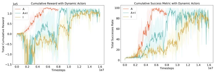
5Figure 2: The figure reports the mean cumulative reward and success rate for the three variants:
A, A + I and I on the Dynamic Navigation task [20]. The plots indicate that the A and A + I learn
the navigation task successfully whereas the state-representation I learns the task slowly as observed
by the performance improvement after 12M time steps of training. Shaded region corresponds to the
minimum and maximum values across 3 different seeds.
then queried at each time step from the simulator, which in real-world can be accessible from the
perception and GPS subsystems. The agent steps through the simulator at every time step collecting
on-policy rollouts that determine the updates to the policy and critic networks. The episode is
terminated upon a collision, lane invasion, or traffic light infraction, or is deemed as a success if the
agent reaches within distance d m of the destination. This procedure repeats until the policy function
approximator converges to the optimal policy. The actor and critic networks consist of a standard
2-layer feedforward network. All the networks are trained with a ReLU non-linearity and optimized
using stochastic gradient descent with the Adam optimizer. The overall architecture of our approach
is depicted in Fig. 1 and the overall algorithm is summarized in Algo. 1.
4 Experiments
To implement our proposed algorithm (Algo. 1), we build on top of stable-baselines implementation
[28] and train our entire setup in the CARLA simulator [20]. The training is performed on the
Dynamic Navigation task of the original CARLA benchmark [20] and it is evaluated across all tasks
of the same benchmark. Since this benchmark considers an episode to be successful regardless of
any collisions or other infractions, we extend our evaluation to the recent NoCrash benchmark [16]
that proposes dynamic actor tasks that count collision as infractions. We then conduct a thorough
infraction analysis that helps us analyze the different types of episode terminations and their relative
proportions in order to understand the behavior and robustness of the policy learned by our agent.
4.1 Baselines
For comparing our method with the prior work, we choose modular, imitation learning and reinforce-
ment learning baselines that solve the goal-directed navigation task and report results on the original
CARLA [20] and NoCrash [16] benchmarks. The modular baselines include MP [20], CAL [60] and
AT, which is the automatic control agent available within CARLA distribution. IL [20], CIL [15],
CILRS [16] and LBC [13] form our imitation learning baselines whereas on the reinforcement learning
end we choose RL [20], CIRL [40] and IA [69]. We point readers to refer the Appendix for a brief
summary of each of our chosen baselines. Although all of the above baselines use forward-facing
RGB image and high-level navigational command as inputs, we recognize the differences in our
inputs and presume that the current state-of-the-art perception systems are capable of predicting the
low-dimensional representations or semantic labels with reasonable accuracy. Additionally, we do
not consider the pedestrian actors in our setup owing to the limitations of CARLA 0.9.6 version.
5 Results
Comparing the training stability across our three variants (A, A + I, or I) as defined in Sec. 3, we
observe from Fig. 2 that the variant A that explicitly uses affordances, performs the best as it is
6NoCrash Benchmark (% Success Episodes)
Task Training Conditions (Town 01)
CIL CAL CILRS LBC IA AT Ours (A) Ours (A+I) Ours (I)
Empty 79 ± 1 81 ± 1 87 ± 1 97 ± 1 100 100 ± 0 100 ± 0 100 ± 0 94 ± 10
Regular 60 ± 1 73 ± 2 83 ± 0 93 ± 1 96 99 ± 1 98 ± 2 90 ± 2 90 ± 4
Dense 21 ± 2 42 ± 1 42 ± 2 71 ± 5 70 86 ± 3 95 ± 2 94 ± 4 89 ± 4
Task Testing Conditions (Town 02)
CIL CAL CILRS LBC IA AT Ours (A) Ours (A+I) Ours (I)
Empty 48 ± 3 36 ± 6 51 ± 1 100 ± 0 99 100 ± 0 100 ± 0 100 ± 0 98 ± 3
Regular 27 ± 1 26 ± 2 44 ± 5 94 ± 3 87 99 ± 1 98 ± 1 96 ± 2 96 ± 2
Dense 10 ± 2 9±1 38 ± 2 51 ± 3 42 60 ± 3 91 ± 1 89 ± 2 79 ± 3
Table 1: Quantitative comparison with the baselines on the NoCrash benchmark [16]. The table
reports the percentage (%) of successfully completed episodes for each task in the training and testing
town. Higher is better. The baselines include CIL [15], CAL [60], CILRS [16], LBC [13], IA [69]
and CARLA built-in autopilot control (AT) compared with our PPO method. Results denote average
of 3 seeds across 5 trials. Bold values correspond to the best mean success rate.
stably able to learn the dynamic navigation task on the original CARLA benchmark [20] within 6M
timesteps. We also see that the variants I and A + I, take almost twice the timesteps (12M) to reach
similar performance. I is slower compared with the other two variants, which makes us empirically
believe that it requires more samples to learn the dynamic obstacle affordance when compared with
the latter that explicitly encode it.
Considering our input representation includes low-dimensional representations or latent features of
semantically segmented images, we compare and present results only on training weather conditions
from all the baselines. For evaluation, we pick the best performing model from each seed based on
the cumulative reward it collects at the time of validation and report results averaged over 3 seeds and
5 different evaluations of the benchmarks.
5.1 Evaluation on the Original CARLA Benchmark
On the original CARLA benchmark [20], we note that both the variants A and A + I (Table. 3)
achieve a perfect success percentage on all the driving tasks in both Town 01 and Town 02, whereas
the variant I achieves near-perfect success percentage. The driving policy learned by our agent
demonstrates stopping in front of other actors or traffic lights in red-state while perfectly navigating
through the town and around intersections. Further, for all the variants, our results also demonstrate
that on the most difficult driving task of Dynamic Navigation, we achieve a significant improvement
in the success rate performance on both towns when compared with our baselines such as MP [20], IL
[20], RL [20], CIL [15], CIRL [40] and CAL [60]. For CILRS [16], the improvement is significant for
Town 02 and moderate for Town 01. We also note that our method reports comparable performance to
the recent works of LBC [13] and IA [69] on some of the tasks.
5.2 Evaluation on the NoCrash Benchmark
On the NoCrash benchmark [16], our quantitative results (Table 1) again demonstrate that our driving
agent learns the optimal control almost perfectly across different levels of traffic and town conditions.
The variant A outperforms the variant A + I which outperforms variant I. This difference can be
attributed to the low-dimensionality of the state representation A. Moreover, we also note that the
success rate performance achieved by our agent is significantly higher than all the prior modular and
imitation learning baselines such as CIL [15], CAL [60], CILRS [16], LBC [13] and IA [69]. The
AT baseline, which refers to the autopilot control that is shipped with the CARLA binaries, uses a
hand-engineered approach to determine the optimal control. We observe that even on the hardest
task of Dense traffic, our method using all three variants significantly outperforms even the most
engineered approach to urban driving. For a qualitative analysis, we publish a video2 of our agent
successfully driving on the dynamic navigation task. We presume that our near-perfect results can
be accounted for our simpler choice of input representation. Thus for a fair comparison, our future
direction is to move towards high-dimensional RGB images. Nevertheless, a notable difference
between the baseline methods and our method is that they use strong supervision signals, unlike our
2
https://www.youtube.com/watch?v=AwbJSPtKHkY
7Infraction Analysis on NoCrash Benchmark (% Episodes)
Task Metric Training Conditions (Town 01) Testing Conditions (Town 02)
CIL CAL CILRS Ours (A) CIL CAL CILRS Ours (A)
Success 79.00 84.00 96.33 100.00 41.67 48.67 72.33 100.00
Col. Vehicles 0.00 0.00 0.00 0.00 0.00 0.00 0.00 0.00
Empty
Col. Other 11.00 9.00 1.33 0.00 51.00 45.33 20.00 0.00
Timeout 10.00 7.00 2.33 0.00 7.33 6.00 7.67 0.00
Success 61.50 57.00 87.33 98.40 22.00 27.67 49.00 98.16
Col. Vehicles 16.00 26.00 4.00 0.27 34.67 30.00 12.67 0.00
Regular
Col. Other 16.50 14.00 5.67 0.53 37.33 36.33 28.00 0.92
Timeout 6.00 3.00 3.00 0.80 6.00 6.00 10.33 0.92
Success 22.00 16.00 41.66 95.38 7.33 10.67 21.00 91.20
Col. Vehicles 49.50 57.00 20.67 0.62 55.67 46.33 35.00 3.73
Dense
Col. Other 25.00 24.00 34.67 1.23 34.33 35.33 35.00 1.87
Timeout 3.50 3.00 3.00 2.77 2.67 7.67 9.00 3.20
Table 2: Quantitative analysis of episode termination causes and comparison with the baselines on
the NoCrash benchmark [16]. The table reports the percentage (%) of episodes with their termination
causes for each task in the training and testing town. The columns for a single method/task/condition
should add up to 1. Bold values correspond to the best performance for each termination condition.
Results denote average of 3 seeds across 5 trials.
method that learns the optimal policy from scratch based on trial-and-error learning. These supervised
signals, often expensive to collect, do not always capture the distribution of scenarios entirely. In
contrast, we show that our results demonstrate the prospects of utilizing reinforcement learning to
learn complex urban driving behaviors.
5.3 Infraction Analysis
To analyze the failure cases of our agent, we also perform an infraction analysis on variant A that
reports the percentage of episodes for each termination condition and driving task on the NoCrash
benchmark [16]. We then compare this analysis with few of our baselines like CIL [15], CAL [60]
and CILRS [16] that perform end-to-end imitation learning or take a modular approach to predicting
low-dimensional affordances like ours. We incorporate the baseline infraction metrics from the CILRS
work [16]. We observe from this analysis (Table 2) that our agent significantly outperforms all the
other baselines across all traffic and town conditions. Further, we note that our agent in the Empty
town task achieves a perfect success percentage across both Town 01 and Town 02 without facing
any infractions. Additionally, on the Regular and Dense traffic tasks, we notice that our approach
reduces the number of collision and timeout infractions by at least an order of magnitude across both
the towns. Therefore, our results indicate that the policy learned by our agents using reinforcement
learning is robust to variability in both traffic and town conditions.
6 Conclusion
In this work, we present an approach to learn urban driving tasks that commonly subtasks such as
lane-following, driving around intersections and handling numerous interactions between dynamic
actors, and traffic signs and signals. We formulate a reinforcement learning-based approach primarily
based around three different variants that use waypoints and low-dimensional visual affordances. We
demonstrate that using such low-dimensional representations makes the planning and control problem
easier as we can learn stable and robust policies demonstrated by our results with state representation
A. Further, we also observe that as we move towards learning these representations inherently
using convolutional encoders, the performance and robustness of our learned policy decreases which
requires more training samples to learn the optimal representations, as evident from Fig. 2 and
the results presented in Sec. 5. We also note that our method when trained from scratch achieves
comparable or better performance than most baselines methods that often require expert supervision
to learn control policies. We also show that our agent learned with variant A reports a significantly
lower number of infractions that are at least an order of magnitude less than the prior works on the
same tasks. Thus, our work shows the strong potential of using reinforcement learning for learning
autonomous driving behaviours and we hope it inspires more research in the future.
8References
[1] Pieter Abbeel, Adam Coates, and Andrew Y Ng. Autonomous helicopter aerobatics through apprenticeship
learning. The International Journal of Robotics Research, 29(13):1608–1639, 2010.
[2] Tanmay Agarwal, Hitesh Arora, Tanvir Parhar, Shuby Deshpande, and Jeff Schneider. Learning to drive
using waypoints. In Workshop on ‘Machine Learning for Autonomous Driving’ at Conference on Neural
Information Processing Systems, 2019.
[3] Ilge Akkaya, Marcin Andrychowicz, Maciek Chociej, Mateusz Litwin, Bob McGrew, Arthur Petron, Alex
Paino, Matthias Plappert, Glenn Powell, Raphael Ribas, et al. Solving rubik’s cube with a robot hand.
arXiv preprint arXiv:1910.07113, 2019.
[4] Eduardo Arnold, Omar Y Al-Jarrah, Mehrdad Dianati, Saber Fallah, David Oxtoby, and Alex Mouzakitis.
A survey on 3d object detection methods for autonomous driving applications. IEEE Transactions on
Intelligent Transportation Systems, 20(10):3782–3795, 2019.
[5] Karl Johan Åström and Tore Hägglund. PID controllers: theory, design, and tuning, volume 2. Instrument
society of America Research Triangle Park, NC, 1995.
[6] Claudine Badue, Rânik Guidolini, Raphael Vivacqua Carneiro, Pedro Azevedo, Vinicius Brito Cardoso,
Avelino Forechi, Luan Jesus, Rodrigo Berriel, Thiago Paixao, Filipe Mutz, et al. Self-driving cars: A
survey. arXiv preprint arXiv:1901.04407, 2019.
[7] Mayank Bansal, Alex Krizhevsky, and Abhijit Ogale. Chauffeurnet: Learning to drive by imitating the
best and synthesizing the worst. arXiv preprint arXiv:1812.03079, 2018.
[8] Mariusz Bojarski, Davide Del Testa, Daniel Dworakowski, Bernhard Firner, Beat Flepp, Prasoon Goyal,
Lawrence D Jackel, Mathew Monfort, Urs Muller, Jiakai Zhang, et al. End to end learning for self-driving
cars. arXiv preprint arXiv:1604.07316, 2016.
[9] Mariusz Bojarski, Philip Yeres, Anna Choromanska, Krzysztof Choromanski, Bernhard Firner, Lawrence
Jackel, and Urs Muller. Explaining how a deep neural network trained with end-to-end learning steers a
car. arXiv preprint arXiv:1704.07911, 2017.
[10] Michael Brady, John M Hollerbach, Timothy L Johnson, Tomás Lozano-Pérez, Matthew T Mason, Daniel G
Bobrow, Patrick Henry Winston, and Randall Davis. Robot motion: Planning and control. MIT press,
1982.
[11] Guillaume Bresson, Zayed Alsayed, Li Yu, and Sébastien Glaser. Simultaneous localization and mapping:
A survey of current trends in autonomous driving. IEEE Transactions on Intelligent Vehicles, 2(3):194–220,
2017.
[12] Mark Campbell, Magnus Egerstedt, Jonathan P How, and Richard M Murray. Autonomous driving in
urban environments: approaches, lessons and challenges. Philosophical Transactions of the Royal Society
A: Mathematical, Physical and Engineering Sciences, 368(1928):4649–4672, 2010.
[13] Dian Chen, Brady Zhou, Vladlen Koltun, and Philipp Krähenbühl. Learning by cheating. In Conference
on Robot Learning, pages 66–75, 2020.
[14] Lu Chi and Yadong Mu. Deep steering: Learning end-to-end driving model from spatial and temporal
visual cues. arXiv preprint arXiv:1708.03798, 2017.
[15] Felipe Codevilla, Matthias Miiller, Antonio López, Vladlen Koltun, and Alexey Dosovitskiy. End-to-end
driving via conditional imitation learning. In 2018 IEEE International Conference on Robotics and
Automation (ICRA), pages 1–9. IEEE, 2018.
[16] Felipe Codevilla, Eder Santana, Antonio M López, and Adrien Gaidon. Exploring the limitations of
behavior cloning for autonomous driving. In Proceedings of the IEEE International Conference on
Computer Vision, pages 9329–9338, 2019.
[17] Will Dabney, Georg Ostrovski, David Silver, and Rémi Munos. Implicit quantile networks for distributional
reinforcement learning. arXiv preprint arXiv:1806.06923, 2018.
[18] Guilherme N DeSouza and Avinash C Kak. Vision for mobile robot navigation: A survey. IEEE
transactions on pattern analysis and machine intelligence, 24(2):237–267, 2002.
[19] Nemanja Djuric, Vladan Radosavljevic, Henggang Cui, Thi Nguyen, Fang-Chieh Chou, Tsung-Han Lin,
and Jeff Schneider. Motion prediction of traffic actors for autonomous driving using deep convolutional
networks. arXiv preprint arXiv:1808.05819, 2, 2018.
[20] Alexey Dosovitskiy, Germán Ros, Felipe Codevilla, Antonio López, and Vladlen Koltun. Carla: An open
urban driving simulator. In CoRL, 2017.
[21] Roy Featherstone and David Orin. Robot dynamics: equations and algorithms. In Proceedings 2000
ICRA. Millennium Conference. IEEE International Conference on Robotics and Automation. Symposia
Proceedings (Cat. No. 00CH37065), volume 1, pages 826–834. IEEE, 2000.
9[22] David A Forsyth and Jean Ponce. Computer vision: a modern approach. Prentice Hall Professional
Technical Reference, 2002.
[23] Andreas Geiger, Philip Lenz, Christoph Stiller, and Raquel Urtasun. Vision meets robotics: The kitti
dataset. The International Journal of Robotics Research, 32(11):1231–1237, 2013.
[24] Shixiang Gu, Ethan Holly, Timothy Lillicrap, and Sergey Levine. Deep reinforcement learning for robotic
manipulation with asynchronous off-policy updates. In 2017 IEEE international conference on robotics
and automation (ICRA), pages 3389–3396. IEEE, 2017.
[25] P. E. Hart, N. J. Nilsson, and B. Raphael. A formal basis for the heuristic determination of minimum cost
paths. IEEE Transactions on Systems Science and Cybernetics, 4(2):100–107, 1968.
[26] Kaiming He, Xiangyu Zhang, Shaoqing Ren, and Jian Sun. Deep residual learning for image recognition.
In Proceedings of the IEEE conference on computer vision and pattern recognition, pages 770–778, 2016.
[27] Matteo Hessel, Joseph Modayil, Hado Van Hasselt, Tom Schaul, Georg Ostrovski, Will Dabney, Dan
Horgan, Bilal Piot, Mohammad Azar, and David Silver. Rainbow: Combining improvements in deep
reinforcement learning. In Thirty-Second AAAI Conference on Artificial Intelligence, 2018.
[28] Ashley Hill, Antonin Raffin, Maximilian Ernestus, Adam Gleave, Anssi Kanervisto, Rene Traore, Prafulla
Dhariwal, Christopher Hesse, Oleg Klimov, Alex Nichol, Matthias Plappert, Alec Radford, John Schulman,
Szymon Sidor, and Yuhuai Wu. Stable baselines. https://github.com/hill-a/stable-baselines,
2018.
[29] Dan Horgan, John Quan, David Budden, Gabriel Barth-Maron, Matteo Hessel, Hado Van Hasselt, and
David Silver. Distributed prioritized experience replay. arXiv preprint arXiv:1803.00933, 2018.
[30] Takeo Kanade, Chuck Thorpe, and William Whittaker. Autonomous land vehicle project at cmu. In
Proceedings of the 1986 ACM fourteenth annual conference on Computer science, pages 71–80, 1986.
[31] Alex Kendall, Jeffrey Hawke, David Janz, Przemyslaw Mazur, Daniele Reda, John-Mark Allen, Vinh-Dieu
Lam, Alex Bewley, and Amar Shah. Learning to drive in a day. In 2019 International Conference on
Robotics and Automation (ICRA), pages 8248–8254. IEEE, 2019.
[32] Qadeer Khan, Torsten Schön, and Patrick Wenzel. Latent space reinforcement learning for steering angle
prediction. arXiv preprint arXiv:1902.03765, 2019.
[33] B Ravi Kiran, Ibrahim Sobh, Victor Talpaert, Patrick Mannion, Ahmad A Al Sallab, Senthil Yogamani,
and Patrick Pérez. Deep reinforcement learning for autonomous driving: A survey. arXiv preprint
arXiv:2002.00444, 2020.
[34] Alex Krizhevsky, Ilya Sutskever, and Geoffrey E Hinton. Imagenet classification with deep convolutional
neural networks. In Advances in neural information processing systems, pages 1097–1105, 2012.
[35] Sampo Kuutti, Saber Fallah, Konstantinos Katsaros, Mehrdad Dianati, Francis Mccullough, and Alexandros
Mouzakitis. A survey of the state-of-the-art localization techniques and their potentials for autonomous
vehicle applications. IEEE Internet of Things Journal, 5(2):829–846, 2018.
[36] Jean-Paul Laumond et al. Robot motion planning and control, volume 229. Springer, 1998.
[37] Yann LeCun, Yoshua Bengio, and Geoffrey Hinton. Deep learning. nature, 521(7553):436–444, 2015.
[38] Stéphanie Lefèvre, Dizan Vasquez, and Christian Laugier. A survey on motion prediction and risk
assessment for intelligent vehicles. ROBOMECH journal, 1(1):1–14, 2014.
[39] Jesse Levinson, Jake Askeland, Jan Becker, Jennifer Dolson, David Held, Soeren Kammel, J Zico Kolter,
Dirk Langer, Oliver Pink, Vaughan Pratt, et al. Towards fully autonomous driving: Systems and algorithms.
In 2011 IEEE Intelligent Vehicles Symposium (IV), pages 163–168. IEEE, 2011.
[40] Xiaodan Liang, Tairui Wang, Luona Yang, and Eric P. Xing. Cirl: Controllable imitative reinforcement
learning for vision-based self-driving. In ECCV, 2018.
[41] Timothy P Lillicrap, Jonathan J Hunt, Alexander Pritzel, Nicolas Heess, Tom Erez, Yuval Tassa, David
Silver, and Daan Wierstra. Continuous control with deep reinforcement learning. arXiv preprint
arXiv:1509.02971, 2015.
[42] Volodymyr Mnih, Adria Puigdomenech Badia, Mehdi Mirza, Alex Graves, Timothy Lillicrap, Tim Harley,
David Silver, and Koray Kavukcuoglu. Asynchronous methods for deep reinforcement learning. In
International conference on machine learning, pages 1928–1937, 2016.
[43] Volodymyr Mnih, Koray Kavukcuoglu, David Silver, Alex Graves, Ioannis Antonoglou, Daan Wierstra,
and Martin Riedmiller. Playing atari with deep reinforcement learning. arXiv preprint arXiv:1312.5602,
2013.
[44] Volodymyr Mnih, Koray Kavukcuoglu, David Silver, Andrei A Rusu, Joel Veness, Marc G Bellemare,
Alex Graves, Martin Riedmiller, Andreas K Fidjeland, Georg Ostrovski, et al. Human-level control through
deep reinforcement learning. nature, 518(7540):529–533, 2015.
10[45] Michael Montemerlo, Jan Becker, Suhrid Bhat, Hendrik Dahlkamp, Dmitri Dolgov, Scott Ettinger, Dirk
Haehnel, Tim Hilden, Gabe Hoffmann, Burkhard Huhnke, et al. Junior: The stanford entry in the urban
challenge. Journal of field Robotics, 25(9):569–597, 2008.
[46] Sajjad Mozaffari, Omar Y Al-Jarrah, Mehrdad Dianati, Paul Jennings, and Alexandros Mouzakitis. Deep
learning-based vehicle behaviour prediction for autonomous driving applications: A review. arXiv preprint
arXiv:1912.11676, 2019.
[47] Urs Muller, Jan Ben, Eric Cosatto, Beat Flepp, and Yann L Cun. Off-road obstacle avoidance through
end-to-end learning. In Advances in neural information processing systems, pages 739–746, 2006.
[48] Farzeen Munir, Shoaib Azam, Muhammad Ishfaq Hussain, Ahmed Muqeem Sheri, and Moongu Jeon.
Autonomous vehicle: The architecture aspect of self driving car. In Proceedings of the 2018 International
Conference on Sensors, Signal and Image Processing, pages 1–5, 2018.
[49] The Mercury News. Google self-driving car brakes for wheelchair lady chasing duck with broom, 2016.
[50] Ryosuke Okuda, Yuki Kajiwara, and Kazuaki Terashima. A survey of technical trend of adas and
autonomous driving. In Technical Papers of 2014 International Symposium on VLSI Design, Automation
and Test, pages 1–4. IEEE, 2014.
[51] Brian Paden, Michal Čáp, Sze Zheng Yong, Dmitry Yershov, and Emilio Frazzoli. A survey of motion
planning and control techniques for self-driving urban vehicles. IEEE Transactions on intelligent vehicles,
1(1):33–55, 2016.
[52] Yunpeng Pan, Ching-An Cheng, Kamil Saigol, Keuntaek Lee, Xinyan Yan, Evangelos Theodorou, and
Byron Boots. Agile off-road autonomous driving using end-to-end deep imitation learning. arXiv preprint
arXiv:1709.07174, 2, 2017.
[53] Anna Petrovskaya and Sebastian Thrun. Model based vehicle detection and tracking for autonomous urban
driving. Autonomous Robots, 26(2-3):123–139, 2009.
[54] Dean A Pomerleau. Alvinn: An autonomous land vehicle in a neural network. In Advances in neural
information processing systems, pages 305–313, 1989.
[55] Rajesh Rajamani. Vehicle dynamics and control. Springer Science & Business Media, 2011.
[56] Nathan D Ratliff, J Andrew Bagnell, and Martin A Zinkevich. Maximum margin planning. In Proceedings
of the 23rd international conference on Machine learning, pages 729–736, 2006.
[57] Nicholas Rhinehart, Rowan McAllister, and Sergey Levine. Deep imitative models for flexible inference,
planning, and control. arXiv preprint arXiv:1810.06544, 2018.
[58] Daniel E Rivera, Manfred Morari, and Sigurd Skogestad. Internal model control: Pid controller design.
Industrial & engineering chemistry process design and development, 25(1):252–265, 1986.
[59] Stéphane Ross, Geoffrey Gordon, and Drew Bagnell. A reduction of imitation learning and structured
prediction to no-regret online learning. In Proceedings of the fourteenth international conference on
artificial intelligence and statistics, pages 627–635, 2011.
[60] Axel Sauer, Nikolay Savinov, and Andreas Geiger. Conditional affordance learning for driving in urban
environments. arXiv preprint arXiv:1806.06498, 2018.
[61] Robert J Schalkoff. Digital image processing and computer vision, volume 286. Wiley New York, 1989.
[62] John Schulman, Filip Wolski, Prafulla Dhariwal, Alec Radford, and Oleg Klimov. Proximal policy
optimization algorithms. arXiv preprint arXiv:1707.06347, 2017.
[63] Wilko Schwarting, Javier Alonso-Mora, and Daniela Rus. Planning and decision-making for autonomous
vehicles. Annual Review of Control, Robotics, and Autonomous Systems, 2018.
[64] David Silver, J Andrew Bagnell, and Anthony Stentz. Learning from demonstration for autonomous
navigation in complex unstructured terrain. The International Journal of Robotics Research, 29(12):1565–
1592, 2010.
[65] David Silver, Aja Huang, Chris J Maddison, Arthur Guez, Laurent Sifre, George Van Den Driessche, Julian
Schrittwieser, Ioannis Antonoglou, Veda Panneershelvam, Marc Lanctot, et al. Mastering the game of go
with deep neural networks and tree search. nature, 529(7587):484–489, 2016.
[66] David Silver, Thomas Hubert, Julian Schrittwieser, Ioannis Antonoglou, Matthew Lai, Arthur Guez, Marc
Lanctot, Laurent Sifre, Dharshan Kumaran, Thore Graepel, et al. Mastering chess and shogi by self-play
with a general reinforcement learning algorithm. arXiv preprint arXiv:1712.01815, 2017.
[67] Santokh Singh. Critical reasons for crashes investigated in the national motor vehicle crash causation
survey. Technical report, 2018.
[68] Umar Syed and Robert E Schapire. A game-theoretic approach to apprenticeship learning. In Advances in
neural information processing systems, pages 1449–1456, 2008.
11[69] Marin Toromanoff, Emilie Wirbel, and Fabien Moutarde. End-to-end model-free reinforcement learning
for urban driving using implicit affordances. In Proceedings of the IEEE/CVF Conference on Computer
Vision and Pattern Recognition, pages 7153–7162, 2020.
[70] Richard S Wallace, Anthony Stentz, Charles E Thorpe, Hans P Moravec, William Whittaker, and Takeo
Kanade. First results in robot road-following. In IJCAI, pages 1089–1095. Citeseer, 1985.
[71] Bernhard Wymann, Eric Espié, Christophe Guionneau, Christos Dimitrakakis, Rémi Coulom, and Andrew
Sumner. Torcs, the open racing car simulator. Software available at http://torcs. sourceforge. net, 4(6):2,
2000.
[72] Huazhe Xu, Yang Gao, Fisher Yu, and Trevor Darrell. End-to-end learning of driving models from large-
scale video datasets. In Proceedings of the IEEE conference on computer vision and pattern recognition,
pages 2174–2182, 2017.
[73] Zhengyuan Yang, Yixuan Zhang, Jerry Yu, Junjie Cai, and Jiebo Luo. End-to-end multi-modal multi-task
vehicle control for self-driving cars with visual perceptions. In 2018 24th International Conference on
Pattern Recognition (ICPR), pages 2289–2294. IEEE, 2018.
[74] Ekim Yurtsever, Jacob Lambert, Alexander Carballo, and Kazuya Takeda. A survey of autonomous driving:
Common practices and emerging technologies. IEEE Access, 8:58443–58469, 2020.
[75] Fangyi Zhang, Jürgen Leitner, Michael Milford, Ben Upcroft, and Peter Corke. Towards vision-based deep
reinforcement learning for robotic motion control. arXiv preprint arXiv:1511.03791, 2015.
[76] Jiakai Zhang and Kyunghyun Cho. Query-efficient imitation learning for end-to-end autonomous driving.
arXiv preprint arXiv:1605.06450, 2016.
12Appendix
Algorithm
Algorithm 1 Learning to Drive via Model-Free RL on Learned Representations
1: Input: initial policy parameters θ0 , initial value function parameters φ0 , pretrained auto-encoder
parameters β0 ,
2: for k = 0, 1, 2, . . . do
3: Collect trajectories Dk = {τi } by running policy πθk in the environment.
4: Compute rewards-to-go R̂t .
5: Compute advantage estimates, Ât based on the current value function Vφk .
6: Update the policy by maximizing the PPO-Clip objective.
T
1 X X
θk+1 = arg max min r(θ)Aπθk (st , at ), clip r(θ), 1−, 1+ Aπθk (st , at )
θ |Dk | T
τ ∈Dk
t=0
7: Fit value function by regression on mean-squared error.
T 2
1 X X
φk+1 = arg min Vφ (st ) − R̂t
φ |Dk | T
τ ∈Dk
t=0
8: Every fixed n steps, finetune the autoencoder based on cross-entropy loss.
X X
βk+1 = arg min (−tc (p) log oc (p))
β
p∈SSimage c∈C
9: end for
Summary of Baselines
We compare our work with the following baselines that solve the goal-directed navigation task using
an either modular approach, end-to-end imitation learning, or reinforcement learning. Since most of
the works do not have open-source implementations available or report results on the older versions
of CARLA, we report the numbers directly from their work.
• CARLA MP, IL & RL [20]: These baselines, proposed in the original CARLA work
[20] suggest three different approaches to the autonomous driving task. The modular
pipeline (MP) uses a vision-based module, a rule-based planner, and a classical controller.
The imitation learning (IL) one learns a deep network that maps sensory input to driving
commands whereas the reinforcement learning (RL) baseline does end-to-end RL using the
A3C algorithm [42].
• AT: This baseline refers to the CARLA built-in autopilot control that uses a hand-engineered
approach to determine optimal control.
• CIL [15]: This work proposes a conditional imitation learning pipeline that learns a driving
policy from expert demonstrations of low-level control inputs, conditioned on the high-level
navigational command.
• CIRL [40]: This work proposes to use a pre-trained imitation learned policy to carry-out
off-policy reinforcement learning using the DDPG algorithm [41].
• CAL [60]: This baseline proposes to learn a separate visual encoder that predicts low-
dimensional representations, also known as affordances, that are essential for urban driving.
These representations are then fused with classical controllers.
• CILRS [16]: This work builds on top of CIL [15] to propose a robust behavior cloning
pipeline that generalizes well to complex driving scenarios. The method suggests learning
13a ResNet architecture [26] that predicts the desired control as well as the agent’s speed to
learn speed-related features from visual cues.
• LBC [13]: This work decouples the sensorimotor learning task into two, learning to see and
learning to act. In the first step, a privileged agent is learned that has access to the simulator
states and learns to act. The second step involves learning to see that learns an agent based
on supervision provided by the privileged agent.
• IA [69]: This work proposes to learn a ResNet encoder [26] that predicts the implicit
affordances and uses its output features to learn a separate policy network optimized using
DQN algorithm [43].
Evaluation on the Original CARLA Benchmark
On the original CARLA benchmark [20], we note that both the variants A and A + I (Table. 3)
achieve a perfect success percentage on all the driving tasks in both Town 01 and Town 02, whereas
the variant I achieves near-perfect success percentage.
Original CARLA Benchmark (% Success Episodes)
Task Training Conditions (Town 01)
MP IL RL CIL CIRL CAL CILRS LBC IA Ours (A) Ours (A+I) Ours (I)
Straight 98 95 89 98 98 100 96 100 100 100 ± 0 100 ± 0 99 ± 2
One Turn 82 89 34 89 97 97 92 100 100 100 ± 0 100 ± 0 100 ± 0
Navigation 80 86 14 86 93 92 95 100 100 100 ± 0 100 ± 0 96 ± 7
Dyn. Navigation 77 83 7 83 82 83 92 100 100 100 ± 0 100 ± 0 95 ± 7
Task Testing Conditions (Town 02)
MP IL RL CIL CIRL CAL CILRS LBC IA Ours (A) Ours (A+I) Ours (I)
Straight 92 97 74 97 100 93 96 100 100 100 ± 0 100 ± 0 100 ± 0
One Turn 61 59 12 59 71 82 84 100 100 100 ± 0 100 ± 0 97 ± 2
Navigation 24 40 3 40 53 70 69 98 100 100 ± 0 99 ± 1 100 ± 0
Dyn. Navigation 24 38 2 38 41 64 66 99 98 100 ± 0 100 ± 0 99 ± 1
Table 3: Quantitative comparison with the baselines that solve the four goal-directed navigation
tasks using modular, imitation learning or reinforcement learning approaches on the original CARLA
benchmark [20]. The table reports the percentage (%) of successfully completed episodes for each
task in the training (Town 01) and testing town (Town 02). Higher is better. The baselines include MP
[20], IL [20], RL [20], CIL [15], CIRL [40], CAL [60], CILRS [16], LBC [13] and IA [69] compared
with our PPO method. Results denote average of 3 seeds across 5 trials. Bold values correspond to
the best mean success rate.
Hyperparameters
CARLA Environment
In this subsection, we detail all the parameters we use for our experiments with the CARLA simulator
[20]. The list mentioned below covers all the parameters to the best of our knowledge, except those
that are set to default values in the simulator.
• Camera top-down co-ordinates: (x = 13.0, y = 0.0, z = 18.0, pitch = 270◦ )
• Camera front-facing co-ordinates: (x = 2.0, y = 0.0, z = 1.4, pitch = 0◦ )
• Camera image resolution: (x = 128, y = 128)
• Camera field-of-view = 90
• Server frame-rate = 10f ps
• Maximum target-speed = 20km/h
• PID parameters: (KP = 0.1, KD = 0.0005, KI = 0.4, dt = 1/10.0)
• Waypoint resolution (wd ) = 2m
• Number of next waypoints (n) = 5
• Maximum time steps (m) = 10000
• Success distance from goal (d) = 10m
14Algorithm Hyperparameters
In this subsection, we detail all the algorithm hyper-parameters used for the experiments and results
reported in Sec. 5. The list mentioned below covers all the parameters to the best of our knowledge,
except those that are set to default values as defined in the stable baselines documentation [28].
• Total training time steps = 16M
• N-steps = 10000
• Number of epochs = 10
• Number of minibatches = 20
• Clip parameter = 0.1
• Speed-based reward coefficient (α) = 1
• Distance-based penalty from optimal trajectory (β) = 1
• Infraction penalty speed-based coefficient (γ) = 250
• Infraction penalty constant coefficient (δ) = 250
• Learning rate = 0.0002
• Validation interval = 40K
• Number of dynamic actors at training time = U(70, 150), where U refers to uniform distri-
bution.
• Image frame-stack fed to autoencoder (k) = 3
• Dynamic obstacle proximity threshold (dprox ) = 15m
• Traffic light proximity threshold (tprox ) = 15m
• Minimum threshold distance for traffic light detection = 6m
• Random seeds = 3
• Number of benchmark evaluations = 5
15You can also read