Path planning and smoothing of mobile robot based on improved artificial fish swarm algorithm - Nature
←
→
Page content transcription
If your browser does not render page correctly, please read the page content below
www.nature.com/scientificreports
OPEN Path planning and smoothing
of mobile robot based on improved
artificial fish swarm algorithm
Fei‑Fei Li, Yun Du & Ke‑Jin Jia*
An algorithm that integrates the improved artificial fish swarm algorithm with continuous segmented
Bézier curves is proposed, aiming at the path planning and smoothing of mobile robots. On the one
hand, to overcome the low accuracy problems, more inflection points and relatively long planning
paths in the traditional artificial fish swarm algorithm for path planning, feasible solutions and a range
of step sizes are introduced based on Dijkstra’s algorithm. To solve the problems of poor convergence
and degradation that hinder the algorithm’s ability to find the best in the later stage, a dynamic
feedback horizon and an adaptive step size are introduced. On the other hand, to ensure that the
planned paths are continuous in both orientation and curvature, the Bessel curve theory is introduced
to smooth the planned paths. This is demonstrated through a simulation that shows the improved
artificial fish swarm algorithm achieving 100% planning accuracy, while ensuring the shortest average
path in the same grid environment. Additionally, the smoothed path is continuous in both orientation
and curvature, which satisfies the kinematic characteristics of the mobile robot.
Path planning has become a hot topic as mobile robots are widely used in industrial, service and medical indus-
tries, among others. Path planning is an important area of research in mobile robotics, where the goal is to plan
a collision-free route from a starting point to a target point. The path planning problem can also be formulated
as an optimization problem subject to several constraints and performance criteria1 (e.g., shortest distance,
feasibility of the path, whether kinematic constraints are satisfied). To date, a large number of algorithms have
been available for path planning of mobile robots, such as the ant colony algorithm2, particle swarm algorithm3,
A* algorithm4, artificial potential field algorithm5, genetic algorithm6, neural network algorithm7 and rapid
exploration random tree (RRT)8. Among them, the ant colony algorithm is relatively sensitive to the initial
parameters, and different parameters reduce the algorithm’s searchability. Some individual ants become lost in
the search process, and a large number of incomplete paths appear. The particle swarm algorithm requires a large
number of samples to approximate the posterior probability of the system, and the validity and diversity of the
samples cannot be guaranteed in the resampling stage, which leads to the depletion of the samples. Thus, the
algorithm is computationally intensive. Planning paths is tedious for the A* algorithm, and the algorithm often
generates a large number of invalid search paths. The artificial potential field method is prone to local optimal-
ity and deadlock. The genetic algorithm relies on experience for selecting relevant parameters and is prone to
being "premature." The neural network is computationally intensive and requires a large number of data models
for training. The fast exploration of randomized trees requires considerable memory due to too many nodes.
Based on the above problems, many people introduce new bionic algorithms for planning and design. The
artificial fish swarm algorithm is one of them. An artificial fish swarm is a parallel stochastic search algorithm
with advantages, such as good robustness, strong global searchability, large tolerance of parameter setting, and
insensitivity to initial v alues9, which is suitable for path planning. However, there are also some shortcomings, and
for the defects of the traditional artificial fish swarm algorithm, i n10, the parameters visual, step, δ are adjusted by
self-tuning in due time to achieve the purpose of improving the convergence accuracy. I n11, an adaptive improved
artificial fish swarm algorithm that ignores the crowding factor was proposed and applied to the path planning
of mobile robots. I n12, an improved artificial fish swarm algorithm based on the dynamic step range and field
of view range was proposed to realize the transformation of the algorithm from coarse search to fine search,
thus improving the convergence of the algorithm. I n13, a logarithmic function adaptive artificial fish swarming
algorithm (ALF-AFSA) was proposed, which uses a logarithmic function as the step range to improve the algo-
rithm’s search capability. In14, an aggregation degree factor is introduced to obtain the adaptive step range and
field of view range. Additionally, a weight evaluation factor is introduced in the fish swarm behavior to solve the
School of Electrical Engineering, Hebei University of Science and Technology, Shijiazhuang 050018, China. *email:
jwuser@126.com
Scientific Reports | (2022) 12:659 | https://doi.org/10.1038/s41598-021-04506-y 1
Vol.:(0123456789)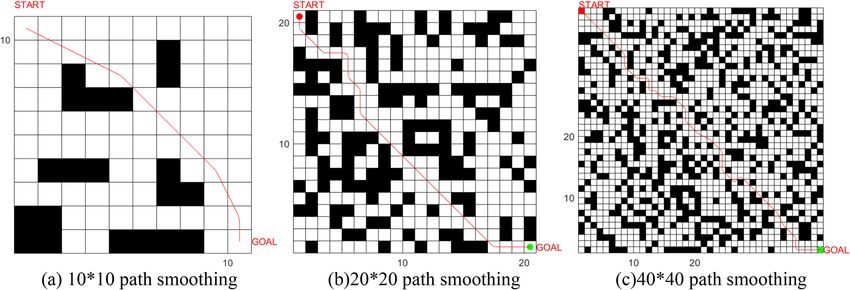
www.nature.com/scientificreports/
(a)The actual shape of the obstacle (b)The result after puffing treatment
Figure 1. Grid map environment construction.
problem that the algorithm easily falls into a local optimum and is premature. In15, four behaviors of fish swarms
were introduced with an adaptive strategy, variational strategy and hybrid strategy, and the step range and field
of view range of the hyperbolic tangent function were added to optimize the optimal finding ability and improve
the convergence speed, which was applied to solve the flow shop scheduling (FFS) problem16. The efficiency of the
algorithm was proven by experiments. Additionally, the mobile robot driving path must satisfy the continuity of
direction and curvature. I n17, the path was smoothed by combining three uniform B splines. I n18, a sequence of
planned path points was fitted using the cubic Hermit spline method, which generates monotonic curves for all
path points where curvature is discontinuous at the path points. However, many algorithms solve the smooth-
ing problem either by splicing straight and circular segments or by using spline curves without considering the
dynamical state of the mobile robot.
The above improved artificial fish swarming algorithms all successfully solve the deficiencies of AFSA in the
corresponding application areas, but some of the improved algorithms cannot reach the desired expectations
in the grid environment. In the grid environment, the traditional artificial fish swarming algorithm has two
types of movement: 4 movement directions with 4 neighborhoods and 8 movement directions with 8 neighbor-
hoods. In this paper, we propose an improved artificial fish swarm algorithm with 16 moving directions and 24
neighborhoods, which makes the artificial fish have more directional choices and wider moving range during
swimming. To avoid the phenomenon of individual crossing the barrier in the 16-Direction 24-Neighborhood
due to the relatively large step size of the artificial fish, Dijkstra’s algorithm is introduced to determine part of
the step size range of the 16-Direction 24-Neighborhood again. To overcome the problem that the global opti-
mal solution and the local optimal solution interfere with each other, the feasible solution is introduced and the
optimal path is found in the feasible solution, thus, improving the planning accuracy and ensuring the shortest
planning path. To overcome the problem that the computational volume increases due to the introduction of
Dijkstra’s algorithm, the sharing mechanism is introduced, i.e., the fish population in the same grid point can
share the obstacle information in the step length range. To ensure that the planned path is more consistent with
the kinematic characteristics of the mobile robot, the path smoothing algorithm is designed for the generated
polyline segments after the initial path points are obtained. Thus, the generated curve is a continuous function
in both orientation and curvature of the path. Finally, the feasibility and effectiveness of the algorithm are veri-
fied by simulation experiments.
Grid environment establishment. The grid graph is the most commonly used environmental modeling
method in path planning. The combined algorithm of dilation and erosion of obstacles in Fig. 1a is carried out
by morphology to extract features and reduce the complexity of the modeling environment to obtain Fig. 1b.
This paper uses the grid method to model obstacles with 0, corresponding to black squares in the grid map, 1
representing feasible areas, and corresponding to white squares in the grid map, as shown in Fig. 2.
In the grid map, each grid has a unique coordinate location corresponding to it, and the relationship between
the grid sequence number and the coordinates is as follows (1):
x = fix((i − 1)/Nx ) + 1
y = mod ((i − 1), Ny ) + 1 (1)
N = N = size(a, 1)
x y
In Eq. (1), (x, y) is the coordinate of the grid, fix() is the integral function, and mod() is the residual function.
Nx and Ny are the maximum rows and columns of the grid map, respectively, which are equal to the maximum
rows of the matrix.
In the grid map, the objective function of the optimization problem can be expressed as follows (2):
Scientific Reports | (2022) 12:659 | https://doi.org/10.1038/s41598-021-04506-y 2
Vol:.(1234567890)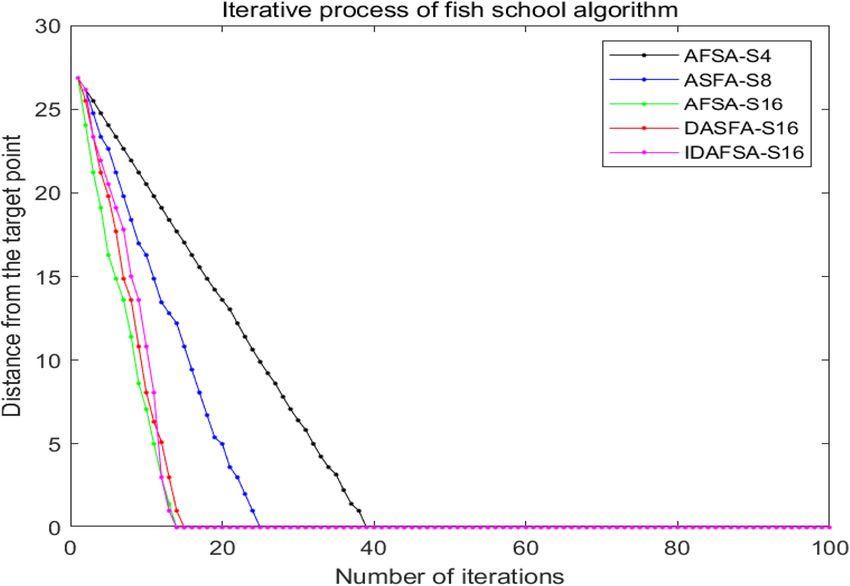
www.nature.com/scientificreports/

                                 Figure 2.  Grid environment matrix expression.

                                                                AXGEN

                                                               Xj

                                                                                     al
                                                                                     su
                                                                                  vi

                                                                       Xi
                                                                step

                                                                                            Xj

                                                   Xj

                                 Figure 3.  Artificial fish field of view model.


                                                                            f (x, y) =    (xi − xgoal )2 + (yi − ygoal )2                          (2)

                                 The artificial fish school algorithm and the Dijkstra algorithm.                     AFSA completes the process of
                                 finding the optimal solution by simulating the preying behavior, swarming behavior, following behavior, and
                                 random behavior of fish in nature. The artificial fish swarm mainly has the following parameters: the population
                                 size Nof the fish swarm, the position Xi (i = 1, 2, 3 . . . ., N) of the fish swarm, the food concentration Yc = f(xi)
                                 of the current position of the fish swarm, the crowding factor δ of the fish swarm, the number of attempts try-
                                 number of the fish swarm, the step size step of the fish swarm, the visual field range visual of the fish swarm,
                                 the distance between fish Xi and Xj is dij =� Xi − Xj �, and the maximum number of iterations MAXGEN. The
                                 model is shown in Fig. 3.

                                 Prey Behavior. Prey behavior is the most important behavior of the fish swarm algorithm. Artificial fish ran-
                                 domly select one location Xj in the field of vision, and compares the food concentration of current location Xi
                                 and location Xj. If the food concentration Yj of the random position is less than the food concentration Yi of
                                 the current position, position Xj will be reselected. Until the number of selections is greater than the number
                                 of attempts try-number of artificial fish, and no position with higher concentration than the current position is
                                 found, the random behavior is performed, and Eq. (3) is as follows:
                                                                                                      Xj (t) − Xi (t)
                                                                Xi (t + 1) = Xi (t) + step ∗                            ∗ rand()                   (3)
                                                                                                    � Xj (t) − Xi (t) �

Scientific Reports |   (2022) 12:659 |                  https://doi.org/10.1038/s41598-021-04506-y                                                   3

                                                                                                                                                Vol.:(0123456789)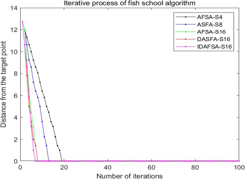
www.nature.com/scientificreports/

                                           Figure 4.  Dijkstra algorithm grid environment and its adjacency matrix.

                                           Swarm Behavior. Swarm behavior is a substantial way of survival for fish and can be used for collective forag-
                                           ing, as well as for the avoidance of natural enemies. There are two necessary conditions for aggregation behav-
                                           ior: one is close to the center of the fish group and the other is the low crowding degree of the fish group. By
                                                                                                                                               nf
                                           observing the number nf and position Xj of all fish in the field of vision, the center position Xc = j=1 Xj /nf is
                                           determined, and the concentration Yc is calculated. If the crowding degree nf /N ≤ δ of the current fish popula-
                                           tion and the concentration Yc of the center position is greater than Yi, indicating that the center position Xc is
                                           better and not crowded, clustering behavior can be performed; otherwise, foraging behavior can be performed.
                                           Equation (4) is as follows:
                                                                                                            Xc − Xi (t)
                                                                           Xi (t + 1) = Xi (t) + step ∗                   ∗ rand().                             (4)
                                                                                                          � Xc − Xi (t) �

                                           Follow Behavior. Artificial fish observe the fish within the field of vision, determine the optimal food concen-
                                           tration Yj and its position Xj, and are close to this position. If Yj is greater than the concentration Yi of the current
                                           position and the density nf /N ≤ δ of the current fish, this shows that the better position of Xj can perform the
                                           pursuit behavior; otherwise it can perform the foraging behavior. Equation (5) is as follows:
                                                                                                          Xj (t) − Xi (t)
                                                                         Xi (t + 1) = Xi (t) + step ∗                       ∗ rand().                           (5)
                                                                                                        � Xj (t) − Xi (t) �

                                           Random Behavior. Random behavior is a kind of default behavior for the fish swarm. In the visual field of artifi-
                                           cial fish, the random selection of a direction to move can prevent fish from lowing efficiency and local optimum,
                                           which is more conducive to the global optimum. The formula is expressed as follows:
                                                                                   Xi (t + 1) = Xi (t) + visual ∗ rand().                                       (6)

                                           Dijkstra algorithm. The core idea of the Dijkstra algorithm is to take the initial point as the center point,
                                           and continuously iteratively expand to the outer layer until the target point is found. Figure 4 shows the grid map
                                           of the Dijkstra algorithm and the expression form of its adjacency matrix, and INF represents the unreachable.

                                           Improved artificial fish swarm algorithm. In the traditional AFSA, there is a problem where the global
                                           optimal solutions and the local optimal solutions interfere with each other. To avoid the algorithm falling into
                                           a local optimum, and thus, unreasonable planning occurs, the feasible solution of the fish swarm is used to
                                           replace the optimal solution, meaning that the fish swarm path point of the target point is recorded. Among
                                           these feasible solutions, the shortest path is selected as the optimal solution, and it is used as the final route of
                                           path planning.                               √
                                               In the grid map, the step size range [1, 2] of the traditional artificial fish swarm algorithm is usually 4-Direc-
                                           tion 4-Neighborhood in Fig. 5a or 8-Direction 8-Neighborhood in Fig. 5b. However, to quickly reach the target
                                           position, it is necessary to increase the step size range.√   In the moving mode of 16-Direction 24-Neighborhood
                                           in this paper, the step size range of artificial fish is [1, 2 2], as shown in Fig. 6.
                                               Compared with the traditional step size range, the proposed step size range has more direction selection
                                           and a wider step size range, which is beneficial for artificial fish to quickly reach the target point. In the follow-
                                           ing, an example is used to illustrate the advantages of the proposed 16-Direction 24-Neighborhood contrast to
                                           the traditional step size range. As shown in Fig. 7, the existing fish swarm should reach Xj from Xi. Figure 7a, b
                                           are the paths planned by the traditional step size range. Figure 7c shows the planning path of the 16-Direction
                                           24-Neighborhood. If the length of a grid is expressed as 1, the iteration times and path lengths of different step
                                           sizes can be calculated, as shown in Table 1. Table 1 shows that the step size range of the 16-Direction 24-Neigh-
                                           borhood proposed in this paper can find shorter paths with fewer iterations.

          Scientific Reports |   (2022) 12:659 |                 https://doi.org/10.1038/s41598-021-04506-y                                                       4

Vol:.(1234567890)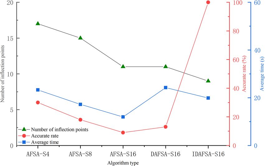
www.nature.com/scientificreports/

                                 Figure 5.  Step size range of the traditional fish school algorithm.

                                 Figure 6.  The step size range of the 16-Direction 24-Neighborhood.

                                                          Xj                                          Xj                       Xj

                                         Xi                                        Xi                           Xi
                                 (a) 4 directions of movement             (b) 8 directions of movement     (c) 16 directions of movement

                                 Figure 7.  The planned path of a non-synchronized long range.

                                  Step range                     Path length   Number of iterations
                                  4-Direction 4-Neighborhood     3.00          3
                                  8-Direction 8-Neighborhood     2.41          2
                                  16-Direction 24-Neighborhood   2.24          1

                                 Table 1.  Asynchronous long range result comparison.

Scientific Reports |   (2022) 12:659 |                  https://doi.org/10.1038/s41598-021-04506-y                                              5

                                                                                                                                           Vol.:(0123456789)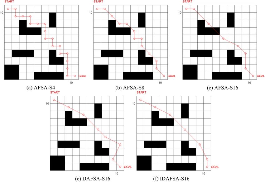
www.nature.com/scientificreports/
(a) (b) (c)
Figure 8. Irrational planning when the step range increases.
When the step range increases, obstacles may appear in the range, and fish can "surmount" the obstacles to
reach the target point. However, for 2-D planar mobile robots, obstacle crossing must not occur. For mobile
robots, the step size range proposed in this paper may lead to obstacle crossing, as shown in Fig. 8. The reason for
this situation is that the traditional fish swarm algorithm determines the step size range through the Euclidean
distance. However, with the increase in the step size range, the Euclidean distance cannot determine whether
there is an obstacle between the two positions, and thus, obstacle crossing behavior occurs. The Dijkstra algo-
rithm is introduced to confirm the step between two points as follows (7): If the equation is valid, there is no
obstacle between the two points. Otherwise, the point does not satisfy the step range condition and is deleted
from the neighborhood. However, when encountering the case in Fig. 8c, the Dijkstra algorithm is unable to
identify the obstacle. Thus, formula (8) is introduced to judge it
Xi − Xj = Dijkstra(Dmap, Xi , Xj ) (7)
Allow_area_i() ∩ Allow_area_j() = 2 (8)
√
Allow_area_i() represents the feasible region where the step size range of the current position Xi is 1, 2 ,
√
and Allow_area_j() is the feasible region where the random step size range of the neighborhood is 1, 2 . Dijk-
stra() is the Dijkstra algorithm and Dmap is the adjacency matrix of the grid map. In the traditional algorithm,
the probability of each attempt in each neighborhood is the same, thereby reducing the probability of a successful
attempt. Therefore, the culled factor is introduced, and the neighborhood that has been culled will no longer be
tried in the next attempt.
The artificial fish wants to reach Xj in the field of view, but due to the randomness of the artificial fish’s swim-
ming direction, it is necessary to determine whether the distance between the points in the neighborhood and Xj
is less than the distance between Xi and Xj, as shown in Fig. 9 below, and it is satisfied The neighborhoods of the
above conditions are all filled with colors, and the remaining neighborhoods are not satisfied. In the traditional
algorithm, the probability of each attempt in each neighborhood is the same, thereby reducing the probability
of successful attempts. Therefore, the elimination factor is introduced, and the unsatisfactory elimination bit
neighborhood will not be tried in the next attempt.
In the ASFA algorithm, the range of step size and field of vision are the main parameters affecting the con-
vergence speed of the algorithm. The range of fields of vision has a very important influence on other behaviors
of the fish swarm. The larger the range of the visual field, the more prominent the clustering behavior and fol-
lowing behavior of the fish swarm, which is beneficial for finding the global optimum. The small field of vision,
fish foraging behavior and random behavior are more prominent, and a small range search will be more careful,
but it will easily fall into a locally optimal solution. Therefore, the dynamic feedback field of vision is introduced
to adjust the field of vision by feedback of the distance from the current position to the target point. Therefore,
the fish can have a large field of vision in the early stage to quickly approach the target point. In the later stage,
the fish can search carefully with a small field of vision and quickly reach the target point. The specific formula
is as follows (9):
t
visual =
visual max ∗e
− ∗ T
dist (9)
= m ∗ 1 − DistMin
In the formula, visualmax is the maximum field of vision, m is the adjustable parameter, t is the current itera-
tion number, T is the maximum iteration number, dist is the Euclidean distance from the target point in the fish
swarm, DistMin is the Euclidean distance between the starting point and the endpoint, and λ is the feedback
factor, which can be more effective in adjusting the field of vision.
Scientific Reports | (2022) 12:659 | https://doi.org/10.1038/s41598-021-04506-y 6
Vol:.(1234567890)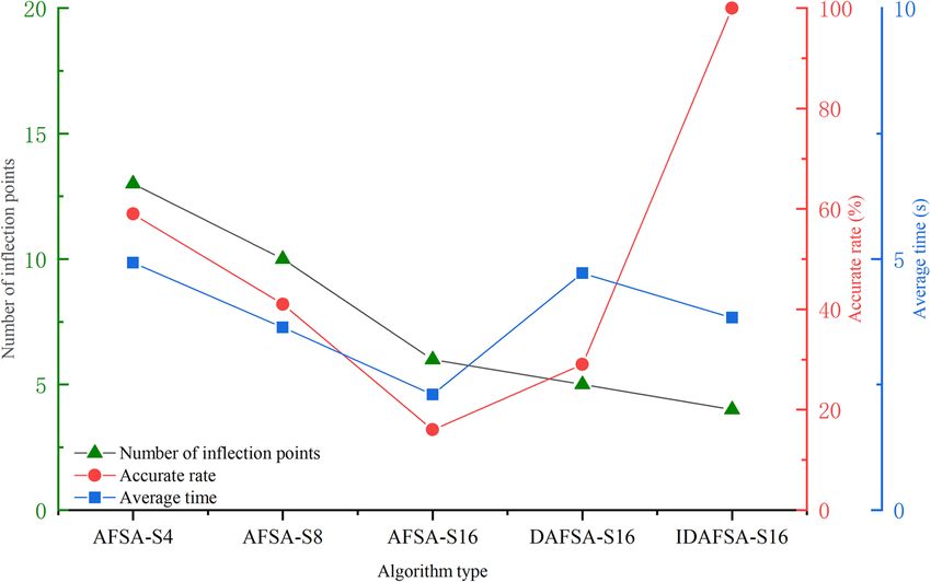
www.nature.com/scientificreports/
Xi
Xj
Figure 9. The range where artificial fish can try swim.
The larger the step range, the faster the algorithm will converge, but when it reaches a certain range, the larger
the step will oscillate, which will affect the convergence speed. Therefore, an adaptive step range is introduced.
When the field of vision is less than a certain value, the step range-specific formulas (10–11) are as follows:
step = α ∗ stepmin (10)
2 visual ≥ step max
α=
1 visual < step max (11)
In the formula, α is the adjustment factor, stepmin is the minimum step size range, and stepmax is the maximum
step size range.
The specific steps of the improved artificial fish swarm algorithm are shown in Fig. 10:
Step 1 We initialize the artificial fish parameters, such as the range of step length, range of vision, start point,
end point, number of attempts, number of populations, and the crowding factor.
Step 2 We initialize the location of the fish population.
Step 3 We share the barrier information if the sharing mechanism is satisfied; otherwise, we calculate the
barrier information.
Step 4 We perform preying behavior, swarming behavior, following behavior and random behavior and record
the location information of the fish simultaneously.
Step 5 If the target point is found, we find the optimal solution among feasible solutions and end the loop;
otherwise, we execute the next step.
Step 6 If the maximum number of cycles is reached, we end the cycle; otherwise, we return to step 3.
Path smoothing. Since the path planning in this paper was performed under the grid map, whose initial
path is composed of many folded line segments, there are places with sharp turns, where curvature and path
orientation discontinuity occurs. At these turning points, the continuity of curvature and path orientation must
be satisfied. The relationship between the radius of the rotation and curvature is as follows (12):
1 Ṗ(t) × P̈(t)
κ= = 3 (12)
R
Ṗ(t)
In this paper, the Bezier curve is used to smooth the path. In References19,20 , the n-order Bezier curve of n + 1
control points (P0, P1, . . . , Pn) is defined as follows:
n
n i
P(s) = PiBn, s(s), Bn, i(s) = s (1 − s)n−i (13)
i
i=0
In formula (17), s is 0 ≤ s ≤ 1, and Bn, i(s) are Bernstein polynomials.
Scientific Reports | (2022) 12:659 | https://doi.org/10.1038/s41598-021-04506-y 7
Vol.:(0123456789)www.nature.com/scientificreports/
Start
The state of artificial
fish
Initialization parameters, start and
end points
Improving
swarm behavior
Construct the artificial fish
population N
Improving prey
behavior
N
Is the sharing mechanism triggered? N
Y
Y Random
Calculate obstacle behavior
information Y
Sharing Barrier Information
Output
Improving Improving
Update visual and step
swarm behavior follow behavior
The state of artificial
fish
Select the higher concentration
point and update the information Improving
follow behavior
N
Y
Improving prey
Find the target?
behavior
N N
Computing the Y
Random
N shortest path
Reach the maximum number of iterations? behavior
Y
Y
Output
End
Figure 10. Flow chart of the improved artificial fish swarming algorithm.
In this paper, the third-order Bezier curve is used to smooth the path; each of the four control points controls
a curve. As shown in the above figure, E0, B0, B1, B2 and E2, A0, A1, A2 are the points passed by the planned paths
−−→ −−→ −−→
E0E1 and E1E2. E1 is the inflection point of the path, u1, u2 is the unit vector of E1 E0 and E1 E2 , C = (Cx , Cy ) = E0 E2
−−→ −−→ −−→ −−→
is the vector connecting E0 and E2, α and β are the angles of B2 A2 and B2 E1 , E0 E1 and E1 E2.
According to the smoothing theory of continuous third-order Bezier curves, the third-order Bezier curve
segments satisfy formula (14) as follows:
F(α) = cos2 (β − α) sin α[(c1 + 6 cos2 α)Dy
− 6Cx cos α sin α] + cos2 α sin(β − α)[c1 (Cy cos β (14)
− Cx sin β) + 6 cos (β − α)(Cy cos α − Cx sin α)] = 0
The above curve is composed of two Bezier curves and is determined by eight control points. The first curve
is controlled by four points as follows:
B = E1 + d1 u1
0
B1 = B0 − pb u1
(15)
B2 = B1 − qb u1
B3 = B2 − fb ud
The second curve is controlled by four points:
Scientific Reports | (2022) 12:659 | https://doi.org/10.1038/s41598-021-04506-y 8
Vol:.(1234567890)www.nature.com/scientificreports/
E2
A0
A1
C
A2
A3
B3 u2
α β
u1
E0 B0 B1 B2 E1
Figure 11. The Bezier curve model.
A = E1 + d2 u2
0
A1 = A0 − pa u2
(16)
A2
= A1 − qa u2
A3 = A2 − fa ud
−In
−→Eqs. (15) and (16) above, d1 and d2 are the lengths of E1B0 and E1A0 respectively, and ud is the unit vector
of B2 A2. Other parameters can be expressed by Eqs. (17.1–17.4) as follows:
pa = c2 qa
pb = c2 qb (17.1)
qa = qb cos2 α sin(β−α)
sin α cos2 (β−α)
(c2 +4)Cy cos2 (β−α)sinα (17.2)
q =
b [(c1 −6) cos α sin(β−α)+6 sin β] cos α sin β
6
fa = c2 +4 qa cos(β − α)
6 (17.3)
fb = c2 +4 qb cos α
c1 = 7.2364
√
c2 = 25 ( 6 − 1) (17.4)
To reduce the number of parameters, the mirror law is introduced so that d = d1 = d2, α = β/2; then from Fig. 11,
we obtain the Eq. (18) as follows:
Cx = l + l cos β
Cy = d sin β (18)
Substituting (18) into (14) to simplify gives Eq. (19) as follows:
F(α) = c1 d sin β[cos2 (β − α) sin α − cos2 α sin(β − α)]
β
+ 6d cos2 (β − α) sin α cos2 α sin β − cos2 sin 2α (19)
2
+ 6d cos2 α sin(β − α) cos(β − α)[sin(β − α) − sin α]
Substituting (18) into qa, qb, the Eqs. (20.1–20.3) obtained by simplifying as follows:
(c2 + 4))d sin 2α cos2 α sin α
qb = = c3 d (20.1)
[(c1 − 6) cos α sin α + 6 sin 2α] cos α sin 2α
qb cos2 α sin α
qa = = qb (20.2)
sin α cos2 α
Scientific Reports | (2022) 12:659 | https://doi.org/10.1038/s41598-021-04506-y 9
Vol.:(0123456789)www.nature.com/scientificreports/
Pi +1 Pi +2 Pi +3 goal
Pi
start
Figure 12. Collinear optimization of the path points.
c2 + 4
c3 = (20.3)
c1 + 6
Thus, simplifying Eqs. (17.1–17.4) yields the Eqs. (21.1–21.3) as follows:
qa = qb = c3 d (21.1)
pa = pb = c2 c3 d (21.2)
6c3 cos α
fa = fb = d (21.3)
c2 + 4
In Formula (21) above, as long as the size is determined, eight control points can be determined, and the
third-order Bezier curve can be constructed. In general, the first line of the two adjacent straight lines is used
to construct an arc satisfying the maximum rotation curvature. At the last point A of the first arc, the first and
second derivatives of the third-order Bezier curve are as follows (22):
−
→
Ṗ(1) = 3 fb
−
→ (22)
P̈(1) = 6 fb − 6−
→qb
By substituting formula (22) into (12), we can obtain the equation as follows:
−
→ −
→
3 fb × (6 fb − 6− →
qb )
2hb sin α
κmax = − =
→ 3 3fb2
3 fb (23)
(c2 + 4)3
sin α
=
54c3 d cos2 α
Therefore when d ≠ 0 or α ≠ 90°, the κmax of the third-order Bezier curve is continuous.
Because the planned path has multipoint collinearity, this situation does not meet the continuity condition
(α ≠ 90°) of the above three-order Bezier curve, so the intermediate redundant points are removed. In this paper,
the rank method of matrix is used to determine whether the three points (x1, y1), (x2, y2) and (x3, y3) are linearly
correlated as follows:
x1 y1 1
a = x2 y2 1 (24)
x3 y3 1
In Eq. (24), if a is a full rank matrix, then the three points are not collinear, then (x2, y2) is reserved, oth-
erwise (x2, y2) is discarded. In the algorithm, collinear optimization is carried out for the planned path. First,
the number of planned path points i is calculated, and the starting point is put into Final. Then, three points
P j−1 , Pj , Pj+1 (j = 2, 3 . . . , i − 1) are removed to judge whether they are collinear. If they are collinear, Pj
is put into Final, otherwise Pj is discarded until the end of the j + 1 > i cycle, and finally the target point is
put into Final. As shown in Fig. 12, the improved artificial fish swarm algorithm shows that the path points
are (start, Pi , Pi+1 , Pi+2 , Pi+3 , goal) and that the path points after the path passing collinear optimization are
(start, Pi+1 , goal), which satisfies the conditions of continuous third order Bezier curve.
Results
To verify the effectiveness and feasibility of the combination of the improved artificial fish swarm algorithm and
the continuous Bessel curve smoothing algorithm proposed in this paper, comparative simulation experiments
are carried out in grid environments with different complexities.
Comparison of artificial fish school algorithms. In a 10 × 10 grid map environment, several com-
parison experiments are carried out, and the basic parameters of the algorithm are the same, namely N = 50,
try-number = 8, MAXGEN = 100, visual = 5, and ∂ = 0.618. However, the swimming modes are 4-Direc-
Scientific Reports | (2022) 12:659 | https://doi.org/10.1038/s41598-021-04506-y 10
Vol:.(1234567890)www.nature.com/scientificreports/
Figure 13. Comparison of simulation plots of paths planned by different algorithms in a 10 × 10 grid
environment.
Algorithm Longest path Shortest path Average
AFSA-S4 18.0000 20.6051 18.6758
ASFA-S8 17.7568 14.8284 15.5852
ASFA-S16 16.4721 13.7726 14.2722
DASFA-S16 15.0711 13.7726 14.1289
IDAFSA-S16 14.1289 13.1869 13.5567
Table 2. Comparison of path lengths of different algorithms in a 10 × 10 grid environment.
tion 4-Neighborhood (AFSA-S4) and 8-Direction 8-Neighborhood (AFSA-S8), 16-Direction 24-Neighbor-
hood (AFSA-S16), Dijkstra-based 16-Direction 24-Neighborhood (DASFA-S16), and the improved DAFSA-
S16 algorithm√ (IDFSA-S16) √ is proposed in this paper. The basic parameters of IDAFSA-S16 are visualmax = 5,
stepmax = 2 2, stepmin = 2 , and m = 17. In a 10 × 10 grid environment, the paths planned by different algo-
rithms are shown in Fig. 13.
From the analysis of Table 2, Figs. 13, 14 and 15, the path planned by ASFA-S4 is too cumbersome, with too
many iterations and too much calculation. The average planning path length is relatively large and there are
many inflection points; the average planned path length of ASFA-S8 is reduced by 16.5% compared with that
of AFSA-S4, but the shortest and longest paths fluctuate greatly and unstable, with relatively many inflection
points. The average planning path length of AFSA-S16 is 23.6% and 8.4% less than that of AFSA-S4 and AFSA-
S8, respectively, with relatively fewer inflection points and the least number of operations, but it is not stable and
prone to unreasonable planning, and global solution oscillation occurs due to the large range of the later field of
view, which affects the algorithm’s later optimization search.DAFSA-S16 introduces Dijkstra algorithm on the
basis of AFSA-S16. DAFSA-S16 introduces the Dijkstra algorithm on the basis of AFSA-S16 to further confirm
the obstacle information within the step length, and the simulation results show that the accuracy of the algo-
rithm is improved. At the same time, the average path length of DAFSA-S16 is reduced by 24.3%, 9.3%, and 1.0%
compared with AFSA-S4, AFSA-S8, and AFSA-S16, respectively, and the inflection point is also relatively small.
Scientific Reports | (2022) 12:659 | https://doi.org/10.1038/s41598-021-04506-y 11
Vol.:(0123456789)www.nature.com/scientificreports/
Figure 14. Comparison of the number of inflection points, average time and planning accuracy of different
algorithms in a 10 × 10 grid environment.
Figure 15. Comparison of the number of iterations of different algorithms in a 10 × 10 grid environment.
Since the large field of vision in the late stage will affect the optimization of the algorithm, the late oscillation of
the algorithm shown in Fig. 13d above appears. IDSFA-S16 can effectively solve the behavior of unreasonable
crossing of the planning path, while the feedback field of view range can effectively solve the problem of global
solution oscillation at the later stage of the algorithm. The average path length is 27.4%, 13%, 5.0%, 4.0% less
than the above algorithm, and the accuracy of the algorithm planning can also reach 100%, while the inflection
point is relatively less, and the path is smoother, but the amount of operations is relatively increased.
In a 20 × 20 grid map environment, several comparison experiments are carried out, and the basic parameters
of the algorithm are the same, namely, N = 50, try-number = 8, MAXGEN = 100, visual = 5, and ∂ = 0.618. However,
the swimming modes are 4-Direction 4-Neighborhood (AFSA-S4) and 8-Direction 8-Neighborhood (AFSA-S8),
16-Direction 24-Neighborhood (AFSA-S16), Dijkstra-based 16-Direction 24-Neighborhood (DASFA-S16), and
Scientific Reports | (2022) 12:659 | https://doi.org/10.1038/s41598-021-04506-y 12
Vol:.(1234567890)www.nature.com/scientificreports/
Algorithm Longest path Shortest path Average
AFSA-S4 43.2366 39.2361 39.5647
ASFA-S8 31.2132 29.2132 30.6538
ASFA-S16 34.9494 27.9367 29.6522
DASFA-S16 30.9596 28.7814 29.5581
IDAFSA-S16 30.4361 29.2648 29.4916
Table 3. Comparison of planned path lengths in a 20 × 20 grid environment.
Figure 16. Comparison of simulation plots of paths planned by different algorithms in a 20 × 20 grid
environment.
the improved DAFSA-S16 algorithm √ (IDFSA-S16) √ proposed in this paper. The basic parameters of IDAFSA-
S16 are visualmax = 5, stepmax = 2 2, stepmin = 2 , and m = 10. Table 3 shows the comparison of planned path
lengths in a 20 × 20 grid environment, Fig. 16 shows the planning path under the grid environment of 20 × 20,
and Fig. 17 shows the comparison iteration diagram.
The analysis of Table 3, Figs. 16, 17 and 18 shows that in the relatively complex environment, the path planned
by AFSA-S4 is very complex, with the largest number of inflection points and iterations, as well as the larg-
est number of algorithm operations. There is also an unreasonable cross-barrier phenomenon. The difference
between the longest path and the shortest path planned by ASFA-S8 is large, and the global optimal solution and
the local optimal solution interfere with each other, leading to unreasonable planning paths. AFSA-S16 is dif-
ficult to plan the route correctly. DAFSA-S16 planning accuracy is improved, and the inflection point is relatively
small, but it is also difficult to control the local optimum and the global optimum interfering with each other. By
replacing the optimal solution with a feasible solution, IDAFSA-S16 can ensure rationality and stability under
the planned path, while also reducing the number of inflection points and the number of iterations. Then, the
algorithm operations are relatively reduced, and the average path lengths are 25.4%, 3.9%, 0.5% and 0.2% less
than those of the above algorithms.
Path Smoothing. To verify the effectiveness of the path smoothing of the third-order Bessel curve and the
continuity after collinear optimization, simulations are carried out in grid environments with different com-
Scientific Reports | (2022) 12:659 | https://doi.org/10.1038/s41598-021-04506-y 13
Vol.:(0123456789)www.nature.com/scientificreports/
Figure 17. Comparison of the number of iterations of different algorithms in a 20 × 20 grid environment.
Figure 18. Comparison of the number of inflection points, average time and accuracy of different algorithms in
a 20 × 20 grid environment.
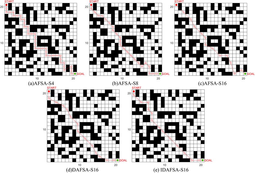
plexities, as shown in Fig. 19. From the simulation results, it can be seen that in different environments, by intro-
ducing the third-order Bessel curve, the path is smoothed so that the original sharp inflection point becomes
smooth, and the actual control meets the kinematic and dynamic characteristics of the mobile robot. By effec-
tively avoiding obstacles and satisfying feasibility, the continuity of the rotation angle and path curvature of the
mobile robot is realized.
Discussion and conclusion
Aiming at robot path planning, this paper proposed a method combining third-order Bessel curves with an
improved artificial fish swarm algorithm. First, morphological processing, such as the expansion of obstacles,
was carried out, and during the path planning process, an artificial fish swimming range of 16 directions and 24
fields based on Dijkstra’s algorithm was introduced to provide the movement rules of the artificial fish, which
Scientific Reports | (2022) 12:659 | https://doi.org/10.1038/s41598-021-04506-y 14
Vol:.(1234567890)www.nature.com/scientificreports/
Figure 19. Simulation of path smoothing in different raster environments.
improves the accuracy of planning while reducing the inflection points. At the same time, by adding the sharing
mechanism, the number of operations of the fusion algorithm was reduced. By introducing the feasible solu-
tion, the problem of mutual interference between the local optimal solution and the global optimal solution was
solved. By introducing the feedback field of view range, the oscillation phenomenon caused by an excessively
large field of view in the later stage of the algorithm was avoided. The improved artificial fish swarm algorithm
proposed in this paper generates a collision-free, inflection-point less and shorter path connected by a sequential
sequence of path points. Finally, smoothing by using the theory of cubic Bessel curves ensures the continuity of
direction and curvature of any point on its path, while made it satisfy the minimum rotation radius to reduce
the mechanical structure damage of the robot. By comparing the simulation results of the proposed algorithm
with the traditional fish swarm algorithm, it can be seen that the proposed fusion algorithm had the shortest
average path, the least number of inflection points, and was more consistent with the kinematic characteristics
of the robot, while also ensured a 100% correct planning rate. At the same time, the proposed fusion algorithm
introduces Dijkstra’s algorithm, which causes an increase in computation, but then the fish sharing mechanism
was introduced to offset part of the computation.
In summary, it is sufficient to prove the effectiveness and superiority of the proposed algorithm in this paper.
However, the proposed algorithm was only tested in a raster environment and not in a real environment. In
future work, we will conduct experiments and debugging in a real environment. We are also interested in using
IDAFSA in multirobot collaborative path planning.
Received: 5 October 2021; Accepted: 23 December 2021
References
1. Atyabi, A. & Powers, D. Review of classical and heuristic-based navigation and path planning approaches. Int. J. Adv. Comput.
Technol. 5, 66 (2013).
2. Wang, Q. & Wang, Y. Route planning based on combination of artificial immune algorithm and ant colony algorithm. Found. Intell.
Syst. 66, 121–130 (2011).
3. Neshat, M., Pourahmad, A. A. & Rohani, Z. Improving the cooperation of fuzzy simplified memory A* search and particle swarm
optimisation for path planning. Int. J. Swarm Intell. 5, 1–21 (2020).
4. Duchoň, F. et al. Path planning with modified a star algorithm for a mobile robot. Procedia Eng. 96, 59–69 (2014).
5. Sheng, J. et al. An improved artificial potential field algorithm for virtual human path planning. In International Conference on
Technologies for E-Learning and Digital Entertainment 592–601 (Springer, 2010).
6. Jianguo, W. et al. Path planning of mobile robot based on improving genetic algorithm. In Proceedings of the 2011 International
Conference on Informatics, Cybernetics, and Computer Engineering (ICCE2011) November 19–20, Melbourne, Australia 535–542
(Springer, 2011).
7. Guo, N. et al. Local path planning of mobile robot based on long short-term memory neural network. Autom. Control. Comput.
Sci. 55, 53–65 (2021).
8. Chen, X. et al. Unmanned ship path planning based on RRT. In International Conference on Intelligent Computing 102–110
(Springer, 2018).
9. Neshat, M. et al. Artificial fish swarm algorithm: A survey of the state-of-the-art, hybridization, combinatorial and indicative
applications. Artif. Intell. Rev. 42, 965–997 (2014).
10. Xiao, J. et al. A modified artificial fish-swarm algorithm. In 2006 6th World Congress on Intelligent Control and Automation, 1,
3456–3460 (IEEE, 2006).
11. Wang, J. & Wu, L. J. Robot path planning based on artificial fish swarm algorithm under a known environment. Adv. Mater. Res.
989, 2467–2469 (2014).
12. Zhang, C. et al. Improved artificial fish swarm algorithm. In 2014 9th IEEE Conference on Industrial Electronics and Applications
748–753 (IEEE, 2014).
13. Huang, Y. et al. Path planning of mobile robots based on logarithmic function adaptive artificial fish swarm algorithm. In 2017
36th Chinese Control Conference (CCC) 4819–4823 (IEEE, 2017).
14. Qi, B. et al. A weights and improved adaptive artificial fish swarm algorithm for path planning. In 2019 IEEE 8th Joint International
Information Technology and Artificial Intelligence Conference (ITAIC) 1698–1702 (IEEE, 2019).
15. Hu, X. T., Zhang, H. Q., Li, Z. C., Huang, Y. A. & Yin, Z. P. A novel self-adaptation hybrid artificial fish-swarm algorithm. IFAC
Proc. Vol. 46, 583–588 (2013).
Scientific Reports | (2022) 12:659 | https://doi.org/10.1038/s41598-021-04506-y 15
Vol.:(0123456789)www.nature.com/scientificreports/
16. Tirkolaee, E. B., Goli, A. & Weber, G.-W. Fuzzy mathematical programming and self-adaptive artificial fish swarm algorithm for
just-in-time energy-aware flow shop scheduling problem with outsourcing option. IEEE Trans. Fuzzy Syst. 28, 2772–2783 (2020).
17. Gilimyanov, R. F. Recursive method of smoothing curvature of path in path planning problems for wheeled robots. Autom. Remote.
Control. 72, 1548–1556 (2011).
18. Lekkas, A. M. & Fossen, T. I. Integral LOS path following for curved paths based on a monotone cubic Hermite spline parametriza-
tion. IEEE Trans. Control Syst. Technol. 22, 2287–2301 (2014).
19. Aldair, A. A., Rashid, M. T. & Rashid, A. T. Navigation of mobile robot with polygon obstacles avoidance based on quadratic bezier
curves. Iran. J. Sci. Technol. Trans. Electric. Eng. 43, 757–771 (2019).
20. Tharwat, A. et al. Intelligent Bézier curve-based path planning model using chaotic particle swarm optimization algorithm. Clust.
Comput. 22, 4745–4766 (2019).
Author contributions
F.-F.L. designed and conducted the experiment and wrote the manuscript. Dr. Y.D. supervised whole project.
Dr. K.-J.J. supervised whole project.
Funding
This work was financially supported by the Key Research and Development Program Projects in Hebei Province
(19221814D); Shijiazhuang Science and Technology Research and Development Plan (211130143A).
Competing interests
The authors declare no competing interests.
Additional information
Correspondence and requests for materials should be addressed to K.-J.J.
Reprints and permissions information is available at www.nature.com/reprints.
Publisher’s note Springer Nature remains neutral with regard to jurisdictional claims in published maps and
institutional affiliations.
Open Access This article is licensed under a Creative Commons Attribution 4.0 International
License, which permits use, sharing, adaptation, distribution and reproduction in any medium or
format, as long as you give appropriate credit to the original author(s) and the source, provide a link to the
Creative Commons licence, and indicate if changes were made. The images or other third party material in this
article are included in the article’s Creative Commons licence, unless indicated otherwise in a credit line to the
material. If material is not included in the article’s Creative Commons licence and your intended use is not
permitted by statutory regulation or exceeds the permitted use, you will need to obtain permission directly from
the copyright holder. To view a copy of this licence, visit http://creativecommons.org/licenses/by/4.0/.
© The Author(s) 2022
Scientific Reports | (2022) 12:659 | https://doi.org/10.1038/s41598-021-04506-y 16
Vol:.(1234567890)You can also read