Performance Engineering for the SKA telescope - PeterJBraam Mar2018 SKA Science Data Processor Cavendish Laboratory, Cambridge University - ICPE 2018
←
→
Page content transcription
If your browser does not render page correctly, please read the page content below
Performance Engineering
 for the SKA telescope
Peter J Braam                                Mar 2018
SKA Science Data Processor
Cavendish Laboratory, Cambridge University
peter.braam@peterbraam.com

Acknowledgement

A large group of people (~500) are working on this project
Most information is publicly available, but very technical
This presentation re-uses much from other SKA efforts

Particularly I’m using a few slides from Peter Wortmann
Background: skatelescope.org

My role: consultant & visiting acaemic for Cambridge group since 2013

                                                                        2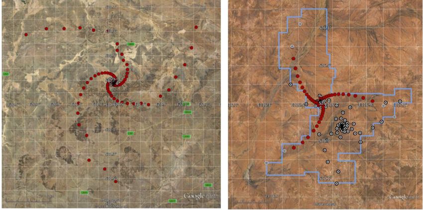
Message from this talk
1. SKA telescope is a grand challenge scale project

2. Synergy between scientific computing and industry for performance

    Hardware – particularly memory, energy

    Software – agility, parallelism, energy

3. General purpose tools appear insufficient, there may be fairly deep open issues

                                                                                     3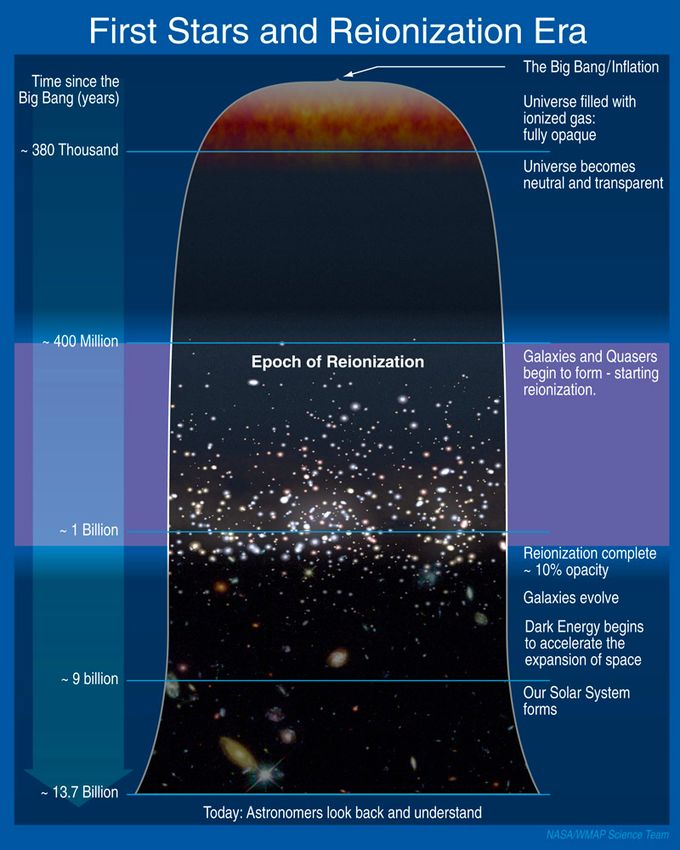
What is the SKA?

                   4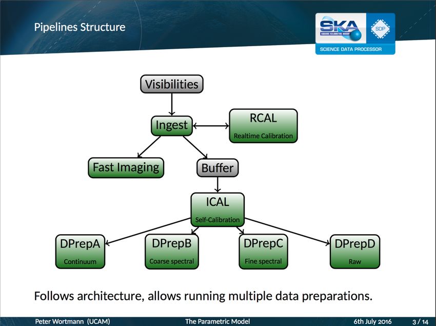
The Square Kilometre Array (SKA)
Next Generation radio telescope – compared to best current instruments it will offer
…
▪ ~ 100 times more sensitivity
▪ ~ 106 times faster imaging the sky
▪ More than 5 square km of collecting area over distances of >100km

Will address some of the key problems of astrophysics and cosmology (and physics)

▪ Builds on techniques developed originally in Cambridge
▪ It is an Aperture Synthesis radio telescope (“interferometer”)

Uses innovative technologies...

▪ Major ICT project
▪ Need performance at low unit cost
                                                                                       5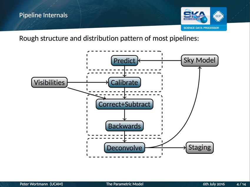
6
SKA – a partner to ALMA, EELT, JWST
  ALMA:                                            European ELT
  • 66 high precision sub-mm                       • ~40m optical telescope
  antennas                                         • Completion ~2025
  • Completed in 2013                              • ~$1.3 bn
  • ~$1.5 bn

 Credit:A.                                       Credit:ESO/L. Calçada (artists impression)
 Marinkovic/XCam/ALMA(ESO/NAOJ/NRAO)

  JWST:                                            Square Kilometre Array
  • 6.5m space near-infrared                       – phase 1
  telescope                                        • Two next generation
  • Launch 2018                                    antenna arrays
  • ~$8 bn                                         • Completion ~2025
                                                   • $0.80 bn

 Credit: Northrop Grumman (artists impression)   Credit: SKA Organisation (artists impression)   7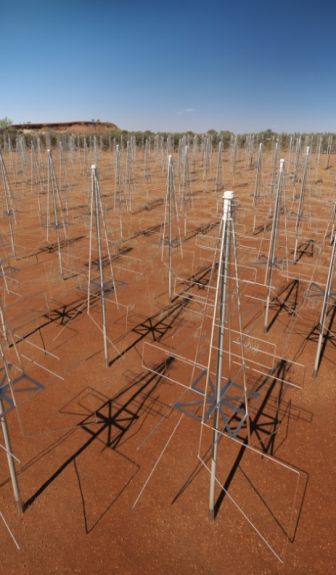
In summary …
▪ SKA aims to be a world class “instrument” like CERN

▪ SKA Phase 1 – in production 2025
▪ SKA Phase 2 – likely 10x more antennas – 2030’s?

▪ This presentation focuses on SKA1

▪ Caveat
  ▪ Ongoing changes
  ▪ Some inconsistencies in the numbers

                                                        8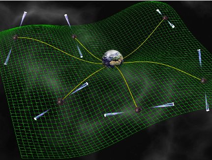
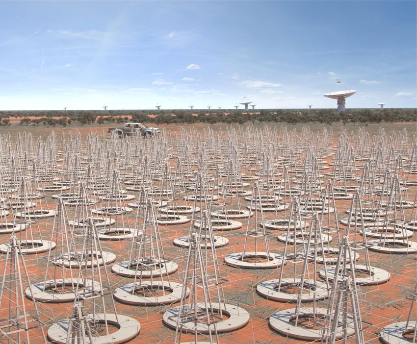
Low Frequency
Aperture Array
0.05 – 0.5 GHz

Australia

~1000 stations
256 antennas each
phased array with
Beamformers

Murchison Desert
0.05 humans/km2
Compute in Perth

                    9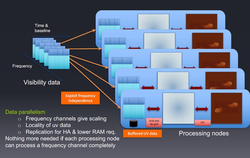
Mid Frequency Telescope

South Africa

250 dishes with single receiver
Karoo Desert, SA - 3 humans / km2
Compute in Cape Town (400 km)       10
Antenna array layout

SKA1–MID, –LOW: Max Baseline = 156km, 65 km

                                              11
Science
12Science Headlines
Fundamental Forces & Origins
Particles
Gravity Galaxy & Universe
▪ Radio Pulsar Tests of General ▪ Cosmic dawn
Relativity ▪ First Galaxies
▪ Gravitational Waves ▪ Galaxy Assembly & Evolution
▪ Dark Energy / Dark Matter
Stars Planets & Life
Magnetism
▪ Protoplanetary disks
▪ Cosmic Magnetism ▪ Biomolecules
▪ SETI
13
skatelescope.org – two very large books (free!) with science research articles surrounding SKAEpoch of
Re-Ionisation
21 cm Hydrogen
spectral line (Hl)
Difficult to detect
Tells us about the dark
age:
400K – 400M years
(current age 13.5G
year)
14Pulsar Timing Array
What can be found:
• gravitational waves
• Validate cosmic censorship
• Validate “no-hair” hypothesis
• Nano-hertz frequency range
• ms pulsars, fluctuations of 1 in 10^20
• SKA1 should see all pulsars (estimated ~30K) in our galaxy
15Physics & Astrophysics
Many key questions in theoretical physics relate to astrophysics
Rate of discoveries in the last 30 years is staggering
16Imaging Problem
17Standard interferometer
s
Astronomical signal
(EM wave)
B.s
Visibility V(B): what is measured on baselines
Detect &
amplify Image I(s): image
Solve for I(s)
1 B 2
Digitise & V(B) = E1 E2* = I(s) exp(i ω B.s/c) – image equation
delay
Correlate Maximum baseline gives resolution: θmax ~ λ / Bmax
X X X X X X Dish size determines Field of View (FoV): θdish ~ λ / D
Integrate
Process Calibrate, grid, FFT
SKY Image 18Interferometry radio telescope
Simplified
Sky is flat
Earth is flat
Telescope to image is Fourier transform
Actually
Sky is sphere, earth rotates, atmosphere
distorts
Now it is a fairly difficult problem:
1. Non-linear phase
2. Direction, frequency, baseline dependent
gain factor
19Data in the computation
Two principal data types
input is visibility – irregular, sparse uvw - grid of baselines
Image grid - regular grid in sky image
Different kinds of locality
Splitting the stream by frequency
Tiling visibilities by region – but visibility “tile” data is highly irregular
Analyze visibility structure – 0, sparse, dense: separate strategies
Remove 3rd dimension by understanding earth rotation
Data flow model with overlapping movement and computation
20Reducing to 2D Try to go back from 2D to 3D problem by relating (~100) different w values. Domain specific optimization. Grid size is 64K x 64K for 64K frequencies – problem is large Full FFT is O(k log k), sparse FFT: O(#nonzero log #nonzero). This approach is close to this. 21
Computing in radio astronomy - 101
@Antennas: wave guides, clocks, beam-forming, digitizers

@Correlator (CSP central signal processing): == DSP for antenna data
       Delivers data for every pair of antenna’s (a “baseline”)
       Dramatically new scale for radio astronomy ~100K baselines
       Correlator averages and reduces data, delivers sample every 0.3 sec
       Data is delivered in frequency bands: ~64K bands
       3 complex numbers delivered / band / 0.3 sec / baseline
       Do math: ~ 1 TB/sec input of so called visibility data

@Science Data Processor (SDP) – process correlator data
       Create images (6 hrs) & find transients (5 secs) – “science products”
       Adjust for atmospheric and instrument effects calibration               22
Outline of algorithm
About 5 different analysis on the data are envisaged:
e.g. spectral vs continuum imaging etc.
Imaging pipelines:
§ Iterate until convergence – approximately 10 times
§ Compares with an already known model of the sky
§ Incorporates and recalculates calibration data
2324
25
SDP specific Pipelines
Algorithmic similarities with other image processing
Each step is
         ▪ Convolution with some kind of a “filter” – e.g. “gridding”
         ▪ Fourier transform
         ▪ All-to-all for calibration

Why new & different software?
▪ Data is very distinct from other image processing
▪ Problem is very large – much bigger than RAM
▪ Reconstruction dependencies: sky model & calibration

                                                                        26
Engineering Problem
27Requirements & Tradeoffs
Turn telescope data into science products soft real time
1. Transient phenomena: time scale of ~10 seconds
2. Images: 1 image ~6 hours
Agility for software development
Telescope lifetime ~50 years
SDP computing hardware refresh ~5 years
Use of large clusters is new in radio astronomy
New telescopes always need new algorithms
Initial 2025 computing system goal: make SKA #1
So – how difficult is this?
28Flops vs. #channels & baseline
29SDP “performance engineering” approach
Conservative - this is not computing research
Known-good algorithms, hardware
Perhaps deep math question remains: is problem really O(#antennas^2)?
Parametric model of the computation
Detailed FLOPs, memory use, data movement, energy
Key outcome: 100 PF/sec & move 200 PB/sec from HBM to CPU
@50 PJ / byte this is ~10MW power
Software
Reference Libraries with Algorithms
Address scalability issues
30Relative kernel cost
31Software Framework for SKA SDP
Creating software is a very high risk part of the project
Ideal perspective:
Execution framework from 3rd party
Domain specific application language for pipelines
Automatic optimization – performance & energy
…. this is proving less easy than we had hoped
Many approaches – excellent compilers and ….
Adapting existing packages – MPI C++ applications
Use a big-data framework like Spark, TensorFlow
Use HPC frameworks like Swift/T, Legion
32Co-design
Foundations Hardware
Algorithms Systems
Lesson:
Interactions between these domains
Software is a very big challenge
33Work Breakdown
Foundations: be conservative – no totally new approaches
Algorithms: innovation - adapt to scale
Software: prototyping, seeking mainstream solution
Hardware: much has been learned from working with the chip vendors
Systems: analysis by HPC experts, costing, vendor ideas etc.
34Samples of Data Processing Considerations
35SKA – data schematic
Antennas Central Signal Imaging (SDP) – HPC problem
Processing (CSP) 2024: 100 PBytes/day
2030: 10,000 PBytes/day
Over 100’s kms
Transfer antennas to CSP
2024: 20,000 PBytes/day
2030: 200,000 PBytes/day
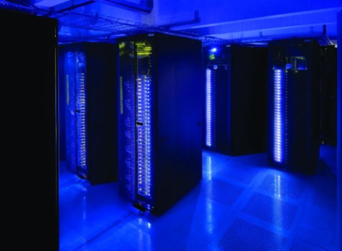
Over 10’s to 1000’s kms High Performance
Computing Facility (HPC)
HPC Processing
2024: 300 PFlop
In: 20 EB in -> out: 100 TB 2030: 30 EFlop 36SDP top-level compute challenge
Telescope Manager
Science Data Processor
SDP Local Monitor & Control
Long Term Delivery System
Data Processor
Archive
C Distribution
S High Performance
EB volume ~100PB/y
P ~100 PF/sec
~200 PB/sec
100PB annually From Cape Town &
Data Intensive
Perth to rest of
~100 PB/job
Infrequent World
Partially real-time
~10s access
Visualization of
Read-intensive
100k x 100k x 100k
Constrained 37
voxel cubesData Movement
Primarily compute
pipeline steps
10-30% efficiency Processing Elements: 100 PF/sec
200 PB/sec memory bandwidth
Primarily contains grid
data (64Kx64K) at 64K
frequencies Memory: ~1TB/node
10 TB/sec read bandwidth
Buffer: 25 PB/obs > ~50PB capacity
1 TB/sec ingest I/O
38Supercomputer parameters
2025 LFAA (AU) Mid (SA)
FLOPS 100 PF 360 PF
Memory Bandwidth
Memory bandwidth 200 Pb/sec 200 Pb/sec - Cost
- Energy
Buffer Ingest 7.3 TB/s 3.3 TB/s - 10x 1st EF BW
Budget 45 M€ 3.3 TB/s
Power 3.5 MW 2 MW
Buffer storage 240 PB 30 PB
Storage / node 85 TB 5 TB
Archive storage 0.5 EB 1.1 EB
39Memory … SKA’s biggest challenge
High Bandwidth Memory (HBM) is becoming dominant for HPC
In 2013 the problem looked perhaps out of reach
HBM is 3D, on package, memory
10x bandwidth of RAM, perhaps similar cost
Delay in SKA the deliverables has been very helpful
40Data Flow on System Architecture
41Visibilities & Baselines distribution
Each pair of telescopes has a
baseline
Baselines rotate as time
progresses
Each baseline has associated
visibility data (“sample”)
Baselines are sparse & not
regular, but totally predictable
The physical data structure
strongly enables and
constrains concurrency &
parallelism Simulated data from 250 SKA1-MID dishes
42Visibility gridding & cache re-use
Time rotation of
UV grid.
Only fetch edges
Re-use core
43Long vs short buffer question
Processing requires up to 6 hours of ingest – buffer that.
21,600 TB – “unit of data ingest” to compute on Buffer
memory
Overlapping ingest and compute: double buffer ?
Ingesting buffer Processing buffer
Double Buffer: ~50PB, write 1TB/sec, read 10TB/sec
But processing time is uneven –
double buffer: minimizes storage cost,
at expense of equally quick execution of worst compute costStream fusion
Some kernels exchange too much data
Solution: deviate from pipeline actors
do more operations and less data movement.
Few compilers / frameworks automatically
Doing it manually is awkward for portabilityConclusions
46Conclusions
Computing is extremely central, well beyond the instrument
e.g. applying AI / ML to analyzing the science data
Astrophysics has everyone’s attention – this project must succeed
SKA will succeed based on astrophysics
but its computing lies on the frontier of big data handling
Software may is the highest risk and hardest problem of all
47Thank you.
questions?
skatelescope.org
peter.braam@peterbraam.com
48You can also read