Numerical and Scientific Computing in Python - v0.1 Spring 2019 Research Computing Services

Numerical and Scientific Computing in Python

 v0.1
 Spring 2019

 Research Computing Services
 IS & T

Running Python for the Tutorial

 If you have an SCC account, log on and use Python
 there.
  Run:

module load python/3.6.2
spyder &
unzip /projectnb/scv/python/NumSciPythonCode_v0.1.zip

  Note that the spyder program takes a while to load!

Links on the Rm 107 Terminals

 On the Desktop open the folder:
 Tutorial Files  RCS_Tutorials  Tutorial Files

 Copy the whole Numerical and Scientific Computing in Python folder to
 the desktop or to a flash drive.
  When you log out the desktop copy will be deleted!

Run Spyder

 Click on the Start Menu in
 the bottom left corner and
 type: spyder

 After a second or two it will
 be found. Click to run it.

 Be patient…it takes a while
 to start.

Outline
 Python lists

 The numpy library

 Speeding up numpy: numba and numexpr

 Libraries: scipy and opencv

 Alternatives to Python

Python’s strengths

 Python is a general purpose language.
  Unlike R or Matlab which started out as specialized languages

 Python lends itself to implementing complex or specialized algorithms for
 solving computational problems.

 It is a highly productive language to work with that’s been applied to
 hundreds of subject areas.

Extending its Capabilities
 However…for number crunching some aspects of the language are not
 optimal:
  Runtime type checks
  No compiler to analyze a whole program for optimizations
  General purpose built-in data structures are not optimal for numeric calculations

 “regular” Python code is not competitive with compiled languages (C, C++,
 Fortran) for numeric computing.

 The solution: specialized libraries that extend Python with data structures
 and algorithms for numeric computing.
  Keep the good stuff, speed up the parts that are slow!

Outline
 The numpy library

 Libraries: scipy and opencv

 When numpy / scipy isn’t fast enough

NumPy

 NumPy provides optimized data structures and basic routines for
 manipulating multidimensional numerical data.

 Mostly implemented in compiled C code.

 Can be used with high-speed numeric libraries like Intel’s MKL

 NumPy underlies many other numeric and algorithm libraries available for
 Python, such as:
  SciPy, matplotlib, pandas, OpenCV’s Python API, and more

Ndarray – the basic NumPy data type

 NumPy ndarray’s are:
  Typed
  Fixed size (usually)
  Fixed dimensionality
 An ndarray can be constructed from:
  Conversion from a Python list, set, tuple, or similar data structure
  NumPy initialization routines
  Copies or computations with other ndarray’s
  NumPy-based functions as a return value

ndarray vs list

 List:  Ndarray:
  General purpose  Intended to store and process
  Untyped (mostly) numeric data
  1 dimension  Typed
  Resizable  N-dimensions
  Add/remove elements anywhere  Chosen at creation time
  Accessed with [ ] notation and  Fixed size
 integer indices  Chosen at creation time
  Accessed with [ ] notation and
 integer indices

List Review
 # Make a list
 x = []
 The list is the most common data structure in Python.
 # Add something to it
 Lists can: x.append(1)
  Have elements added or removed x.append([2,3,4])
  Hold any type of thing in Python – variables, functions, objects, etc. print(x)
  Be sorted or reversed
  Hold duplicate members --> [1, [2, 3, 4]]
  Be accessed by an index number, starting from 0.

 Lists are easy to create and manipulate in Python.

List Review x = ['a','b',3.14]

Operation Syntax Notes

Indexing – starting from 0 x[0]  ‘a’

 x[1]  ‘b’
Indexing backwards from -1 x[-1]  3.14

 x[-3]  ‘a’
Slicing x[start:end:incr] Slicing produces a COPY of
 the original list!
 x[0:2]  [‘a’,’b’]

 x[-1:-3:-1]  [3.14,’b’]

 x[:]  [‘a’,’b’,3.14]
Sorting x.sort()  in-place sort Depending on list contents a
 sorted(x)  returns a new sorted list sorting function might be req’d

Size of a list len(x)

List Implementation x = ['a','b',3.14]

 A Python list mimics a linked list data structure
  It’s implemented as a resizable array of pointers to Python objects for performance reasons.

 Pointer to a
 Python object
 'a'
 Allocated
 Pointer to a
 x Python object
 'b' anywhere in
 memory

 Pointer to a
 Python object
 3.14

 x[1]  get the pointer at index 1  resolve pointer to the Python object
 in memory  get the value from the object


import numpy as np
 # Initialize a NumPy array
NumPy ndarray # from a Python list
 y = np.array([1,2,3])

 The basic data type is a class called ndarray.
 The object has:
  a data that describes the array (data type, number of dimensions, number of elements, memory
 format, etc.)
  contiguous array in memory containing the data.
 Values are
 Data description physically
 (integer, 3 elements, 1-D) adjacent in
 y memory

 1 2 3
 y[1]  check the ndarray data type  retrieve the value at offset 1 in the
 data array
 https://docs.scipy.org/doc/numpy/reference/arrays.html

dtype
 Every ndarray has a dtype, the type a = np.array([1,2,3])
 of data that it holds. a.dtype  dtype('int64')
 This is used to interpret the block of
 data stored in the ndarray.
 c = np.array([-1,4,124],
 Can be assigned at creation time: dtype='int8')
 c.dtype --> dtype('int8')

 Conversion from one type to
 another is done with the astype()
 method: b = a.astype('float')
 b.dtype  dtype('float64')

Ndarray memory notes
 The memory allocated by an ndarray:

  Storage for the data: N elements * bytes-per-element
  4 bytes for 32-bit integers, 8 bytes for 64-bit floats (doubles), 1 byte for 8-bit characters etc.

  A small amount of memory is used to store info about the ndarray (~few dozen bytes)

 Data storage is compatible with external libraries
  C, C++, Fortran, or other external libraries can use the data allocated in an ndarray directly without
 any conversion or copying.

ndarray from numpy initialization

 There are a number of initialization routines. They are mostly copies of
 similar routines in Matlab.
 These share a similar syntax:
 function([size of dimensions list], opt. dtype…)

  zeros – everything initialized to zero.
  ones – initialize elements to one.
  empty – do not initialize elements
  identity – create a 2D array with ones on the diagonal and zeros elsewhere
  full – create an array and initialize all elements to a specified value
 Read the docs for a complete list and descriptions.

x = [1,2,3]
ndarray from a list y = np.array(x)

 The numpy function array creates a new array from any data structure
 with array like behavior (other ndarrays, lists, sets, etc.)
 Read the docs!

 Creating an ndarray from a list does not change the list.

 Often combined with a reshape() call to create a multi-dimensional array.

 Open the file ndarray_basics.py in Spyder so we can check out some
 examples.

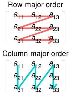
ndarray memory layout
 X = np.ones([3,5],order='F')
 # OR...
 The memory layout (C or Fortran # Y is C-ordered by default
 order) can be set: Y = np.ones([3,5])
  This can be important when dealing with # Z is a F-ordered copy of Y
 external libraries written in R, Matlab, etc. Z = np.asfortranarray(Y)

 Row-major order: C, C++, Java, C#,
 and others

 Column-major order: Fortran, R,
 Matlab, and others

 https://en.wikipedia.org/wiki/Row-_and_column-major_order

ndarray indexing oneD = np.array([1,2,3,4])
 twoD = oneD.reshape([2,2])

 twoD 
 ndarray indexing is similar to array([[1, 2],
 [3, 4]])
 Python lists, strings, tuples, etc.
 # index from 0
 oneD[0]  1
 Index with integers, starting from oneD[3]  4
 zero.
 # -index starts from the end
 oneD[-1]  4
 oneD[-2]  3
 Indexing N-dimensional arrays,
 just use commas: # For multiple dimensions use a comma
 # matrix[row,column]
 array[i,j,k,l] = 42 twoD[0,0]  1
 twoD[1,0]  3

y = np.arange(50,300,50)
 ndarray slicing y --> array([ 50, 100, 150, 200, 250])

 Syntax for each dimension (same
 y[0:3] --> array([ 50, 100, 150])
 rules as lists): y[-1:-3:-1] --> array([250, 200])
  start:end:step
  start:  from starting index to end
  :end  start from 0 to end (exclusive of x = np.arange(10,130,10).reshape(4,3)
 end) x --> array([[ 10, 20, 30],
 [ 40, 50, 60],
  :  all elements.
 [ 70, 80, 90],
 Slicing an ndarray does not make [100, 110, 120]])
 a copy, it creates a view to the
 # 1-D returned!
 original data. x[:,0] --> array([ 10, 40, 70, 100])
 Slicing a Python list creates a # 2-D returned!
 x[2:4,1:3] --> array([[ 80, 90],
 copy. [110, 120]])

 Look at the file slicing.py

ndarray math
 a = np.array([1,2,3,4])
 By default operators work b = np.array([4,5,6,7])
 element-by-element c = a / b
 # c is an ndarray
 print(type(c))  
 These are executed in
 compiled C code. a * b  array([ 4, 10, 18, 28])
 a + b  array([ 5, 7, 9, 11])
 a - b  array([-3, -3, -3, -3])
 a / b  array([0.25, 0.4, 0.5, 0.57142857])
 -2 * a + b  array([ 2, 1, 0, -1])

 Vectors are applied
 a = np.array([2,2,2,2])
 row-by-row to matrices
 c = np.array([[1,2,3,4],
 [4,5,6,7],
 [1,1,1,1],
 The length of the vector [2,2,2,2]])  array([[1, 2, 3, 4],
 must match the width of [4, 5, 6, 7],
 [1, 1, 1, 1],
 the row. [2, 2, 2, 2]])
 a + c  array([[3, 4, 5, 6],
 [6, 7, 8, 9],
 [3, 3, 3, 3],
 [4, 4, 4, 4]])

Linear algebra multiplication
 a = [[1, 0], [0, 1]]
 b = np.array([[4, 1], [2, 2]])
 Vector/matrix multiplication can np.dot(a, b)  array([[4, 1],
 [2, 2]])
 be done using the dot() and
 cross() functions.

 There are many other linear x = [1, 2, 3]
 y = [4, 5, 6]
 algebra routines! np.cross(x, y)  array([-3, 6, -3])

 https://docs.scipy.org/doc/numpy/reference/routines.linalg.html

NumPy I/O
 When reading files you can use standard Python, use lists, allocate
 ndarrays and fill them.

 Or use any of NumPy’s I/O routines that will directly generate ndarrays.

 The best way depends on the structure of your data.

 If dealing with structured numeric data (tables of numbers, etc.) NumPy is
 easier and faster.
 Docs: https://docs.scipy.org/doc/numpy/reference/routines.io.html

A numpy and matplotlib example

 numpy_matplotlib_fft.py is a short example on using numpy and matplotlib
 together.

 Open numpy_matplotlib_fft.py

 Let’s walk through this…

Numpy docs

 As numpy is a large library we can only cover the basic usage here

 Let’s look that the official docs:
https://docs.scipy.org/doc/numpy/reference/index.html

 As an example, computing an average:
https://docs.scipy.org/doc/numpy/reference/generated/numpy.mean.html#numpy.mean

Some numpy file reading options
 numpy.save # save .npy
 numpy.savez # save .npz
 .npz and .npy file formats (cross-platform
 # ditto, with compression
 compatible) : numpy.savez_compressed
  .npy files store a single NumPY variable in a binary
 format. numpy.load # load .npy
  .npz files store multiple NumPy Variables in a file. numpy.loadz # load .npz

 h5py is a library that reads HDF5 files into
 ndarrays
 Tutorial:
 https://docs.scipy.org/doc/nu
 The I/O routines allow for flexible reading from
 mpy/user/basics.io.html
 a variety of text file formats

Outline
 The numpy library

 Libraries: scipy and opencv

 When numpy / scipy isn’t fast enough

• physical constants and conversion factors
SciPy • hierarchical clustering, vector quantization, K-
 means
 • Discrete Fourier Transform algorithms
 SciPy builds on top of • numerical integration routines
 NumPy. • interpolation tools
 • data input and output
 • Python wrappers to external libraries
 Ndarrays are the basic data • linear algebra routines
 structure used. • miscellaneous utilities (e.g. image reading/writing)
 • various functions for multi-dimensional image
 processing
 Libraries are provided for: • optimization algorithms including linear
 programming
 • signal processing tools
 Comparable to Matlab • sparse matrix and related algorithms
 toolboxes. • KD-trees, nearest neighbors, distance functions
 • special functions
 • statistical functions

scipy.io
 I/O routines support a wide variety of file formats:
 Software Format Read? Write?
 name
 Matlab .mat Yes Yes
 IDL .sav Yes No
 Matrix Market .mm Yes Yes
 Netcdf .nc Yes Yes
 Harwell-Boeing .hb Yes Yes
 (sparse matrices)
 Unformatted Fortran files .anything Yes Yes
 Wav (sound) .wav Yes Yes
 Arff .arff Yes No
 (Attribute-Relation File Format)

 
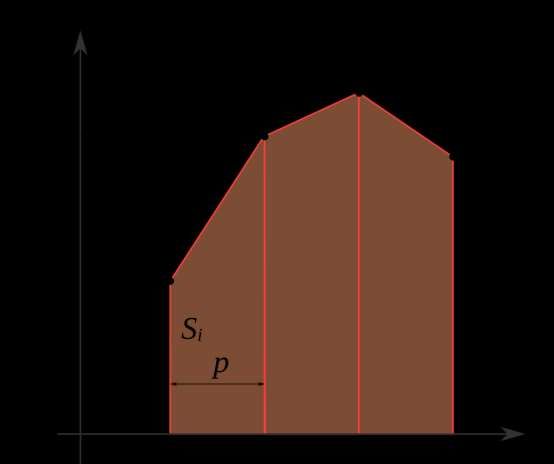
 න 
scipy.integrate 

 Routines for numerical integration

 With a function object:
  quad: uses the Fortran QUADPACK algorithm
  romberg: Romberg algorithm
  newton_cotes: Newton-Cotes algorithm
  And more…

 With fixed samples:
  trapz: Trapezoidal rule
  simps: Simpson’s rule

 https://en.wikipedia.org/wiki/Trapezoidal_rule

scipy.integrate
 Open integrate.py and let’s look at examples of fixed samples and
 function object integration.

 trapz docs:
 https://docs.scipy.org/doc/scipy/reference/generated/scipy.integrate.tra
 pz.html#scipy.integrate.trapz

 romberg docs. Passing functions as arguments is a common pattern in
 SciPy:
 https://docs.scipy.org/doc/scipy/reference/generated/scipy.integrate.ro
 mberg.html#scipy.integrate.romberg

Using SciPy
 Think about your code and what sort of algorithms you’re using:
  Integration, linear algebra, image processing, etc.

 See if an appropriate algorithm exists in SciPy before trying to write
 your own.

 Read the docs – many functions have large numbers of optional
 arguments.

 Understand the algorithms!

OpenCV
 • Image Processing
 • Image file reading and writing
 The Open Source Computer
 • Video I/O
 Vision Library • High-level GUI
 • Video Analysis
 • Camera Calibration and 3D Reconstruction
 Highly optimized and mature C++ • 2D Features Framework
 library usable from C++, Java, and • Object Detection
 Python. • Deep Neural Network module
 • Machine Learning
 • Clustering and Search in Multi-Dimensional Spaces
 Cross platform: Windows, Linux, • Computational Photography
 Mac OSX, iOS, Android • Image stitching

OpenCV vs SciPy

 For imaging-related operations and many linear algebra functions there is a
 lot of overlap between these two libraries.

 OpenCV is frequently faster, sometimes significantly so.

 The OpenCV Python API uses NumPy ndarrays, making OpenCV algorithms
 compatible with SciPy and other libraries.

OpenCV vs SciPy
 A simple benchmark: Gaussian and median
 filtering a 1024x671 pixel image of the CAS
 building.
 Gaussian: radius 5, median: radius 9. See: image_bench.py
 Timing: 2.4 GHz Xeon E5-2680 (Sandybridge)

 Operation Function Time (msec) OpenCV speedup

 scipy.ndimage.gaussian_filter 85.7
 Gaussian 3.7x
 cv2.GaussianBlur 23.2

 scipy.ndimage.median_filter 1,780
 Median 22.5x
 cv2.medianBlur 79.2

When NumPy and SciPy aren’t fast enough

 Auto-compile your Python code with the numba and numexpr libraries

 Use the Intel Python distribution

 Re-code critical paths with Cython

 Combine your own C++ or Fortran code with SWIG and call from Python

numba

 The numba library can translate portions of your Python code and compile
 it into machine code on demand.

 Achieves a significant speedup compared with regular Python.

 Compatible with numpy ndarrays.

 Can generate code to execute automatically on GPUs.

numba from numba import jit

 The @jit decorator is used to # This will get compiled when it's
 indicate which functions are first executed
 @jit
 compiled.
 def average(x, y, z):
 Options: return (x + y + z) / 3.0
  GPU code generation
  Parallelization
  Caching of compiled code # With type information this one gets
 # compiled when the file is read.
 @jit (float64(float64,float64,float64))
 Can produce faster array code def average_eager(x, y, z):
 than pure NumPy statements. return (x + y + z) / 3.0

numexpr
 import numpy as np
 Another acceleration library for import numexpr as ne
 Python.
 a = np.arange(10)
 b = np.arange(0, 20, 2)
 Useful for speeding up specific
 ndarray expressions. # Plain NumPy
  Typically 2-4x faster than plain NumPy c = 2 * a + 3 * b

 Code needs to be edited to move # Numexpr
 ndarray expressions into the d = ne.evaluate("2*a+3*b")
 numexpr.evaluate function:

Intel Python

 Intel now releases a customized build of Python 2.7 and 3.6 based on
 their optimized libraries.

 Can be installed stand-alone or inside of Anaconda:
 https://software.intel.com/en-us/distribution-for-python

 Available on the SCC: module avail python2-intel (or python3-intel)

Intel Python

 In RCS testing on various projects the Intel Python build is always at least
 as fast as the regular Python and Anaconda modules on the SCC.
  In one case involving processing several GB’s of XML code it was 20x faster!

 Easy to try: change environments in Anaconda or load the SCC module.

 Can use the Intel Thread Building Blocks library to improve multithreaded
 Python programs:

 python -m tbb parallel_script.py

Cython

 Cython is a superset of the Python language.

 The additional syntax allows for C code to be auto-generated and
 compiled from Python code.

 This can make mixing Python, Cython, and C code (or libraries) very
 straightforward.

 A mature library that is widely used.

You feel the need for speed…
 Auto-compilation systems like numba, numexpr, and Cython:
  all provide access to higher speed code
  minimal to significant code changes
  You’re still working in Python or Python-like code
  Faster than NumPy which is also much faster than plain Python for numeric calculation

 For the fastest implementation of algorithms, optimized and well-written C,
 C++, and Fortran codes cannot be beat
  In most cases.

 You can write your own compiled code and link it into Python via Cython
 or the SWIG tool. Contact RCS for help!