Phonetic Word Embeddings - Rahul Sharma , Kunal Dhawan , Balakrishna Pailla
←
→
Page content transcription
If your browser does not render page correctly, please read the page content below
Phonetic Word Embeddings

                                                                       Rahul Sharma∗, Kunal Dhawan∗, Balakrishna Pailla
                                                                                      Reliance Jio AI-CoE

                                                                      Abstract                  phonetic signature of the words. This methodology
                                                                                                places two words in the embedding space closer
                                             This work presents a novel methodology for
                                             calculating the phonetic similarity between
                                                                                                if they sound similar. Such an embedding finds
                                             words taking motivation from the human per-        application in various tasks like keyword detection
arXiv:2109.14796v1 [cs.CL] 30 Sep 2021

                                             ception of sounds. This metric is employed         (Sacchi et al., 2019) and poetry generation (Parrish,
                                             to learn a continuous vector embedding space       2017). In (Parrish, 2017), the author clearly defines
                                             that groups similar sounding words together        the concept of phonetic similarity:
                                             and can be used for various downstream com-
                                             putational phonology tasks. The efficacy of             Alliteration, assonance, consonance and
                                             the method is presented for two different               rhyme are all figures of speech deployed
                                             languages (English, Hindi) and performance              in literary writing in order to create pat-
                                             gains over previous reported works are dis-             terns of sound, whether to focus attention
                                             cussed on established tests for predicting pho-
                                                                                                     or to evoke synthetic associations. These
                                             netic similarity. To address limited benchmark-
                                             ing mechanisms in this field, we also intro-            figures are all essentially techniques for
                                             duce a heterographic pun dataset based eval-            introducing phonetic similarity into a
                                             uation methodology to compare the effective-            text, whether that similarity is local to a
                                             ness of acoustic similarity algorithms. Further,        single word, or distributed across larger
                                             a visualization of the embedding space is pre-          stretches of text.
                                             sented with a discussion on the various pos-
                                             sible use-cases of this novel algorithm. An        (Parrish, 2017) introduces a strategy of using pho-
                                             open-source implementation is also shared to       netic feature bi-grams for computing vector repre-
                                             aid reproducibility and enable adoption in re-     sentation of a word. This combines the notion that
                                             lated tasks.
                                                                                                phonemes can be differentiated from each other
                                         1   Introduction                                       using a limited set of properties (Distinctive fea-
                                                                                                ture theory (Chomsky and Halle, 1968)) and that
                                         Word embeddings have become an indispensable           articulation of speech is not discrete, thus acoustic
                                         element of any Natural Language Processing (NLP)       features are affected by the phonemes preceding
                                         pipeline. This technique transforms written words      and following it (Browman and Goldstein, 1992).
                                         to a higher dimensional subspace usually on the        We build upon these ideas and further try to incor-
                                         basis of semantics, providing algorithms the ben-      porate the way in which humans perceive speech
                                         efits of vector spaces like addition and projection    and acoustic similarity. This ideology led us to
                                         while dealing with words. They are currently be-       propose a novel phonetic similarity metric which
                                         ing used for diverse tasks like question answering     is presented in detail in this paper.
                                         systems (Zhou et al., 2015), sentiment analysis (Gi-      The contributions of this paper are as follows:
                                         atsoglou et al., 2017), speech recognition (Bengio     (i) algorithm for similarity between two phonemes
                                         and Heigold, 2014), and many more. These embed-        based on well defined phonetic features; (ii) an
                                         ding spaces are usually learned on the basis of the    edit distance (Wagner and Fischer, 1974) based
                                         meaning of the word, as highlighted in the seminal     approach for computing the acoustic similarity be-
                                         work of word2vec (Mikolov et al., 2013).               tween two words; (iii) a novel non-diagonal penalty
                                            In this work, we explored a parallel ideology for   for matching the phonetic sequence of two words;
                                         learning word embedding spaces - based on the          (iv) a novel end of the word phone weightage factor
                                             ∗
                                                 equal contribution                             that captures the perceptual sound similarity ability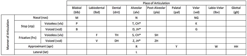
of humans; and (v) results are reported for two lan- formed with different standard words and compari-
guages, English and Hindi. The results for English son words. Vitz and Winkler compared the elicited
comfortably outperform previous best-reported re- scores to the results from their own procedure for
sults and this is the first instance that such results determining phonetic similarity (termed “Predicted
are reported for Hindi, to the best of our knowl- Phonemic Distance,” shortened here as PPD). (Par-
edge. rish, 2017) proposes a novel technique of using
The remainder of the paper is organized as phonetic feature bi-grams for computing vector rep-
follows- We present a literature review in Section 2, resentation of a word. The technique was shown to
Section 3 discusses the proposed approach in de- perform better than (Vitz and Winkler, 1973)’s PPD
tail, the experiments performed and results are dis- approach in some cases. The author works with
cussed in Section 4 and finally the work is con- version 0.7b of the CMU Pronouncing Dictionary
cluded in Section 5. (Carnegie Mellon Speech Group, 2014), which con-
The source code, for the proposed sists of 133852 entries, appends a token ’BEG’ to
method alongside experiments, has been beginning & ’END’ to the end of the phonetic tran-
released publicly and can be accessed at scription of all the words and calculates interleaved
https://github.com/rahulsrma26/phonetic-word- feature bi-grams for each of them. Using the fact
embedding that there can be 949 unique interleaved feature bi-
grams across the entire dataset, the author represent
2 Related work the features extracted for all the words as a matrix
of size 133852 (number of words in the dictionary)
In literature, there have been multiple works that × 949 (number of unique features). PCA is applied
employ phonetic similarity techniques for various to the above matrix to get 50 dimensional embed-
downstream tasks like studying language similari- ding for each of the words in the dataset, which we
ties, diachronic language change, comparing pho- refer to as PSSVec in this paper, short for Poetic
netic similarity with perceptual similarity, and so Sound Similarity Vector. To capture the similarity
on. This diverse usage acts as a strong motiva- of words regardless of the ordering of phonemes,
tion for us to come up with a more accurate and the author further computes the features for the re-
robust phonetic similarity-based word embedding verse order of the phonemes and appends that to
algorithm. the original feature of the word. Thus, a drawback
(Bradlow et al., 2010) explores methods repre- of this approach is that embedding is not dependent
senting languages in a perceptual similarity space of the position of the phoneme in the word, for
based on their overall phonetic similarity. It aims to example, the embedding for phoneme sequences
use this phonetic and phonological likeness of any ’AY P N OW’ and ’OW N P AY’ would turn out
two languages to study patterns of cross-language to be same, which is counter-intuitive as they don’t
and second-language speech perception and pro- sound similar. Hence, we postulate that the posi-
duction. It is important to note that their focus is not tion of phonemes also plays a major role for two
on words in a language but rather the usage of the words to sound similar (and thus be closer to each
similarity space to study the relationship between other in the embedding space) and we address this
languages. (Mielke, 2012) talks about quantifying issue in our proposed similarity algorithm.
phonetic similarity and how phonological notions
of similarity are different from articulatory, acous- 3 Proposed Approach
tic, and perceptual similarity. The proposed metric,
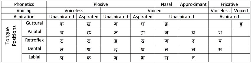
which is based on phonetic features, was compared It has been well established by linguists that some
with measures for phonological similarity, which phonemes are more similar than others depend-
are calculated by counting the co-occurrences of ing upon the variations in articulatory positions
pairs of sounds in the same phonologically active involved while producing them (Chomsky and
classes. In the experiments conducted by (Vitz and Halle, 1968), and these variations are captured
Winkler, 1973), small groups of L1 American En- by phoneme features. Based on these features
glish speakers were asked to score the phonetic phonemes can be categorized into groups. Our
similarity of a “standard” word with a list of com- method assumes that each phoneme can be mapped
parison words on a scale from 0 (no similarity) to 4 to a set of corresponding phonetic features. For
(extremely similar). Several experiments were per- English, we use the mapping suggested in the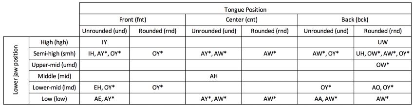
Table 1: Complete feature description for English consonants (* denotes multiple occupancy of the given phoneme)

 Table 2: Complete feature description for English vowels (* denotes multiple occupancy of the given phoneme)

                          Table 3: Complete feature description for Hindi consonants

                            Table 4: Complete feature description for Hindi vowels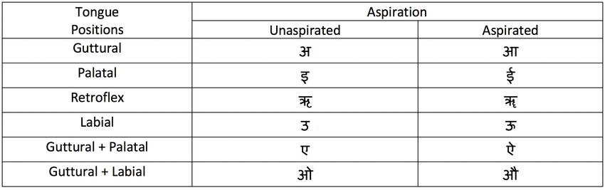
specification for X-SAMPA (Kirshenbaum, 2001), idea.
adapted to the Arpabet transcription scheme. The
Sv ((Pa1 , Pa2 ), (Pb1 , Pb2 )) =
mapping of English phonemes to features is shown p
in table 1 and 2.
S((Pa1 , Pa2 ), (Pb1 , Pb2 )),
After Mandarin, Spanish and English, Hindi is if Pa2 is a vowel and Pa2 = Pb2
the most natively spoken language in the world,
almost spoken by 260 million people according to
S((P , P ), (P , P ))2 , otherwise
a1 a2 b1 b2
(Ethnologue, 2014). For Hindi, we use the mapping
(4)
suggested by (Malviya et al., 2016) and added some
of the missing ones using IPA phonetic features Here, Sv is the vowel-weighted similarity for the
(Mortensen et al., 2016). The mapping of Hindi bi-grams (Pa1 , Pa2 ) and (Pb1 , Pb2 ).
phonemes to features used by us is shown in tables
3 and 4. 3.2 Word Similarity
We are proposing a novel method to compare words
3.1 Phoneme Similarity that take the phoneme similarity as well as their
sequence into account. The symmetric similarity
The phonetic distance (Similarity) S between a pair distance between word a, given as the phoneme
of phonemes Pa and Pb is measured by using the sequence a1 , a2 , a3 . . . an , and word b, given as
feature set of two phonemes and computing Jaccard the phoneme sequence b1 , b2 , b3 . . . bm is given by
similarity. dnm , defined by the recurrence:
|F (Pa ) ∩ F (Pb )| d1,1 = S(a1 , b1 )
S(Pa , Pb ) = (1)
|F (Pa ) ∪ F (Pb )|
di,1 = di−1,1 + S(ai , b1 ) for 2 ≤ i ≤ n
Here, F (P ) is the set of all the feature of phone
P . For example, F (R) = {apr, alv} (from table d1,j = d1,j−1 + S(a1 , bj ) for 2 ≤ j ≤ m
1). We can extend this logic to bi-grams as well.
To compute the feature set of bi-gram (Pa1 , Pa2 ),
we will just take the union of the features for both
of the phones.
S(ai , bj ) + di−1,j−1 , if S(ai , bj ) = 1
S(a , b )/p
i j (
di,j =
F (Pa1 , Pa2 ) = F (Pa1 ) ∪ F (Pa2 ) (2) di−1,j , otherwise
+min d
i,j−1
And Similarity S between pairs of bi-grams for 2 ≤ i ≤ n, 2 ≤ j ≤ m
(Pa1 , Pa2 ) and (Pb1 , Pb2 ), can be calculated as: (5)
Here, p is the non-diagonal penalty. As we are
calculating scores for all possible paths, this allows
S((Pa1 , Pa2 ), (Pb1 , Pb2 )) = us to discourage the algorithm from taking con-
|F (Pa1 , Pa2 ) ∩ F (Pb1 , Pb2 )| voluted non-diagonal paths, which will otherwise
|F (Pa1 , Pa2 ) ∪ F (Pb1 , Pb2 )| amass better scores as they are longer. The word
(3) similarity WS between the words a and b can be
calculated as:
Vowels in speech are in general longer than con- WS (a, b) = dn,m /max(n, m) (6)
sonants (Umeda, 1975) (Umeda, 1977) and further
the perception of similarity is heavily dependent By setting non-diagonal penalty p ≥ 2, we can
upon vowels (Raphael, 1972). This is the reason ensure that word similarity WS will be in the range
that if two bi-grams are ending with the same vowel 0 ≤ WS ≤ 1.
then they sound almost the same despite them start- Further, the score can be calculate for a bi-
ing with different consonants. gram sequence instead of a uni-gram sequence
We can weight our similarity score to reflect this by using equation 3. In case of bi-grams, we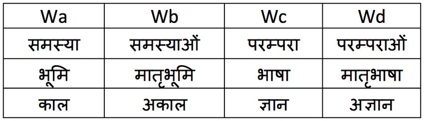
inserte two new tokens: ’BEG’ in the begin-                4     Experiments and Results
ning and ’END’ in the end of the phoneme se-
                                                           4.1    Experiments
quence. For word a, defined by the original se-
quence a1 , a2 , a3 . . . an , the bi-gram sequence will   We implemented the memoized version of the
be (BEG, a1 ), (a1 , a2 ), (a2 , a3 ), (a3 , a4 ) . . .    algorithm using dynamic programming. Given
(an−1 , an ), (an , EN D). Here, ’BEG’ and ’END’           two words a and b with phoneme sequences
are the dummy phones which are mapped to the               a = a1 , a2 , a3 . . . an and b = b1 , b2 , b3 . . . bm , the
single dummy phonetic features ’beg’ and ’end’             complexity of the algorithm is O(n.m). The
respectively.                                              algorithm is implemented in Python and CMU
   We can also utilize the benefits of vowel weight        Pronouncing Dictionary 0.7b (Carnegie Mellon
concept that we established in equation 4. The only        Speech Group, 2014) is used to obtain the phoneme
change required in the equation 3.2 is to use Sv           sequence for a given word.
instead of S in the calculation of symmetric simi-            As described below, for comparison of our pro-
larity distance dn,m . We denote the word similarity       posed approach to existing work, we calculated
obtained via this method as WSV (vowel weighted            the correlation between human scores to the scores
word similarity) in this paper.                            given by PSSVec and our method for all the stan-
                                                           dard words as outlined in (Vitz and Winkler, 1973).
3.3   Embedding Calculation                                   First we use our algorithm WS on uni-grams
Using the algorithm mentioned in the previous sec-         and then bi-grams. For bi-grams we have used 3
tion, we can obtain similarities between any two           variations: one without non-diagonal penalty (i.e.
words, as long as we have their phonemic break-            p = 1), one with p = 2.5 and one with the vowel
down. In this section, we highlight the approach           weights (WSV ). We compared the correlation be-
followed to build an embedding space for the words.        tween methods and the human survey results (Vitz
Word embeddings offer many advantages like faster          and Winkler, 1973). We scaled the human survey
computation and independent handling in addition           results from 0-4 to 0-1. As seen in figure 1, giv-
to the other benefits of vector spaces like addition,      ing preference to the matching elements by setting
subtraction, and projection.                               p = 2.5 increased the score. Effect of the non-
   For a k word dictionary, we can obtain the sim-         diagonal penalty p can be seen in figure 3. This
ilarity matrix M ∈ Rk∗k by computing the word              also shows that giving higher weights to similar
similarity between all the pairs of word.                  ending vowels further increased the performance.
                                                              After that, we compared our method (bi-gram
            Mi,j = WSV (wordi , wordj )             (7)    with WSV and p = 2.5) with the existing work.
                                                           As we can see from the figure 2, our method out
Since this similarity matrix M will be a symmetric         performs the existing work in all 4 cases.
non-negative matrix, one can use Non-negative Ma-
                                                           4.2    Embedding Space Calculation
trix Factorization (Yang et al., 2008) or a similar
technique to obtain the d dimension word embed-            As the vowel weighted bi-gram based method WSV
ding V ∈ Rk∗d . Using Stochastic Gradient De-              with non-diagonal penalty p = 2.5 gave us the best
scent(SGD) (Koren et al., 2009) based method we            performance, we use this to learn embeddings by
can learn the embedding matrix V by minimizing:            solving equation 8. Tensorflow v2.1 (Abadi et al.,
                                                           2016) was used for implementation of our matrix
                   ||M − V.V T ||2                  (8)    factorization code..
                                                              As python implementation is slow, we have also
   We choose SGD based method as matrix fac-               implemented our algorithm in C++ and used it in
torization and other such techniques become in-            Tensorflow (for on-fly batch calculation) by expos-
efficient due to the memory requirements as the            ing it as a python module using Cython (Seljebotn,
number of words k increases. For example to fit            2009). In single-thread comparison we got an av-
the similarity matrix M in memory for k words              erage speed-up around 300x from the C++ imple-
the space required will be in the order of O(k 2 ).        mentation over the Python implementation. The
But using SGD based method we don’t need to                implementation benefits from the compiler intrin-
pre-calculate the M matrix, we can just calculate          sics for bit-count (Muła et al., 2018) which speedup
the required values by using equation 7 on the fly.        the Jaccard similarity computation. The results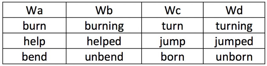
Figure 2: Correlation of existing work and our method
Figure 1: Correlation of proposed methods with Hu-      with Human Survey
man Survey

   Figure 3: Effect of the penalty on correlation       Figure 4: Correlation of embeddings with Human Sur-
                                                        vey

               Figure 5: Visualizing the acoustic embedding vectors of selected English words
Figure 6: Visualizing the acoustic embedding vectors of selected Hindi words
were obtained on Intel(R) Xeon(R) CPU E5-2690
v4 @ 2.60GHz 440GB RAM server machine run-
ning on Ubuntu 18.04. To compare the running
performance, we use the time taken to compute the
similarity between a given word to every word in
Table 5: Sound analogies for English
the dictionary. The experiments were repeated 5
times and their average was taken for the studies.
Similar to PSSVec we also used 50 dimensional
embeddings for a fair comparison. The English em-
beddings are trained on 133859 words from CMU
0.7b dictionary (Carnegie Mellon Speech Group,
2014). Figure 4 shows the comparison between Table 6: Sound analogies for Hindi
PSSVec and our embeddings.
To aid visual understanding of this embedding
For Hindi language, we use (Kunchukuttan,
space, we selected a few words each from En-
2020) dataset and train on 22877 words.
glish & Hindi languages and projected their embed-
We can also perform sound analogies (which dings to a 2-dimensional space using t-distributed
reveal the phonetic relationships between words) stochastic neighbor embedding (Maaten and Hin-
on our obtained word embeddings using vector ton, 2008). The projected vectors are presented
arithmetic to showcase the efficacy of the learned as a 2D plot in figure 5 for English and figure 6
embedding space. Let’s assume that V (W ) repre- for Hindi. We clearly note that similar sounding
sents the learned embedding vector for the word W . words occur together in the plot, hence validating
If Wa is related to Wb via the same relation with our hypothesis that our proposed embedding space
which Wc is related to Wd (Wa : Wb :: Wc : Wd ), is able to capture the phonetic similarity of words.
given the embedding of words Wa , Wb , Wc , we can
obtain Wd as: 4.3 Pun Based Evaluation
A pun is a form of wordplay which exploits the dif-
Wd = N (V (Wb ) − V (Wa ) + V (Wc )) (9) ferent possible meanings of a word or the fact that
there are words that sound alike but have different
where function N (v) returns the nearest word meanings, for an intended humorous or rhetorical
from the vector v in the learnt embedding space. effect (Miller et al., 2017). The first category where
The results for some pairs are documented in the a pun exploits the different possible meanings of
following tables: a word is called Homographic pun and the secondcategory that banks on similar sounding words is with smaller variance and higher mean as compared
called Heterographic pun. Following is an example to PSSVec embeddings.
of a Heterographic pun:
I Renamed my iPod The Titanic,
so when I plug it in, it says
“The Titanic is syncing.”
Heterographic puns are based on similar sound-
ing words and thus act as a perfect benchmarking
dataset for acoustic embedding algorithms. For
showing the efficacy of our approach, we have used
the 3rd subtask (heterographic pun detection) of
the SemEval-2017 Task 7 dataset (Miller et al.,
2017). This test set contains 1098 hetrographic
puns word pairs like syncing and sinking. After Figure 7: Cosine similarity distribution comparison
taking all word pairs that are present in the CMU
Pronouncing Dictionary (Carnegie Mellon Speech
Group, 2014) and removing duplicate entries, we 5 Conclusion
are left with 778 word-pairs. Ideally, for a good
acoustic embedding algorithm, we would expect In this work, we propose a method to obtain the sim-
the distribution of cosine similarity of these word ilarity between a pair of words given their phoneme
pairs to be a sharp Gaussian with values → 1. sequence and a phonetic features mapping for the
To further intuitively highlight the efficacy of language. Overcoming the short-coming of pre-
our approach, for the 778 word-pairs we present in vious embedding based solutions, our algorithm
table 7 the difference of the cosine similarity scores can also be used to compare the similarity of new
obtained from our algorithm and PSSVec (sorted by words coming on the fly, even if they are not seen in
the difference). As we can see, though the words the training data. Further, since embeddings have
mutter and mother are relatively similarly sounding, proven helpful in various cases, we also present
PSSVec assigns a negative similarity. In compari- a word embedding algorithm utilizing our similar-
son, our method is more robust, correctly capturing ity metric. Our embeddings are shown to perform
the acoustic similarity between words. better than previously reported results in the litera-
ture. We claim that our approach is generic and can
Table 7: Difference of scores be extended to any language for which phoneme
sequences can be obtained for all its words. To
Word1 Word2 PSSVec Ours Diff showcase this, results are presented for 2 languages
- English and Hindi.
mutter mother -0.0123 0.8993 0.9117
loin learn -0.0885 0.8119 0.9005 Going forward, we wish to apply our approach to
truffle trouble 0.1365 0.9629 0.8264 more Indian languages, utilizing the fact that there
soul sell 0.0738 0.7642 0.6903 is no sophisticated grapheme-to-phoneme conver-
sion required in most of them as the majority of
sole sell 0.0738 0.7605 0.6866
Indian languages have orthographies with a high
... ... ... ... ...
grapheme-to-phoneme and phoneme-to-grapheme
eight eat 0.7196 0.4352 -0.2844
correspondence. The approach becomes more valu-
allege ledge 0.7149 0.4172 -0.2976
able for Hindi and other Indian languages as there
ache egg 0.7734 0.4580 -0.3154
is very less work done for them and adaptation of
engels angle 0.8318 0.4986 -0.3331
a generic framework allows for diversity and in-
bullion bull 0.7814 0.4128 -0.3685 clusion. We also want to take advantage of this
similarity measure and create a word-based speech
Figure 7 shows the density distribution of the recognition system that can be useful for various
cosine similarity between the test word-pairs for tasks like limited vocabulary ASR, keyword spot-
our proposed algorithm and PSSVec. It is observed ting, and wake-word detection.
that our distribution closely resembles a Gaussian,References Tomas Mikolov, Ilya Sutskever, Kai Chen, Greg S Cor-
rado, and Jeff Dean. 2013. Distributed representa-
Martín Abadi, Ashish Agarwal, Paul Barham, Eugene tions of words and phrases and their compositional-
Brevdo, Zhifeng Chen, Craig Citro, Greg S Corrado, ity. In Advances in neural information processing
Andy Davis, Jeffrey Dean, Matthieu Devin, et al. systems, pages 3111–3119.
2016. Tensorflow: Large-scale machine learning on
heterogeneous distributed systems. arXiv preprint Tristan Miller, Christian F Hempelmann, and Iryna
arXiv:1603.04467. Gurevych. 2017. Semeval-2017 task 7: Detection
and interpretation of english puns. In Proceedings of
Samy Bengio and Georg Heigold. 2014. Word embed- the 11th International Workshop on Semantic Evalu-
dings for speech recognition. ation (SemEval-2017), pages 58–68.
Ann Bradlow, Cynthia Clopper, Rajka Smiljanic, and David R Mortensen, Patrick Littell, Akash Bharadwaj,
Mary Ann Walter. 2010. A perceptual phonetic simi- Kartik Goyal, Chris Dyer, and Lori Levin. 2016.
larity space for languages: Evidence from five native Panphon: A resource for mapping ipa segments to
language listener groups. Speech Communication, articulatory feature vectors. In Proceedings of COL-
52(11-12):930–942. ING 2016, the 26th International Conference on
Computational Linguistics: Technical Papers, pages
Catherine P Browman and Louis Goldstein. 1992. Ar- 3475–3484.
ticulatory phonology: An overview. Phonetica,
49(3-4):155–180. Wojciech Muła, Nathan Kurz, and Daniel Lemire.
2018. Faster population counts using avx2 instruc-
Carnegie Mellon Speech Group. 2014. The CMU Pro- tions. The Computer Journal, 61(1):111–120.
nouncing Dictionary 0.7b.
Allison Parrish. 2017. Poetic sound similarity vec-
Noam Chomsky and Morris Halle. 1968. The sound tors using phonetic features. In Thirteenth Artificial
pattern of english. Intelligence and Interactive Digital Entertainment
Conference.
Ethnologue. 2014. Most Widely Spoken Languages in
the World. Lawrence J Raphael. 1972. Preceding vowel duration
as a cue to the perception of the voicing character-
Maria Giatsoglou, Manolis G Vozalis, Konstantinos istic of word-final consonants in american english.
Diamantaras, Athena Vakali, George Sarigiannidis, The Journal of the Acoustical Society of America,
and Konstantinos Ch Chatzisavvas. 2017. Sentiment 51(4B):1296–1303.
analysis leveraging emotions and word embeddings.
Expert Systems with Applications, 69:214–224. Niccolo Sacchi, Alexandre Nanchen, Martin Jaggi, and
Milos Cernak. 2019. Open-vocabulary keyword
Evan Kirshenbaum. 2001. Represent- spotting with audio and text embeddings. In IN-
ing ipa phonetics in ascii. URL: TERSPEECH 2019-IEEE International Conference
http://www.kirshenbaum.net/IPA/ascii-ipa.pdf on Acoustics, Speech, and Signal Processing.
(unpublished), Hewlett-Packard Laboratories.
Dag Sverre Seljebotn. 2009. Fast numerical computa-
Yehuda Koren, Robert Bell, and Chris Volinsky. 2009. tions with cython. In Proceedings of the 8th Python
Matrix factorization techniques for recommender in Science Conference, volume 37.
systems. Computer, 42(8):30–37.
Noriko Umeda. 1975. Vowel duration in american en-
Anoop Kunchukuttan. 2020. The IndicNLP Library. glish. The Journal of the Acoustical Society of Amer-
https://github.com/anoopkunchukuttan/ ica, 58(2):434–445.
indic_nlp_library/blob/master/docs/
indicnlp.pdf. Noriko Umeda. 1977. Consonant duration in american
english. The Journal of the Acoustical Society of
Laurens van der Maaten and Geoffrey Hinton. 2008. America, 61(3):846–858.
Visualizing data using t-sne. Journal of machine
learning research, 9(Nov):2579–2605. Paul C Vitz and Brenda Spiegel Winkler. 1973. Pre-
dicting the judged “similarity of sound” of english
Shrikant Malviya, Rohit Mishra, and Uma Shanker Ti- words. Journal of Verbal Learning and Verbal Be-
wary. 2016. Structural analysis of hindi phonetics havior, 12(4):373–388.
and a method for extraction of phonetically rich sen-
tences from a very large hindi text corpus. In 2016 Robert A Wagner and Michael J Fischer. 1974. The
Conference of The Oriental Chapter of International string-to-string correction problem. Journal of the
Committee for Coordination and Standardization of ACM (JACM), 21(1):168–173.
Speech Databases and Assessment Techniques (O-
COCOSDA), pages 188–193. IEEE. Jianchao Yang, Shuicheng Yang, Yun Fu, Xuelong Li,
and Thomas Huang. 2008. Non-negative graph em-
Jeff Mielke. 2012. A phonetically based metric of bedding. In 2008 IEEE Conference on Computer
sound similarity. Lingua, 122(2):145–163. Vision and Pattern Recognition, pages 1–8. IEEE.Guangyou Zhou, Tingting He, Jun Zhao, and Po Hu. 2015. Learning continuous word embedding with metadata for question retrieval in community ques- tion answering. In Proceedings of the 53rd Annual Meeting of the Association for Computational Lin- guistics and the 7th International Joint Conference on Natural Language Processing (Volume 1: Long Papers), pages 250–259.
You can also read