CROSS-DOMAIN IMITATION LEARNING VIA OPTIMAL TRANSPORT - OpenReview
←
→
Page content transcription
If your browser does not render page correctly, please read the page content below
Under review as a conference paper at ICLR 2022

C ROSS -D OMAIN I MITATION L EARNING
VIA O PTIMAL T RANSPORT

 Anonymous authors
 Paper under double-blind review

                                                  A BSTRACT

             Cross-domain imitation learning studies how to leverage expert demonstrations of
             one agent to train an imitation agent with a different embodiment or morphology.
             Comparing trajectories and stationary distributions between the expert and imi-
             tation agents is challenging because they live on different systems that may not
             even have the same dimensionality. We propose Gromov-Wasserstein Imitation
             Learning (GWIL), a method for cross-domain imitation that uses the Gromov-
             Wasserstein distance to align and compare states between the different spaces of
             the agents. Our theory formally characterizes the scenarios where GWIL pre-
             serves optimality, revealing its possibilities and limitations. We demonstrate the
             effectiveness of GWIL in non-trivial continuous control domains ranging from
             simple rigid transformation of the expert domain to arbitrary transformation of
             the state-action space. 1

1       I NTRODUCTION

Reinforcement learning (RL) methods have attained impressive results across a number of domains,
e.g., Berner et al. (2019); Kober et al. (2013); Levine et al. (2016); Vinyals et al. (2019). However,
the effectiveness of current RL method is heavily correlated to the quality of the training reward. Yet
for many real-world tasks, designing dense and informative rewards require significant engineering
effort. To alleviate this effort, imitation learning (IL) proposes to learn directly from expert demon-
strations. Most current IL approaches can be applied solely to the simplest setting where the expert
and the agent share the same embodiment and transition dynamics that live in the same state and
action spaces. In particular, these approaches require expert demonstrations from the agent domain.
Therefore, we might reconsider the utility of IL as it seems to only move the problem, from design-
ing informative rewards to providing expert demonstrations, rather than solving it. However, if we
relax the constraining setting of current IL methods, then natural imitation scenarios that genuinely
alleviate engineering effort appear. Indeed, not requiring the same dynamics would enable agents to
imitate humans and robots with different morphologies, hence widely enlarging the applicability of
IL and alleviating the need for in-domain expert demonstrations.
This relaxed setting where the expert demonstrations comes from another domain has emerged as a
budding area with more realistic assumptions (Gupta et al., 2017; Liu et al., 2019; Sermanet et al.,
2018; Kim et al., 2020; Raychaudhuri et al., 2021) that we will refer to as Cross-Domain Imitation
Learning. A common strategy of these works is to learn a mapping between the expert and agent
domains. To do so, they require access to proxy tasks where both the expert and the agent act
optimally in there respective domains. Under some structural assumptions, the learned map enables
to transform a trajectory in the expert domain into the agent domain while preserving the optimality.
Although these methods indeed relax the typical setting of IL, requiring proxy tasks heavily restrict
the applicability of Cross-Domain IL. For example, it rules out imitating an expert never seen before
as well as transferring to a new robot.
In this paper, we relax the assumptions of Cross-Domain IL and propose a benchmark and method
that do not need access to proxy tasks. To do so, we depart from the point of view taken by previous
work and formalize Cross-Domain IL as an optimal transport problem. We propose a method, that
we call Gromov Wasserstein Imitation Learning (GWIL), that uses the Gromov-Wasserstein distance
    1
        Project site with videos: https://sites.google.com/view/gwil/home

                                                         1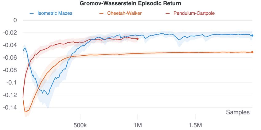
Under review as a conference paper at ICLR 2022

Figure 1: The Gromov-Wasserstein distance enables us to compare the stationary state-action distri-
butions of two agents with different dynamics and state-action spaces. We use it as a pseudo-reward
for cross-domain imitation learning.

Figure 2: Isometric policies (definition 2) have the same pairwise distances within the state-action
space of the stationary distributions. In Euclidean spaces, isometric transformations preserve these
pairwise distances and include rotations, translations, and reflections.

to solve the benchmark. We formally characterize the scenario where GWIL preserves optimality
(theorem 1), revealing the possibilities and limitations. The construction of our proxy rewards to
optimize optimal transport quantities using RL generalizes previous work that assumes uniform
occupancy measures (Dadashi et al., 2020; Papagiannis & Li, 2020) and is of independent interest.
Our experiments show that GWIL learns optimal behaviors with a single demonstration from another
domain without any proxy tasks in non-trivial continuous control settings.

2   R ELATED W ORK

Imitation learning. An early approach to IL is Behavioral Cloning (Pomerleau, 1988; 1991) which
amounts to training a classifier or regressor via supervised learning to replicate the expert’s demon-
stration. Another key approach is Inverse Reinforcement Learning (Ng & Russell, 2000; Abbeel &
Ng, 2004; Abbeel et al., 2010), which aims at learning a reward function under which the observed
demonstration is optimal and can then be used to train a agent via RL. To bypass the need to learn
the expert’s reward function, Ho & Ermon (2016) show that IRL is a dual of an occupancy measure
matching problem and propose an adversarial objective whose optimization approximately recover
the expert’s state-action occupancy measure, and a practical algorithm that uses a generative ad-
versarial network (Goodfellow et al., 2014). While a number of recent work aims at improving this
algorithm relative to the training instability caused by the minimax optimization, Primal Wasserstein
Imitation Learning (PWIL) (Dadashi et al., 2020) and Sinkhorn Imitation Learning (SIL) (Papagian-
nis & Li, 2020) view IL as an optimal transport problem between occupancy measures to completely
eliminate the minimax objective and outperforms adversarial methods in terms of sample efficiency.
Heess et al. (2017); Peng et al. (2018); Zhu et al. (2018); Aytar et al. (2018) scale imitation learn-
ing to complex human-like locomotion and game behavior in non-trivial settings. Our work is an
extension of Dadashi et al. (2020); Papagiannis & Li (2020) from the Wasserstein to the Gromov-
Wasserstein setting. This takes us beyond limitation that the expert and imitator are in the same
domain and into the cross-domain setting between agents that live in different spaces.
Transfer learning across domains and morphologies. Work transferring knowledge between dif-
ferent domains in RL typically learns a mapping between the state and action spaces. Ammar et al.
(2015) use unsupervised manifold alignment to find a linear map between states that have similar
local geometry but assume access to hand-crafted features. More recent work in transfer learning

                                                  2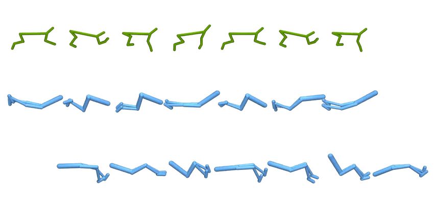
Under review as a conference paper at ICLR 2022
across viewpoint and embodiment mismatch learn a state mapping without handcrafted features but
assume access to paired and time-aligned demonstration from both domains (Gupta et al., 2017; Liu
et al., 2018; Sermanet et al., 2018). Furthermore, Kim et al. (2020); Raychaudhuri et al. (2021)
propose methods to learn a state mapping from unpaired and unaligned tasks. All these methods
require proxy tasks, i.e. a set of pairs of expert demonstrations from both domains, which limit the
applicability of these methods to real-world settings. Stadie et al. (2017) have proposed to combine
adversarial learning and domain confusion to learn a policy in the agent’s domain without proxy
tasks but their method only works in the case of small viewpoint mismatch. Zakka et al. (2021) take
a goal-driven perspective that seeks to imitate task progress rather than match fine-grained structural
details to transfer between physical robots. In contrast, our method does not rely on learning an
explicit cross-domain latent space between the agents, nor does it rely on proxy tasks. The Gromov-
Wasserstein distance enables us to directly compare the different spaces without a shared space. The
existing benchmark tasks we are aware of assume access to a set of demonstrations from both agents
whereas the experiments in our paper only assume access to expert demonstrations.
3 P RELIMINARIES
Metric Markov Decision Process. An infinite-horizon discounted Markov decision Process (MDP)
is a tuple (S, A, R, P, p0 , γ) where S and A are state and action spaces, P : S × A → ∆(S) is the
transition function, R : S × A → R is the reward function, p0 ∈ ∆(S) is the initial state distribution
and γ is the discount factor. We equip MDPs with a distance d : S × A → R+ and call the tuple
(S, A, R, P, p0 , γ, d) a metric MDP.
Gromov-Wasserstein distance. Let (X , dX , µX ) and (Y, dY , µY ) be two metric measure spaces,
where dX and dY are distances, and µX and µY are measures on their respective spaces2 . The
Gromov-Wasserstein distance (Mémoli, 2011) extends the Wasserstein distance from optimal trans-
portation (Villani, 2009) to these spaces and is defined as
X
GW((X , dX , µX ), (Y, dY , µY ))2 = min |dX (x, x0 ) − dY (y, y 0 )|2 ux,y ux0 ,y0 , (1)
u∈U (µX ,µY )
X 2 ×Y 2
where U(µX , µY ) is the set of couplings between the atoms of the measures defined by
X X
U(µX , µY ) = u ∈ RX ×Y ∀x ∈ X , ux,y = µX (x), ∀y ∈ Y, ux,y = µY (y) .
y∈Y x∈X
GW compares the structure of two metric measure spaces by comparing the pairwise distances
within each space to find the best isometry between the spaces. Figure 1 illustrates this distance in
the case of the metric measure spaces (SE × AE , dE , ρπE ) and (SA × AA , dA , ρπA ).
4 C ROSS -D OMAIN I MITATION L EARNING VIA O PTIMAL T RANSPORT
4.1 C OMPARING POLICIES FROM ARBITRARILY DIFFERENT MDP S
For a stationary policy π acting on a metric MDP (S, A, R, P, γ, d), the occupancy measure is:
∞
X
ρπ : S × A → R ρ(s, a) = π(a|s) γ t P (st = s|π).
t=0
We compare policies from arbitrarily different MDPs in terms of their occupancy measures.
Definition 1 (Gromov-Wasserstein distance between policies). Given an expert policy πE and an
agent policy πA acting, respectively, on
ME = (SE , AE , RE , PE , TE , dE ) and MA = (SA , AA , RA , PA , TA , dA ).
We define the Gromov-Wasserstein distance between πE and πA as the Gromov-Wasserstein distance
between the metric measure spaces (SE × AE , dE , ρπE ) and (SA × AA , dA , ρπA ):
GW(π, π 0 ) = GW((SE × AE , dE , ρπE ), (SA × AA , dA , ρπA )). (2)
2
We use discrete spaces for readability but show empirical results in continuous spaces.
3Under review as a conference paper at ICLR 2022
We now define an isometry between policies by comparing the distances between the state-action
spaces and show that GW defines a distance up to an isometry between the policies. Figure 2
illustrates examples of simple isometric policies.
Definition 2 (Isometric policies). Two policies πE and πA are isometric if there exists a bijection
φ : supp[ρπE ] → supp[ρπA ] that satisfies for all (sE , aE ), (sE 0 , aE 0 ) ∈ supp[ρπE ]2 :
dE ((sE , aE ), (sE 0 , aE 0 )) = dA (φ(sE , aE ), φ(sE 0 , aE 0 ))
In other words, φ is an isometry between (supp[ρπE ], dE ) and (supp[ρπA ], dA ).
Proposition 1. GW defines a metric on the collection of all isometry classes of policies.
Proof. By definition 1, GW(πE , πA ) = 0 if and only if GW((SE , dE , ρπE ), (SA , dA , ρπA )) = 0.
By Mémoli (2011, Theorem 5.1), this is true if and only if there is an isometry that maps supp[ρφE ]
to supp[ρφA ]. By definition 2, this is true if and only if πA and πE are isometric. The symmetry and
triangle inequality follow from Mémoli (2011, Theorem 5.1).
The next theorem3 gives a sufficient condition to recover, by minimizing GW, an optimal policy4 in
the agent’s domain up to an isometry.
Theorem 1. Consider two MDPs
ME = (SE , AE , RE , PE , pE , γ) and MA = (SA , AA , RA , PA , pA , γ).
Suppose that there exists four distances dSE , dA S A
E , dA , dA defined on SE , AE , SA and AE respectively,
and two isometries φ : (SE , dSE ) → (SA , dSA ) and ψ : (AE , dSE ) → (AS , dSA ) such that for all
(sE , aE , s0E ) ∈ SE × AE × SE the three following conditions hold:
R(sE , aE ) = RA (φ(sE ), ψ(aE )) (3)
PE sE ,aE (s0E ) = PAφ(sE )ψ(aE ) (φ(s0E )) (4)
pE (sE ) = pA (φ(sE )). (5)
∗ ∗
Consider an optimal policy πE in ME . Suppose that πGW minimizes GW(πE , πGW ) with
dE : (sE , aE ) 7→ dSE (sE ) + dA S A
E (aE ) and dA : (sA , aA ) 7→ dA (sA ) + dA (aA ).
Then πGW is isometric to an optimal policy in MA .
Proof. Consider the occupancy measure ρ∗A : SA × AA → R given by
(sA , aA ) 7→ ρπE∗ (φ−1 (sA ), ψ −1 (aA )).
We first show that ρ∗A is feasible in MA , i.e. there exists a policy πA ∗
acting in MA with occupancy
measure ρ∗A (a). Then we show that πA ∗
is optimal in MA (b) and is isometric to πE ∗
(c). Finally we
∗
show that πGW is isometric to πA , which concludes the proof (d).
(a) Consider sA ∈ SA . By definition of ρ∗A ,
X X X
ρ∗A (sA ) = ρπE∗ (φ−1 (sA ), ψ −1 (aA )) = ρπE∗ (φ−1 (sA ), aE ).
aA ∈AA aA ∈AA aE ∈AE
Since ρπE∗ is feasible in M , it follows from Puterman (2014, Theorem 6.9.1) that
X X
ρπE∗ (φ−1 (sA ), aE ) = pE (φ−1 (sA )) + γ PE sE ,aE (φ−1 (sA )) + ρπE∗ (sE , aE ).
aE ∈AE sE ∈SE ,aE ∈AE
By conditions 4 and 5 and by definition of ρ∗A ,
X
pE (φ−1 (sA )) + γ PE sE ,aE (φ−1 (sA )) + ρπE∗ (sE , aE )
sE ∈SE ,aE ∈AE
X
= pA (sA ) + γ PAφ(sE ),ψ(aE ) (sA ) + ρ∗A (φ(sE ), ψ(aE ))
sE ∈SE ,aE ∈AE
X
= pA (sA ) + γ PAs0A ,aA (sA ) + ρ∗A (s0A , aA ).
s0A ∈SA ,aA ∈AA
3
Our proof is in finite state-action spaces for readability and can be directly extended to infinite spaces.
4
A policy is optimal in the MDP (S, A, R, P, γ, d) if it maximizes the expected return E ∞
P
t=0 R(st , at ).
4Under review as a conference paper at ICLR 2022
It follows that
X X
ρ∗A (sA ) = pA (sA ) + γ PAs0A ,aA (sA ) + ρ∗A (s0A , aA ).
aA ∈AA s0A ∈SA ,aA ∈AA
Therefore, by Puterman (2014, Theorem 6.9.1), ρ∗A is feasible in MA , i.e. there exists a policy πA
∗
∗
acting in MA with occupancy measure ρA .
(b) By condition 5 and definition of ρ∗A , the expected return of πA
∗
in MA is then
X
ρ∗A (sA , aA )RA (sA , aA )
sA ∈SA ,aA ∈AA
X
= ρ∗E (φ−1 (sA ), ψ −1 (aA ))RE (φ−1 (sA ), ψ −1 (aA ))
sA ∈SA ,aA ∈AA
X
= ρ∗E (sE , aE )RE (sE , aE )
sE ∈SE ,aE ∈AE
Consider any policy πA in M 0 . By condition 5, the expected return of πA is
X X
ρπA (sA , aA )RA (sA , aA ) = ρπA (φ(sE ), ψ(aE ))RE (sE , aE ).
sA ∈SA ,aA ∈AA sE ∈SE ,aE ∈AE
Using the same arguments that we used to show that ρ∗A is feasible in M 0 , we can show that
(sE , aE ) 7→ ρπA (φ(sE ), ψ(aE ))
∗
is feasible in M . It follows by optimality of πE in M that
X X
ρπA (φ(sE ), ψ(aE ))RE (sE , aE ) ≤ ρπE∗ (φ(sE ), ψ(aE ))RE (sE , aE )
sE ∈SE ,aE ∈AE sE ∈SE ,aE ∈AE
X
= ρ∗A (sA , aA )RA (sA , aA ).
sA ∈SA ,aA ∈AA
∗
It follows that πA is optimal in M 0 .
(c) Notice that
ξ : (sE , aE ) 7→ (φ(sE ), ψ(aE ))
is an isometry between (SE × AE , dE ) and (SA × AA , dA ), where dE and dA and given, resp., by
(sE , aE ) 7→ dSE (sE ) + dA
E (aE ) and (sA , aA ) 7→ dSA (sA ) + dA
A (aA ).
Therefore by definition of ρ∗A , πA
∗ ∗
is isometric to πE .
∗ ∗
(d) Recall from the statement of the theorem that πGW is a minimizer of GW(πE , πGW ). Since πA
∗ ∗ ∗ ∗
is isometric to πE , it follows from prop. 1 that GW(πE , πA ) = 0. Therefore GW(πE , πGW ) must
be 0. By prop. 1, it follows that there exists an isometry
χ : (supp[ρ∗E ], dE ) → (supp[ρπGW ], dA ).
Notice that χ ◦ ξ −1 |supp[ρ∗A ] is an isometry from (supp[ρ∗A ], dA ) to (supp[ρπGW ], dA ). It follows
∗
that πGW is isometric to πA , an optimal policy in MA , which concludes the proof.
Remark 1. Theorem 1 shows the possibilities and limitations of our method. It shows that our
method can recover optimal policies even though arbitrary isometries are applied to the state and
action spaces of the expert’s domain. Importantly, we don’t need to know the isometries, hence
our method is applicable to a wide range of settings. We will show empirically that our method
produces strong results in other settings where the environment are not isometric and don’t even
have the same dimension. However, a limitation of our method is that it recovers optimal policy
only up to isometries. We will see that in practice, running our method on different seeds enables to
find an optimal policy in the agent’s domain.
5Under review as a conference paper at ICLR 2022
Algorithm 1 Gromov-Wasserstein imitation learning from a single expert demonstration.
Inputs: expert demonstration τ , metrics on the expert (dE ) and agent (dA ) space
Initialize the imitation agent’s policy πθ and value estimates Vθ
while Unconverged do
Collect an episode τ 0
Compute GW(τ, τ 0 )
Set pseudo-rewards r with eq. (7)
Update πθ and Vθ to optimize the pseudo-rewards
end while
4.2 G ROMOV-WASSERSTEIN I MITATION L EARNING
Minimizing GW between an expert and agent requires derivatives through the transition dynamics,
which we typically don’t have access to. We introduce a reward proxy suitable for training an
agent’s policy that minimizes GW via RL. Figure 1 illustrates the method. For readability, we
combine expert state and action variables (sE , aE ) into single variables zE , and similarly for agent
state-action pairs. Also, we define ZE = SE × AE and ZA = SA × AA .
Definition 3. Given an expert policy πE and an agent policy πA , the Gromov-Wasserstein reward
of the agent is defined as rGW : supp[ρπA ] → R given by
1 X
0 0 2 ?
rGW (zA ) = − |dE (zE , zE )) − dA (zA , zA )| uzE ,zA u?z0 ,z0
ρπ (zA ) z ∈Z E A
E E
0
zE ∈ZE
0
zA ∈ZA
where u? is the coupling minimizing objective 1.
Proposition 2. The agent’s policy πA trained with rGW minimizes GW(πE , πA ).
P∞
Proof. Suppose that πA maximizes E( t=0 γ t rGW (sA A
t , at )) and denote by ρπA its occupancy mea-
sure. By Puterman (2014, Theorem 6.9.4), πA maximizes the following objective:
X ρπA (zA ) X 0 0
E rGW (zA ) = − |dE (zE , zE ) − dA (zA , zA )|2 u?zA ,zE u?z0 ,z0
zA ∼ρπA ρπA (zA ) z ∈Z A E
zA ∈supp[ρπA ] E E
0
zE ∈ZE
0
zA ∈ZA
X 0 0
=− |dE (zE , zE ) − dA (zA , zA )|2 u?zA ,zE u?z0 0
,zE
A
zE ∈ZE
0
zE ∈ZE
zA ∈ZA
0
zA ∈ZA
= − GW 2 (πE , πA )
PT
In practice we approximate the occupancy measures of π by ρ̂π (s, a) = T1 t=1 1(s = st ∧ a = at )
where τ = (s1 , a1 , .., sT , aT ) is a finite trajectory collected with π. Assuming that all state-action
pairs in the trajectory are different5 , ρ̂ is a uniform distribution. Given an expert trajectory τE and an
agent trajectory τA 6 , the (squared) Gromov-Wasserstein distance between the empirical occupancy
measures is
X
GW 2 (τE , τA ) = min |dE ((sE E E E A A A A 2
i , ai ), (si0 , ai0 )) − dA ((sj , sj ), (sj 0 , aj 0 ))| θi,j θi0 ,j 0
θ∈ΘTE ×TA
1≤i,i0 ≤TE
1≤j,j 0 ≤TA
(6)
5
We can add the time step to the state to distinguish between two identical state-action pairs in the trajectory.
6
Note that the Gromov-Wasserstein distance defined in equ. (6) does not depend on the temporal ordering
of the trajectories.
6Under review as a conference paper at ICLR 2022
where Θ is the set of is the set of couplings between the atoms of the uniform measures defined by
0
0 X X
ΘT ×T = θ ∈ RT ×T ∀i ∈ [T ], θi,j = 1/T, ∀j ∈ [T 0 ], θi,j = 1/T 0 .
0
j∈[T ] i∈[T ]
In this case the reward is given for every state-action pairs in the trajectory by:
X
r(sA A
j , sj ) = −TA |dE ((sE E E E A A A A 2 ? ?
i , ai ), (si0 , ai0 )) − dA ((sj , sj ), (sj 0 , aj 0 ))| θi,j θi0 ,j 0
1≤i,i0 ≤TE
(7)
1≤j 0 ≤TA
where θ? is the coupling minimizing objective 6.
In practice we drop the factor TA because it is the same for every state-action pairs in the trajectory.
Remark 2. The construction of our reward proxy is defined for any occupancy measure and extends
to previous work optimizing optimal transport quantities via RL that assumes uniform occupancy
measure in the form of a trajectory to bypass the need for derivatives through the transition dynamics
(Dadashi et al., 2020; Papagiannis & Li, 2020).
Computing the pseudo-rewards. We compute the Gromov-Wasserstein distance using Peyré et al.
(2016, Proposition 1) and its gradient using Peyré et al. (2016, Proposition 2). To compute the
coupling minimizing 6, we use the conditional gradient method as discussed in Ferradans et al.
(2013).
Optimizing the pseudo-rewards. The pseudo-rewards we obtain from GW for the imitation agent
enable us to turn the imitation learning problem into a reinforcement learning problem (Sutton &
Barto, 2018) to find the optimal policy for the Markov decision process induced by the pseudo-
rewards. We consider agents with continuous state-action spaces and thus do policy optimization
with the soft actor-critic algorithm (Haarnoja et al., 2018). Algorithm 1 sums up GWIL in the case
where a single expert trajectory is given to approximate the expert occupancy measure.
5 E XPERIMENTS
We propose a benchmark set for cross-domain IL methods consisting of 3 tasks and aiming at an-
swering the following questions:
1. Does GWIL recover optimal behaviors when the agent domain is a rigid transformation of
the expert domain? Yes, we demonstrate this with the maze in sect. 5.1.
2. Can GWIL recover optimal behaviors when the agent has different state and action spaces
than the expert? Yes, we show in sect. 5.2 for slightly different state-action spaces between
the cartpole and pendulum, and in sect. 5.3 for significantly different spaces between a
walker and cheetah.
To answer these three questions, we use simulated continuous control tasks implemented in Mujoco
(Todorov et al., 2012) and the DeepMind control suite (Tassa et al., 2018). In all settings we use the
Euclidean metric within the expert and agent spaces for dE and dA .
5.1 AGENT DOMAIN IS A RIGID TRANSFORMATION OF THE EXPERT DOMAIN
We evaluate the capacity of IL methods to transfer to rigid transformation of the expert domain by
using the PointMass Maze environment from Hejna et al. (2020). The agent’s domain is obtained
by applying a reflection to the expert’s maze. This task satisfies the condition of theorem 1 with φ
being the reflection through the central horizontal plan and ψ being the reflection through the x-axis
in the action space. Therefore by theorem 1, the agent’s optimal policy should be isometric to the
policy trained using GWIL. By looking at the geometry of the maze, it is clear that every policy in
the isometry class of an optimal policy is optimal. Therefore we expect GWIL to recover an optimal
policy in the agent’s domain. Figure 3 shows that GWIL indeed recovers an optimal policy.
7Under review as a conference paper at ICLR 2022
(a) Expert (b) Agent
Figure 3: Given a single expert trajectory in the expert’s domain (a), GWIL recovers an optimal pol-
icy in the agent’s domain (b) without any external reward, as predicted by theorem 1. The green dot
represents the initial state position and the episode ends when the agent reaches the goal represented
by the red square.
Figure 4: Given a single expert trajectory in the pendulum’s domain (above), GWIL recovers the
optimal behavior in the agent’s domain (cartpole, below) without any external reward.
5.2 AGENT AND THE EXPERT HAVE SLIGHTLY DIFFERENT STATE AND ACTION SPACES
We evaluate here the capacity of IL methods to transfer to transformation that does not have to be
rigid but description map should still be apparent by looking at the domains. A good example of such
transformation is the one between the pendulum and cartpole. The pendulum is our expert’s domain
while cartpole constitutes our agent’s domain. The expert is trained on the swingup task. Even
though the transformation is not rigid, GWIL is able to recover the optimal behavior in the agent’s
domain as shown in fig. 4. Notice that pendulum and cartpole do not have the same state-action
space dimension: The pendulum has 3 dimensions while the cartpole has 5 dimensions. Therefore
GWIL can indeed be applied to transfer between problems with different dimension.
5.3 AGENT AND THE EXPERT HAVE SIGNIFICANTLY DIFFERENT STATE AND ACTION SPACES
We evaluate here the capacity of IL methods to transfer to non-trivial transformation between do-
mains. A good example of such transformation is two arbitrarily different morphologies from the
DeepMind Control Suite such as the cheetah and walker. The cheetah constitutes our expert’s do-
main while the walker constitutes our agent’s domain. The expert is trained on the run task.
Although the mapping between these two domains is not trivial, minimizing the Gromov-
Wasserstein solely enables the walker to interestingly learn to move backward and forward by im-
itating a cheetah. Since the isometry class of the optimal policy – moving forward– of the cheetah
and walker contains a suboptimal element –moving backward–, we expect GWIL to recover one
of these two trajectories. Indeed, depending on the seed used, GWIL produces a cheetah-imitating
walker moving forward or a cheetah-imitating walker moving backward, as shown in fig. 5.
8Under review as a conference paper at ICLR 2022
Figure 5: Given a single expert trajectory in the cheetah’s domain (above), GWIL recovers the two
elements of the optimal policy’s isometry class in the agent’s domain (walker), moving forward
which is optimal (middle) and moving backward which is suboptimal (below). Interestingly, the
resulting walker behaves like a cheetah.
6 C ONCLUSION
Our work demonstrates that optimal transport distances are a useful foundational tool for cross-
domain imitation across incomparable spaces. Future directions include exploring:
1. Scaling to more complex environments and agents towards the goal of transferring the
structure of many high-dimensional demonstrations of complex tasks into an agent.
2. The use of GW to help agents explore in extremely sparse-reward environments when
we have expert demonstrations available from other agents.
3. How GW compares to other optimal transport distances that work apply between two
metric MDPs, such as Alvarez-Melis et al. (2019), that have more flexibility over how the
spaces are connected and what invariances the coupling has.
4. Metrics aware of the MDP’s temporal structure such as Zhou & Torre (2009); Cohen
et al. (2021) that build on dynamic time warping (Müller, 2007). The Gromov-Wasserstein
ignores the temporal information and ordering present within the trajectories.
9Under review as a conference paper at ICLR 2022
R EFERENCES
Pieter Abbeel and Andrew Y Ng. Apprenticeship learning via inverse reinforcement learning. In
Proceedings of the twenty-first international conference on Machine learning, pp. 1, 2004.
Pieter Abbeel, Adam Coates, and Andrew Y Ng. Autonomous helicopter aerobatics through ap-
prenticeship learning. The International Journal of Robotics Research, 29(13):1608–1639, 2010.
David Alvarez-Melis, Stefanie Jegelka, and Tommi S. Jaakkola. Towards optimal transport with
global invariances. In Kamalika Chaudhuri and Masashi Sugiyama (eds.), Proceedings of the
Twenty-Second International Conference on Artificial Intelligence and Statistics, volume 89 of
Proceedings of Machine Learning Research, pp. 1870–1879. PMLR, 16–18 Apr 2019. URL
https://proceedings.mlr.press/v89/alvarez-melis19a.html.
Haitham Bou Ammar, Eric Eaton, Paul Ruvolo, and Matthew E Taylor. Unsupervised cross-domain
transfer in policy gradient reinforcement learning via manifold alignment. In Twenty-Ninth AAAI
Conference on Artificial Intelligence, 2015.
Yusuf Aytar, Tobias Pfaff, David Budden, Tom Le Paine, Ziyu Wang, and Nando de Freitas. Playing
hard exploration games by watching youtube. arXiv preprint arXiv:1805.11592, 2018.
Christopher Berner, Greg Brockman, Brooke Chan, Vicki Cheung, Przemysław D˛ebiak, Christy
Dennison, David Farhi, Quirin Fischer, Shariq Hashme, Chris Hesse, et al. Dota 2 with large
scale deep reinforcement learning. arXiv preprint arXiv:1912.06680, 2019.
Samuel Cohen, Giulia Luise, Alexander Terenin, Brandon Amos, and Marc Deisenroth. Aligning
time series on incomparable spaces. In International Conference on Artificial Intelligence and
Statistics, pp. 1036–1044. PMLR, 2021.
Robert Dadashi, Léonard Hussenot, Matthieu Geist, and Olivier Pietquin. Primal wasserstein imita-
tion learning. arXiv preprint arXiv:2006.04678, 2020.
Sira Ferradans, Nicolas Papadakis, Julien Rabin, Gabriel Peyré, and Jean-François Aujol. Regu-
larized discrete optimal transport. In International Conference on Scale Space and Variational
Methods in Computer Vision, pp. 428–439. Springer, 2013.
Ian Goodfellow, Jean Pouget-Abadie, Mehdi Mirza, Bing Xu, David Warde-Farley, Sherjil Ozair,
Aaron Courville, and Yoshua Bengio. Generative adversarial nets. Advances in neural information
processing systems, 27, 2014.
Abhishek Gupta, Coline Devin, YuXuan Liu, Pieter Abbeel, and Sergey Levine. Learning invariant
feature spaces to transfer skills with reinforcement learning. arXiv preprint arXiv:1703.02949,
2017.
Tuomas Haarnoja, Aurick Zhou, Kristian Hartikainen, George Tucker, Sehoon Ha, Jie Tan, Vikash
Kumar, Henry Zhu, Abhishek Gupta, Pieter Abbeel, et al. Soft actor-critic algorithms and appli-
cations. arXiv preprint arXiv:1812.05905, 2018.
Nicolas Heess, Dhruva TB, Srinivasan Sriram, Jay Lemmon, Josh Merel, Greg Wayne, Yuval Tassa,
Tom Erez, Ziyu Wang, SM Eslami, et al. Emergence of locomotion behaviours in rich environ-
ments. arXiv preprint arXiv:1707.02286, 2017.
Donald Hejna, Lerrel Pinto, and Pieter Abbeel. Hierarchically decoupled imitation for morphologi-
cal transfer. In International Conference on Machine Learning, pp. 4159–4171. PMLR, 2020.
Jonathan Ho and S. Ermon. Generative adversarial imitation learning. In NIPS, 2016.
Kuno Kim, Yihong Gu, Jiaming Song, Shengjia Zhao, and Stefano Ermon. Domain adaptive imita-
tion learning. In International Conference on Machine Learning, pp. 5286–5295. PMLR, 2020.
Jens Kober, J Andrew Bagnell, and Jan Peters. Reinforcement learning in robotics: A survey. The
International Journal of Robotics Research, 32(11):1238–1274, 2013.
Sergey Levine, Chelsea Finn, Trevor Darrell, and Pieter Abbeel. End-to-end training of deep visuo-
motor policies. The Journal of Machine Learning Research, 17(1):1334–1373, 2016.
10Under review as a conference paper at ICLR 2022
Fangchen Liu, Zhan Ling, Tongzhou Mu, and Hao Su. State alignment-based imitation learning.
arXiv preprint arXiv:1911.10947, 2019.
YuXuan Liu, Abhishek Gupta, Pieter Abbeel, and Sergey Levine. Imitation from observation: Learn-
ing to imitate behaviors from raw video via context translation. In 2018 IEEE International Con-
ference on Robotics and Automation (ICRA), pp. 1118–1125. IEEE, 2018.
Facundo Mémoli. Gromov–wasserstein distances and the metric approach to object matching. Foun-
dations of computational mathematics, 11(4):417–487, 2011.
Meinard Müller. Dynamic time warping. Information retrieval for music and motion, pp. 69–84,
2007.
Andrew Y. Ng and Stuart J. Russell. Algorithms for inverse reinforcement learning. In Proceedings
of the Seventeenth International Conference on Machine Learning, ICML ’00, pp. 663–670, San
Francisco, CA, USA, 2000. Morgan Kaufmann Publishers Inc. ISBN 1558607072.
Georgios Papagiannis and Yunpeng Li. Imitation learning with sinkhorn distances. arXiv preprint
arXiv:2008.09167, 2020.
Xue Bin Peng, Pieter Abbeel, Sergey Levine, and Michiel van de Panne. Deepmimic: Example-
guided deep reinforcement learning of physics-based character skills. ACM Transactions on
Graphics (TOG), 37(4):1–14, 2018.
Gabriel Peyré, Marco Cuturi, and Justin Solomon. Gromov-wasserstein averaging of kernel and
distance matrices. In International Conference on Machine Learning, pp. 2664–2672. PMLR,
2016.
D. Pomerleau. Alvinn: An autonomous land vehicle in a neural network. In NIPS, 1988.
D. Pomerleau. Efficient training of artificial neural networks for autonomous navigation. Neural
Computation, 3:88–97, 1991.
Martin L Puterman. Markov decision processes: discrete stochastic dynamic programming. John
Wiley & Sons, 2014.
Dripta S Raychaudhuri, Sujoy Paul, Jeroen van Baar, and Amit K Roy-Chowdhury. Cross-domain
imitation from observations. arXiv preprint arXiv:2105.10037, 2021.
Pierre Sermanet, Corey Lynch, Yevgen Chebotar, Jasmine Hsu, Eric Jang, Stefan Schaal, Sergey
Levine, and Google Brain. Time-contrastive networks: Self-supervised learning from video. In
2018 IEEE international conference on robotics and automation (ICRA), pp. 1134–1141. IEEE,
2018.
Bradly C Stadie, Pieter Abbeel, and Ilya Sutskever. Third-person imitation learning. arXiv preprint
arXiv:1703.01703, 2017.
Richard S Sutton and Andrew G Barto. Reinforcement learning: An introduction. MIT press, 2018.
Yuval Tassa, Yotam Doron, Alistair Muldal, Tom Erez, Yazhe Li, Diego de Las Casas, David Bud-
den, Abbas Abdolmaleki, Josh Merel, Andrew Lefrancq, et al. Deepmind control suite. arXiv
preprint arXiv:1801.00690, 2018.
Emanuel Todorov, Tom Erez, and Yuval Tassa. Mujoco: A physics engine for model-based control.
In 2012 IEEE/RSJ International Conference on Intelligent Robots and Systems, pp. 5026–5033.
IEEE, 2012.
Cédric Villani. Optimal transport: old and new, volume 338. Springer, 2009.
Oriol Vinyals, Igor Babuschkin, Wojciech M Czarnecki, Michaël Mathieu, Andrew Dudzik, Juny-
oung Chung, David H Choi, Richard Powell, Timo Ewalds, Petko Georgiev, et al. Grandmaster
level in starcraft ii using multi-agent reinforcement learning. Nature, 575(7782):350–354, 2019.
11Under review as a conference paper at ICLR 2022
Kevin Zakka, Andy Zeng, Pete Florence, Jonathan Tompson, Jeannette Bohg, and De-
bidatta Dwibedi. Xirl: Cross-embodiment inverse reinforcement learning. arXiv preprint
arXiv:2106.03911, 2021.
Feng Zhou and Fernando Torre. Canonical time warping for alignment of human behavior. Advances
in neural information processing systems, 22:2286–2294, 2009.
Yuke Zhu, Ziyu Wang, Josh Merel, Andrei Rusu, Tom Erez, Serkan Cabi, Saran Tunyasuvunakool,
János Kramár, Raia Hadsell, Nando de Freitas, et al. Reinforcement and imitation learning for
diverse visuomotor skills. arXiv preprint arXiv:1802.09564, 2018.
12Under review as a conference paper at ICLR 2022
A O PTIMIZATION OF THE PROXY REWARD
In this section we show that the proxy reward introduced in equation 7 constitutes a learning signal
that is easy to optimize using standards RL algorithms. Figure 6 shows proxy reward curves across
5 different seeds for the 3 environments. We observe that in each environment the SAC learner
converges quickly and consistently to the asymptotic episodic return. Thus there is reason to think
that the proxy reward introduced in equation 7 will be similarly easy to optimize in other cross-
domain imitation settings.
Figure 6: The proxy reward introduced in equation 7 gives a learning signal that is easily optimized
using a standard RL algorithm.
B T RANSFER TO SPARSE - REWARD ENVIRONMENTS
In this section we show that GWIL can be used to facilitate learning in sparse-reward environments
when the learner has only access to one expert demonstration from another domain. We compare
GWIL to a baseline learner having access to a single demonstration from the same domain and
minimizing the Wasserstein distance, as done in Dadashi et al. (2020). In these experiments, both
agents are given a sparse reward signal in addition to their respective optimal transport proxy reward.
We perform experiments in two sparse-reward environment. In the first environment, the agent
controls a point mass in a maze and obtain a non-zero reward only if it reaches the end of the maze.
In the second environment, which is a sparse version of cartpole, the agent controls a cartpole and
obtains a non-zero reward only if he can maintain the cartpole up for 10 consecutive time steps. Note
that a SAC agent fails to learn any meaningful behavior in both environments. Figure 7 shows that
GWIL is competitive with the baseline learner in the sparse maze environment even though GWIL
has only access to a demonstration from another domain, while the baseline learner has access to
a demonstration from the same domain. Thus there is reason to think that GWIL efficiently and
reliably extracts useful information from the expert domain and hence should work well in other
cross-domain imitation settings.
13Under review as a conference paper at ICLR 2022
Figure 7: In sparse-reward environments, GWIL obtains similar performance than a baseline learner
minimizing the Wasserstein distance to an expert in the same domain.
C S CALABILITY OF GWIL
In this section we show that our implementation of GWIL offers good performance in terms of wall-
clock time. Note that the bottleneck of our method is in the computation of the optimal coupling
which only depends on the number of time steps in the trajectories, and not on the dimension of the
expert and the agent. Hence our method naturally scales with the dimension of the problems. Fur-
thermore, while we have not used any entropy regularizer in our experiments, entropy regularized
methods have been introduced to enable Gromov-Wasserstein to scale to demanding machine learn-
ing tasks and can be easily incorporated into our code to further improve the scalability. Figure 8
compares the time taken by GWIL in the maze with the time taken by the baseline learner introduced
in the previous section. It shows that imitating with Gromov-Wasserstein requires the same order
of time than imitating with Wasserstein. Figure 9 compares the wall-clock time taken by a walker
imitating a cheetah using GWIL to reach a walking speed (i.e., a horizontal velocity of 1) and the
wall-clock time taken by a SAC walker trained to run. It shows that a GWIL walker imitating a
cheetah reaches a walking speed faster than a SAC agent trained to run. Even though the SAC agent
is optimizing for standing in addition to running, it was not obvious that GWIL could compete with
SAC in terms of wall-clock time. These results gives hope that GWIL has the potential to scale to
14Under review as a conference paper at ICLR 2022
more complex problems (possibly with an additional entropy regularizer) and be a useful way to
learn by analogy.
Figure 8: In the sparse maze environment, GWIL requieres the same order of wall-clock time than
a baseline learner minimizing the Wasserstein distance to an expert in the same domain.
Figure 9: A GWIL walker imitating a cheetah reaches a walking speed faster than a SAC walker
trained to run in terms of wall-clock time.
15You can also read