Statistical Natural Language Processing course 2021 conclusion - Mikko Kurimo
←
→
Page content transcription
If your browser does not render page correctly, please read the page content below
Statistical Natural Language
 Processing course 2021
         conclusion
        Mikko Kurimo

                       1
Learning goals
To learn how statistical and adaptive methods are used in
information retrieval, machine translation, text mining, speech
processing and related areas to process natural language
data
To learn how to apply the basic methods and techniques for
clustering, classification, generation and recognition by natural
language modeling
2/74
How to achieve the learning goals
(and pass the course)?
Participate actively in each lecture, read the corresponding
material and ask questions to learn the basics, take part in
discussions, complete the lecture exercises DONE
Participate actively in each exercise session after each lecture
to learn how to solve the problems, in practice DONE
Complete the home exercises in time Almost DONE
Participate actively in project work to learn to apply your
knowledge Final report DL April 29
Prepare well for the examination
Course exam April 14
(next exam September)
3/74
Course grading
20% of the grade comes from the exam. The exam will be organized at the
end of the course in April. For those who can not participate in it, there will
be a second exam in Autumn. Exams passed in previous years are still valid
for completing the course.
40% of the grade is from the weekly home exercises and lecture
activities. The lecture activities may include pen&paper tasks, quizzes,
discussions. To get the points return your solutions during the lecture or on
the day after, at the latest.
40% of the grade is from the project work. It depends on experiments,
literature study, short (video) presentation and final report. Course projects
accepted in previous years are still a valid for completing the course.
4/74
Course project grading
See Mycourses for the requirements of an acceptable project
report
Peer grading will be performed for some parts to get more
feedback, but that is separate from the final project grade
Excellent projects typically include additional work such as
Exceptional analysis of the data
Application of the method to a task or several
Algorithm development
Own data set(s) (with preprocessing etc to make them
usable)
5/74
Course exam grading
The exam will be a remote digital exam
There are 5 questions in MyCourses open in Wed 14.4. 12:00 – 15:00
Grading 0 – 5, max 6 points per question makes total 30p. The grade limits
will depend on the exam’s difficulty. Last year 11p gave the (exam) grade 1.
You can use any books, course material, internet, calculators and toolkits
You must write in your own words. If any copy-pasted texts are found,
there will be an automatic reject and report to Aalto University
You are not allowed to communicate or collaborate with other people
during the exam. If any co-operation is found, there will be an automatic
reject and report to Aalto University
All exam questions and course exercise materials are copyrighted. You are
not allowed to distribute them in any way.
6/74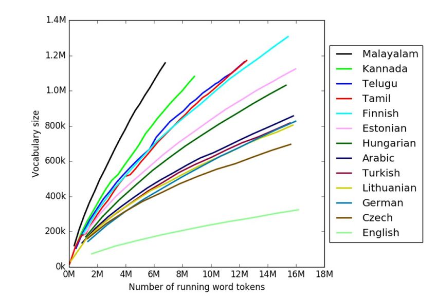
Reading material
●
Manning & Schütze, Foundations of Statistical Natural language
processing (1999) http://nlp.stanford.edu/fsnlp/
●
Jurafsky & Martin, Speechand Language Processing (3rd ed.
Draft, 2020) http://web.stanford.edu/~jurafsky/slp3/
●
Read the chapters corresponding to the lecture topics
Do not forget to study the
topic-specific reading material
(mentioned in slides) Statistical natural language processing 7/
7/
Lecture topics
1. 12 Jan Introduction & Project groups / Mikko Kurimo
2.    19 jan Statistical language models / Mikko Kurimo
3.    26 jan Word2vec / Tiina Lindh-Knuutila
4.    02 feb Sentence level processing / Mikko Kurimo
5.    09 feb Speech recognition / Janne Pylkkönen
6.    16 feb Chatbots and dialogue agents / Mikko Kurimo
7.    02 mar Statistical machine translation / Jaakko Väyrynen
8.    09 mar Morpheme-level processing / Mathias Creutz
9.    16 mar Neural language modeling and BERT / Mittul Singh
10.   23 mar Neural machine translation / Stig-Arne Grönroos
11.   30 mar Societal impacts and course conclusion / Krista Lagus, Mikko

                                                                            8/74
1. Introduction
What does language include?
What makes languages so complex?
What are the applications of statistical language
modeling?
9/74
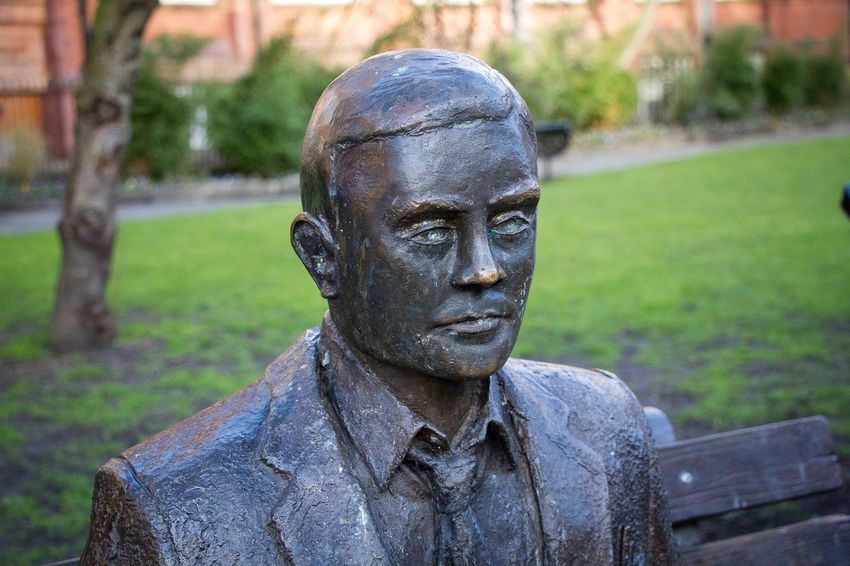
What is in a language?

 • Phonetics and phonology:
     • the physical sounds
     • the patterns of sounds
 • Morphology: The different building
   blocks of words
 • Syntax: The grammatical structure
 • Semantics: The meaning of words
 • Pragmatics, discourse, spoken
   interaction...
Complexity of languages
A large proportion of modern human activity
in its different forms is based on the use
of language
Large variation:
morphology and
syntactic structures
Complexity of natural language(s)
More than 6000 languages, many more dialects
Each language a large number of different word
forms
Each word is understood differently by each
speaker of a language at least to some degree 11/74Application areas
●
Information retrieval ●
Topic detection
●
Text clustering and ●
Sentiment analysis
classification ●
Word sense disambiguation
●
Automatic speech ●
Syntactic parsing
recognition
●
Text generation
●
Natural language
interfaces ●
Image, audio and video description
●
Statistical machine ●
Text-to-speech synthesis
translation ●
...
12/742. Statistical language modeling
N-gram LMs
Data sparsity problem
Equivalence classes
Back-off and interpolation
Smoothing methods, add-one, Good Turing,
Kneser-Ney
Maximum entropy LMs
Continuous space LMs
Neural network LMs
13/74Statistical Language Model
Model of a natural language that predicts the
probability distribution of words and sentences in a
text
Often used to determine which is the most probable
word or sentence in given conditions or context
Estimated by counting word frequencies and
dependencies in large text corpora
Has to deal with: big data, noisy data, sparse data,
computational efficiency
Statistical
Mikko Kurimo
natural language 14/
processingEstimation of N-gram model
c(“eggplant stew”)
c(“eggplant”)
Bigram example:
Start from a maximum likelihood estimate
probability
of P(“stew” | “eggplant”) is computed from counts of
“eggplant stew” and “eggplant”
works well for frequent bigrams
Why not for good rare bigrams?
Picture by B.Pellom
Statistical
Mikko Kurimo
natural language 15/
processingZero probability problem
If an N-gram is not seen in the corpus, it will get probability = 0
The higher N, the sparser data, and the more zero counts there will
be
20K words => 400M 2-grams => 8000G 3-grams, so even a
gigaword corpus has MANY zero counts!
Equivalence classes: Cluster several similar n-grams together to
reach higher counts
Smoothing: Redistribute some probability mass from seen N-grams
to unseen ones
Statistical
Mikko Kurimo
natural language 16/
processingSmoothing methods
1.Add-one: Add 1 to each count and normalize => gives too much probability to
unseen N-grams
2.(Absolute) discounting: Subtract a constant from all counts and redistribute this to
unseen ones using N-1 gram probs and back-off (normalization) weights
3.Witten-Bell smoothing: Use the count of things seen once to help to estimate the
count of unseen things
4.Good Turing smoothing: Estimate the rare n-grams based on counts of more
frequent counts
5.Best: Kneser-Ney smoothing: Instead of the number of occurrences, weigh the
back-offs by the number of contexts the word appears in
6.Instead of only back-off cases, interpolate all N-gram counts with N-1 counts
Statistical
Mikko Kurimo
natural language 17/
processingWeaknesses of N-grams
Skips long-span dependencies:
“The girl that I met in the train was ...”
Too dependent on word order:
“dog chased cat”: “koira jahtasi kissaa” ~ “kissaa koira jahtasi”
Dependencies directly between words, instead of latent variables,
e.g. word categories
Statistical
Mikko Kurimo
natural language 18/
processingMaximum entropy LMs
Represents dependency information
by a weighted sum of features f(x,h)
Features can be e.g. n-gram counts
Alleviates the data sparsity problem by smoothing the feature
weights (lambda) towards zero
The weights can be adapted in more flexible ways than n-grams
Adapting only those weights that significantly differ from a large
background model (1)
Normalization is computationally hard, but can be approximated
effectively
Mikko Kurimo
Speech recognition
2016 19/Continuous space LMs
Alleviates the data sparsity problem by representing words in a distributed
way
Various algorithms can be used to learn the most efficient and
discriminative representations and classifiers
The most popular family of algorithm is called (Artificial) Neural Networks
(NN)
can learn very complex functions by combining simple computation
units in a hierarchy of non-linear layers
Fast in action, but training takes a lot of time and labeled training data
Can be seen as a non-linear multilayer generalization of the maximum
entropy model
Mikko Kurimo
Speech recognition
2016 20/3. Vector space models for words and
documents
Vector space models, distributional semantics
word-document and word-word matrices
Constructing word vectors
stemming, weighting, dimensionality reduction
similarity measures
Count models vs. predictive models
Word2vec
Information retrieval
21/74Vector space models
Use a high-dimensional space for Applications:
documents and words – Document clustering and
• Closeness in the vector space classification
resembles closeness in the • Finding similar documents
semantics or structure of the • Finding similar words
documents (depending on the – Word disambiguation
features extracted). – Information retrieval
• Makes the use of data mining possible • Term discrimination: ranking
keywords by their usefulnessHow to build a vector space model? 1. Preprocessing 2. Defining word-document or word-word matrix • choosing features 3. Dimensionality reduction • choosing features • removing noise • easing computation 4. Weighting and normalization • emphasizing the features 5. Similarity / distance measures • comparing the vectors
To count or predict?

 Count-based methods                          Predictive models
 • compute the word co-occurrence             • try to predict a word from its neighbors
    statistics with its neighbor words in a      by directly learning a dense
    large text corpus                            representation
 • followed by a mapping (through
    weighting and dimensionality
    reduction) to dense vectors
Statistical semantics Statistical semantics hypothesis: Statistical patterns of human word usage can be used to figure out what people mean (Weaver, 1955; Furnas et al., 1983). Bag of words hypothesis: The frequencies of words in a document tend to indicate the relevance of the document to a query (Salton et al., 1975). Distributional hypothesis: Words that occur in similar contexts tend to have similar meanings (Harris, 1954; Firth, 1957; Deerwester et al., 1990). Latent relation hypothesis: Pairs of words that co-occur in similar patterns tend to have similar semantic relations (Turney et al., 2003).
Modifying the vector spaces

The basic matrix formulation offers lots of variations:
–window sizes
–word weighting, normalization, thresholding, removing stopwords
–stemming, lemmatizing, clustering, classification, sampling
–distance measures
–dimensionality reduction methods
–neural networks
Information retrieval: The query is compared to the
index and the best matching results are returned

                                         27/
Ranking the results Compute a numeric score on how well each object in the database matches the query – Distance in the vector space – Content and structure of the document collection – Number of hits in a document – Number of hits in title, first paragraph, elsewhere – Other meta information in the documents or external knowledge The retrieved objects are ranked according to the score and only the top ranking objects shown to the user.
4. Sentence-level processing
Tagging words in a sentence
Part-of-speech tagging
Named entity recognition
Solving ambiguities
Hidden Markov model, Viterbi, Baum-Welch,
Forward-Backward
Recurrent neural networks
Sentence parsing
Grammars, trees
Probabilistic context free grammar
29/74Part of Speech (POS) tagging
Task: Assign tags for each word in a sentence
Applications: Tool for parsing the sentence
The reaction in the newsroom was emotional.
=> DT NN IN DT NN VBD JJ
(determiner)
(noun) (preposition)
(determiner) (noun)
(verb past tense) (adjective)
Statistical
Mikko Kurimo
natural language 30/
processingNamed entity recognition
Detect names of persons, organizations, locations
Detect dates, addresses, phone numbers, etc
Applications: Information retrieval, ontologies
UN official Ekeus heads for Baghdad.
=> ORG - PER - - LOC
(organization) (person) (location)
Statistical
Mikko Kurimo
natural language 31/
processingA general approach
1.Generate candidates
2.Score the candidates
3.Select the highest scoring ones
Statistical
Mikko Kurimo
natural language 32/
processingA simple scoring method
Count the frequency of each tagging by listing all
appearances of the word in an annotated corpus
Select the most common tag for each word
How well would this method work?
Statistical
Mikko Kurimo
natural language 33/
processingCount transitions
Use the Penn Treebank corpus and count how often
each tag pair appears
Prepare a tag transition matrix
Compute transition probabilities from the counts
Just like bigrams for words, but now for tags
P(y1), P(y2|y1), P(y3|y2), P(y4|y3)
Statistical
Mikko Kurimo
natural language 34/
processingScore the tags for the sentence
Combine the transition probabilities:
P(y1) P(y2|y1) P(y3|y2) …
with the tag-word pair observation probabilites:
P(x1|y1) P(x2|y2) P(x3|y3)
to get the total tagging score:
P(y1)P(x1|y1) P(y2|y1)P(x2|y2) P(y3|y2)P(x3|y3)
Known as Hidden Markov Model (HMM) tagger
Achieves about 96% accuracy
Statistical
Mikko Kurimo
natural language 35/
processingHidden Markov model (HMM)
Markov chain assumes that the next state (tag)
depends only on the previous state (tag)
The states (tags) are hidden, we only see the words
The algorithm can compute the most likely state
sequence given the seen words
Statistical
Mikko Kurimo
natural language 36/
processingEstimation of HMM parameters
For corpora annotated with POS tags
Just count each tag observations P(y(t)|x(t)
And tag transitions P(y(t)|y(t-1))
For unknown data use e.g. Viterbi to first estimate
labels and then re-estimate parameters and iterate
Statistical
Mikko Kurimo
natural language 37/
processingEven better POS tags? Discriminative models
Use previous words and tags as features
The context is computed from a sliding window
Train a classifier to predict the next tag
Jurafsky: Maximum entropy Markov model (MEMM)
Support vector machine (SVM)
Deep (feed-forward) neural network (DNN)
Conditional random field (CRF) is a bidirectional extension
of MEMM that uses also tags on right
Statistical
Mikko Kurimo
natural language 38/
processingRecurrent neural network tagger
No fixed-length context window
Loop in the hidden layer adds an infinite memory
Can provide word-level tags:
POS or named entity
Or sentence-level tags:
Sentiment analysis
Topic or spam detection
Statistical
Mikko Kurimo
natural language 39/
processing5. Speech recognition
Acoustic features
Gaussian mixture models
Hidden Markov models
Deep neural networks for acoustic modeling
Phonemes, pronunciation of words
Decoding with language models
End-to-end neural networks
Encoder, Attention, Decoder
40/7441/74
42/74
Speech recognition: large probabilistic
              models

        Output: word sequence
                          Input: sound observations

    Decoding      Acoustic    Language
    algorithm      model        model

                                                      43/74
6. Chatbots and dialogue agents
True chatbots vs task-oriented dialogue agents
Text processing steps in chatbots
Chatbot architectures
Evaluation of chatbots
44/74Definitions Chatbot: • A system that you can chat with • Discussion topics can be fixed, but there is no specific goal except for fun and keeping company Dialogue agent: • A system that helps you to reach a specific goal by giving and collecting information by answering and asking questions In popular media both are often called chatbots, but here only the first one.
Comparison of chatbots and dialogue
agents: required operations
Chatbot
Detect the discussion topic
Ask typical questions
React to human input, be coherent
with previous turns
World knowledge, persona
Dialogue agent
Detect the user's intent
Ask the required questions
Parse and use human inputChatbot architectures
Rule-based
• Pattern-action rules: Eliza (1966)
• Mental model: Parry (1971)
Corpus-based
• IR: Cleverbot
• DNN encoder-decoders etc
Turing’s test (1950) for machine
intelligence: Can you judge between a
real human and a chatbot?Evaluation of chatbots
Automatic evaluation Human evaluation
Lack of proper evaluation data and metrics e.g. research challenges
N-gram matching evaluations such as BLEU (competitions):
correlate poorly with human evaluation
ConvAI (NeurIPS)
Too many correct answers
Dialog Systems
Common words give a good score Technology Challenge
Perplexity measures predictability using a language (DSTC7)
model
Amazon Alexa prize
Favours short, boring and repetitive answers
Loebner Prize
ADEM classifier trained by human judgements
Adversarial evaluation trained to distinguish human
and machine responses7. Statistical machine translation
Sentence, word and phrase alignment methods
Re-ordering models
Translation methods
Full SMT systems
49/74Machine translation:
large probabilistic models
50/74Phrase-based SMT system
Training data and data preprocessing
Word aligment, phrase aligment
Estimation of translation model scores
Estimation of reordering model scores
Estimation of language model scores
Decoding algorithm and optimization of the model
weights
Translation, recasing, detokenization
Evaluation, quality estimation
Operational management
51/74Sentence Alignment
Simplifying assumptions: monotonic, break on
paragraphs
Gale&Church algorithm: model sentence lengths
Other features: (automatic) dictionaries, cognates
Dynamic programming (Similar to Viterbi)
52/74Word Alignment
The sentence alignment was the first step
The word alignment takes into account
reordering (distortion)
fertility of the words
Iterative Expectation-Maximization algorithm:
1. Generate a word level alignment using estimated
translation probabilities
2. Estimate translation probabilities for word pairs
from the alignment
53/74Phrase alignment
“Cut-and-paste" translation
The distortion (reordering) probability typically
penalizes more, if several words have to be reordered.
However, usually larger multi-word chunks
(subphrases) need to be moved
Algorithms to learn a phrase translation table
Re-ordering models
54/74Translation methods
Phrase-based beam-search decoder (e.g. Moses)
Weighted finite state transducer (WFST) based
translation models
Extended word-level representations, e.g., hierarchical
phrase-based models and factored translation models
with words augmented with POS tags, lemmas, etc.
Syntax-based translation models, which take syntax
parse trees as input.
Feature-based models, where translation is performed
between features. E.g., discriminative training or
exponential models over feature vectors
55/748. Morpheme-level processing
Morphemes
morphological complexity, processes, models
Morphological clustering
stemming, lemmatization
Morphological analysis and generation
Finite-state methods, transducers
Morphological segmentation
Zellig Harris's method
Morfessor
56/74Types of morphemes
• Root: a portion of word without any affixes; carries the principle portion of
meaning (buildings build)
• Stem: a root, or compound of roots together with derivational affixes
(buildings building)
• Affix: a bound morpheme (does not occur by itself) that is attached before,
after, or inside a root or stem
• Prefix (un-happy)
• Suffix (build-ing, happi-er)
• Infix (abso-bloody-lutely)
• …
06/03/
57 –
Statistical Natural Language Processing 19
Morpheme-level processingMorphology affects the vocabulary size
Vocabulary size as a
function of corpus size
Varjokallio, Kurimo, Virpioja (2016)
06/03/
58 –
Statistical Natural Language Processing 19
Morpheme-level processingMorphological processes
Inflection:
• cat – cats
• slow – slower
• find – found
Derivation:
• build (V) – building (N)
• do (V) – doable (ADJ)
• short (ADJ) – shorten (V)
• write – rewrite
• do – undo
Compounding:
• fireman (fire + man)
• hardware (hard + ware)
06/03/
59 –
Statistical Natural Language Processing 19
Morpheme-level processing3 main approaches to deal with rich morphology
1. “Canonical” forms of a word
• Stemming is relatively simple and implementations are available, for
English: e.g., Porter (1980), Snowball: http://snowball.tartarus.org
• Lemmatization is more complex and needs morphological analysis
• Applications: Information retrieval etc.
2. Morphological analysis
• Hand-crafted morphological analyzers/generators exist for many
languages, e.g. Tähtien => tähti N Gen Pl
• Applications: Spell checking, syntactic parsers, machine translation, etc.
3. Segmentation into morphs
• Pragmatic approaches that work well enough in practice.
• Applications: Speech recognition, language modeling etc.
06/03/
60 –
Statistical Natural Language Processing 19
Morpheme-level processingLimitations of morphological analysis
Out-of-vocabulary words
• epäjärjestelmällistyttämättömyydelläänsäkäänköhän
epäjärjestelmällistyttämättömyydelläänsäkäänköhän+?
Ambiguous forms
• sawsee+V+PAST or saw+N or saw+V+INF ?
“I saw her yesterday.” SEE (verb)
“The saw was blunt.” SAW (noun)
“Don’t saw off the branch you are sitting on.” SAW (verb)
• meetingmeet+V+PROG or meeting+N ?
“We are meeting tomorrow.” MEET (verb)
“In our meeting, we decided not to meet again.” MEETING (noun)
• Solutions?
06/03/
61 –
Statistical Natural Language Processing 19
Morpheme-level processingUnupervised morphological segmentation
… …
• Morphological segmentation aamu aamu
• Send a vocabulary of the language aamua aamu a
aamuaurinko aamu aurinko
over a channel with limited band-
aamukahvi aamu kahvi
width. aamuksi aamu ksi
• compress the vocabulary. aamulehti aamu lehti
• What regularities can we exploit? aamulla aamu lla
aamun aamu n
• Use morphemes, the smallest aamunaamasi aamu naama si
?
meaning-bearing units of aamupalalla aamu pala lla
language? aamupalan aamu pala n
aamupostia aamu posti a
• Morfessor method (Creutz & aamupäivä aamu päivä
Lagus, 2002) aamupäivällä aamu päivä llä
aamuyö aamu yö
aamuyöllä aamu yö llä
aamuyöstä aamu yö stä
… …
06/03/
62 –
Statistical Natural Language Processing 19
Morpheme-level processingMorfessor
• Instead of sending over the vocabulary as it is, we split it into two parts:
1. a fairly compact lexicon of morphs: “aamu”, “aurinko”, “ksi”, “lla”, …
2. the word vocabulary expressed as sequences of morphs
• Since we are doing unsupervised learning, we do not know the correct
answer.
• Our target is to minimize the combined code length of:
1. the code length of the morph lexicon
2. plus the code length of the word vocabulary expressed using the
morph lexicon.
06/03/
63 –
Statistical Natural Language Processing 19
Morpheme-level processingImproved Morfessor model
Software: http://morpho.aalto.fi
• A later context-sensitive version of Morfessor introduces three categories: stem (STM), prefix (PRE) and suffix
(SUF) that each morph must belong to.
• A word form must have the structure of the following regular expression: ( PRE* STM SUF* )+
• From the updated examples below, you can see that many issues have been fixed, but the model is still fairly
crude; for instance, it suggests two consecutive s-suffixes in the word “abyss”: aby s s.
abandon/STM ed/SUF absolute/STM differ/STM present/STM ed/SUF
abandon/STM ing/SUF absolute/STM ly/SUF differ/STM ence/STM present/STM ing/SUF
abb/STM absorb/STM differ/STM ence/STM s/SUF present/STM ly/SUF
abby/STM absorb/STM ing/SUF different/STM present/STM s/SUF
abdel/STM absurd/STM differential/STM preserv/STM e/SUF
able/STM absurd/STM ity/SUF different/STM ly/SUF preserv/STM e/SUF s/SUF
ab/STM normal/STM abt/STM differ/STM ing/SUF provide/STM s/SUF
aboard/STM abu/STM difficult/STM provi/STM ding/STM
about/STM abuse/STM difficult/STM i/SUF es/SUF pull/STM ed/SUF
abroad/STM abuse/STM d/SUF difficult/STM y/SUF pull/STM er/SUF s/SUF
abrupt/STM ly/SUF ab/STM users/STM dig/STM pull/STM ing/SUF
absence/STM abuse/STM s/SUF digest/STM pump/STM
absent/STM aby/STM s/SUF s/SUF digital/STM pump/STM ed/SUF
absent/STM ing/SUF accent/STM diglipur/STM pump/STM ing/SUF
06/03/ 64
Statistical Natural Language Processing – 19
Morpheme-level processing9. Neural Network LM
Feed-Forward and Recurrent NNLM
NNLM training
Various architectures and modeling units
Model combination
65/74A linear bigram NN LM
Outputs the probability of next word y(t) given the previous word x(t)
Input layer maps the previous word as a vector x(t)
Hidden layer has a linear transform h(t) = Ax(t) + b to compute a
representation of linear distributional features
Output layer maps the values by y(t) = softmax (h(t)) to range (0,1) that
add up to 1
Resembles a bigram Maximum entropy LM
Softmax: Ax+b softmax
h(t)
x(t) y(t)
Mikko Kurimo
Speech recognition
2016 66/A non-linear bigram NN LM
The hidden layer h(t) includes a non-linear function h(t) = U(Ax(t) + b)
Can learn more complex feature representations
Common examples of non-linear functions U:
U (t) = tanh (t)
Sigmoid U V
h(t)
U
x(t) y(t)
Mikko Kurimo 2016 Speech recognition 67/Common NN LM extensions
Input layer is expanded over
several previous words x(t-1), x(t-
2), .. to learn richer
representations
c(t)
Deep neural networks have
several hidden layers h1, h2, .. to
learn to represent information at
several hierarchical levels
Can be scaled to a very large U1 U2 V
vocabulary by training also a
class-based output layer c(t) h1(t) h2(t)
x(t-2)
y(t)
x(t-1)
x(t)
Mikko Kurimo 2016 Speech recognition 68/Recurrent Neural Network (RNN) LM
Looks like a bigram NNLM h(t-1)
But, takes an additional input from the
hidden layer of the previous time step
Hidden layer becomes a compressed
representation of the word history W
Can learn to represent unlimited
memory, in theory
U V
Currently, the state-of-the-art in LMs
h(t)
x(t) y(t)
Mikko Kurimo 2016 Speech recognition 69/10. Neural machine translation
Neural machine translation
Why NMT is the mainstream ∗ approach? approach?
How are the current NMT systems build?
What are the challenges and limitations for the systems?
Evaluation of machine translation
How machine translation systems are evaluated manually?
How do the standard automatic metrics work and how they can
be improved?
What are the limitations of the metrics?
70/74Why NMT?
Generalization
Flexibility
Integration
71/74Building NMT
Encoding variable-length sequences
Sequence decoding
Sequence-to-sequence models
Recurrent neural networks
Attention model, Transformer model
Modeling units
72/74Evaluation of machine translation
Human evaluation
Assessment, ranking, agreement, efficiency
Automatic evaluation
Challenges?
Edit distance metrics
Precision & recall, BLEU
Beyond word-based metrics
Meta-evaluation
Evaluation of evaluation metrics
73/74Lecture topics
1. 12 Jan Introduction & Project groups / Mikko Kurimo
2. 19 jan Statistical language models / Mikko Kurimo
3. 26 jan Word2vec / Tiina Lindh-Knuutila
4. 02 feb Sentence level processing / Mikko Kurimo
5. 09 feb Speech recognition / Janne Pylkkönen
6. 16 feb Chatbots and dialogue agents / Mikko Kurimo
7. 02 mar Statistical machine translation / Jaakko Väyrynen
8. 09 mar Morpheme-level processing / Mathias Creutz
9. 16 mar Neural language modeling and BERT / Mittul Singh
10. 23 mar Neural machine translation / Stig-Arne Grönroos
11. 30 mar Societal impacts and course conclusion / Krista Lagus, Mikko
74/74You can also read