Segmenting two-dimensional structures with strided tensor networks
←
→
Page content transcription
If your browser does not render page correctly, please read the page content below
Segmenting two-dimensional structures with
                                                       strided tensor networks

                                                     Raghavendra Selvan1,2 , Erik B Dam1 , and Jens Petersen1,3
                                                     1
                                                         Department of Computer Science, University of Copenhagen
                                                         2
                                                           Department of Neuroscience, University of Copenhagen
arXiv:2102.06900v1 [cs.CV] 13 Feb 2021

                                                           3
                                                             Department of Oncology, Rigshospitalet, Denmark
                                                                           raghav@di.ku.dk

                                                 Abstract. Tensor networks provide an efficient approximation of opera-
                                                 tions involving high dimensional tensors and have been extensively used
                                                 in modelling quantum many-body systems. More recently, supervised
                                                 learning has been attempted with tensor networks, primarily focused on
                                                 tasks such as image classification. In this work, we propose a novel formu-
                                                 lation of tensor networks for supervised image segmentation which allows
                                                 them to operate on high resolution medical images. We use the matrix
                                                 product state (MPS) tensor network on non-overlapping patches of a
                                                 given input image to predict the segmentation mask by learning a pixel-
                                                 wise linear classification rule in a high dimensional space. The proposed
                                                 model is end-to-end trainable using backpropagation. It is implemented
                                                 as a strided tensor network to reduce the parameter complexity. The
                                                 performance of the proposed method is evaluated on two public medi-
                                                 cal imaging datasets and compared to relevant baselines. The evaluation
                                                 shows that the strided tensor network yields competitive performance
                                                 compared to CNN-based models while using fewer resources. Addition-
                                                 ally, based on the experiments we discuss the feasibility of using fully
                                                 linear models for segmentation tasks. 4
                                                 Keywords: tensor networks · linear models · image segmentation

                                         1     Introduction
                                         Large strides made in the quality of computer vision in the last decade can be
                                         attributed to deep learning based methods [10]; in particular, to the auxiliary
                                         developments (powerful hardware, better optimisers, tricks such as dropout, skip
                                         connections etc.) that have made convolutional neural networks (CNNs) more
                                         effective. This has also influenced biomedical image segmentation with models
                                         such as the U-net [22] which have become widely popular5 .
                                             Tensor networks are factorisations of high dimensional tensors, and have been
                                         widely used to study quantum many-body systems [16]. Conceptually, they can
                                         be interpreted as linear models operating in high dimensional spaces, in con-
                                         trast to neural networks which are highly non-linear models operating in lower
                                         dimensional spaces. Tensor networks have been used as feature extractors [2],
                                         4
                                             Source code: https://github.com/raghavian/strided-tenet
                                         5
                                             First author of [22] noted their U-net work was cited more than once every hour in
                                             2020. https://bit.ly/unet2020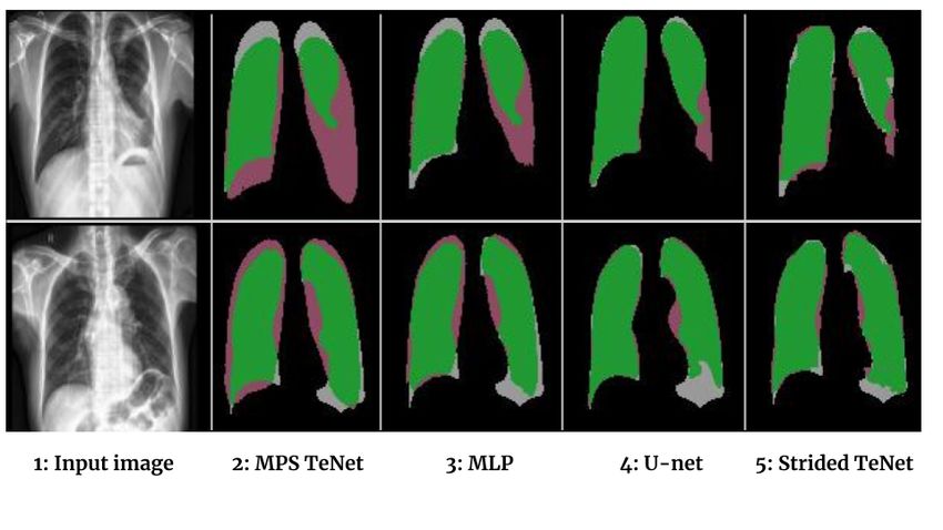
2        R. Selvan et al.

predictors operating in very high dimensional spaces [13] and to compress neural
networks [15]. More recently, they are also being studied in the context of su-
pervised learning with growing success [25,5,23]. They have been primarily used
for image classification [25,5] and most recently to classify medical images [23].
Tensor networks have not been studied for image segmentation to the best of
the authors’ knowledge.
    In this work, we propose the strided tensor network: a tensor network based
image segmentation method. Tensor network operations are performed on image
patches to learn a hyper-plane that classifies pixels into foreground and back-
ground classes in a high dimensional space. This is similar to classical pixel
classification methods operating in some expressive feature space [24,26]. The
key difference with tensor networks is that they do not require designed features
that encode domain specific knowledge, and still are able to learn linear mod-
els that are competitive with state-of-the-art CNN-based models, as has been
shown for tasks such as image classification [5,23]. Further, the proposed model
can be trained in an end-to-end manner in a supervised learning set-up by back-
propagating a relevant loss function. We experiment on two biomedical imaging
datasets: to segment nuclei from microscopy images of multi-organ tissues, and
to segment lungs from chest X-rays (CXR). We compare the strided tensor net-
work with relevant baselines, including deep learning models, and demonstrate
that the tensor network based model can yield similar performance compared to
CNN-based models with fewer resources.

2     Methods
2.1     Overview

In this work, we propose a tensor network based model to perform image seg-
mentation. This is performed by approximating the segmentation decision as a
linear model in an exponentially high dimensional space. That is, we are inter-
ested in deriving a hyper-plane in a high dimensional space such that it is able
to classify pixels into foreground and background classes across all images in the
dataset.
    We consider non-overlapping image patches, flatten them into 1D vectors
and apply simple sinusoidal feature transformations resulting in local feature
maps. By taking tensor product of these local feature maps, we obtain global
feature maps which in effect lift the input image patch into an exponentially
high dimensional space. Weights for the linear model that operate on the global
feature maps, resulting in segmentation predictions, are approximated using the
matrix product state (MPS) tensor network6 [19,17]. The same trainable MPS
is used on non-overlapping image patches from the entire image resulting in our
strided tensor network model for image segmentation. Predicted segmentations
are compared with ground truth labels in the training set to obtain a suitable
loss which is backpropagated to optimise the weights of our model. A high level
overview of the proposed model is illustrated in Figure 1.
6
    Matrix product state is also known as Tensor Trains in literature.
Strided Tensor Networks        3

Fig. 1. a) High level overview of the proposed strided tensor network model. Matrix
product state (MPS) operations are performed on non-overlapping regions of the input
image, X, of size H×W resulting in the predicted segmentation, S. Loss computed
between prediction, S, and the ground truth, Y , are backpropagated during training.
Arrows on MPS block are used to indicate that the same MPS block is applied across
the image. b) In practice, the strided tensor network operations can be accelerated
using batch processing by creating non-overlapping patches (size K×K) on the fly
as input to MPS, and tiling these batched predictions to reconstruct the full image
segmentation.

    In the remainder of this section, we present a brief introduction to tensor
notation, describe the choice of local feature maps, going from local to global
feature maps and details on approximating the segmentation rule with MPS, in
order to fully describe the proposed strided tensor network for image segmenta-
tion.

2.2   Tensor notation

Tensor notations are concise graphical representations of high dimensional ten-
sors introduced in [18]. A grammar of tensor notations has evolved through the
years enabling representation of complex tensor algebra. This not only makes
working with high dimensional tensors easier but also provides insight into how
they can be efficiently manipulated. Figure 2 shows the basics of tensor nota-
tions and one important operation – tensor contraction (in sub-figures b & c).
We build upon the ideas of tensor contractions to understand tensor networks
such as the MPS, which is used extensively in this work. For more detailed
introduction to tensor notations we refer to [3].

2.3   Image segmentation using linear models

In order to motivate the need for using patches, we first describe the model at
the full image level.
    Consider a 2 dimensional image, X ∈ RH×W ×C with N = H × W pixels and
C channels. The task of obtaining an M –class segmentation, Y ∈ {0, 1}H×W ×M
is to learn the decision rule of the form f (· ; Θ) : X 7→ Y , which is parameterised
by Θ. These decision rules, f (· ; Θ), could be non-linear transfer functions such
as neural networks. In this work, building on the success of tensor networks used
for supervised learning [25,5,23], we explore the possibility of learning f (· ; Θ)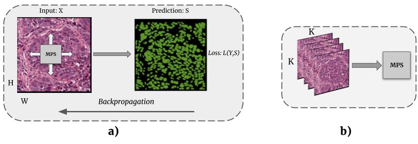
4        R. Selvan et al.

Fig. 2. a) Graphical tensor notation depicting an order-0 tensor (scalar S), order-1
tensor (vector V i ), order-2 tensor (matrix M ij ) and an order-3 tensor T ijk . Tensor
indices – seen as the dangling edges – are written as superscripts by convention. b)
Illustration of < M, P >: the dot product of two order-3 tensors of dimensions i = 4, j =
3, k = 2. c) Tensor notation depicting the same dot product between the tensors Mijk
and Pijk . Indices that are summed over (tensor contraction) are written as subscripts.
Tensor notations can capture operations involving higher order tensors succinctly.

that are linear. For simplicity, we assume two class segmentation of single channel
images, implying M = 1, C = 1. However, extending this work to multi-class
segmentation of inputs with multiple channels is straightforward.
     Before applying the linear decision rule, the input data is first lifted to an ex-
ponentially high dimensional space. This is based on the insight that non-linearly
separable data in low dimensions could possibly become linearly separable when
lifted to a sufficiently high dimensional space [4]. The lift in this work is accom-
plished in two steps.
     First, the image is flattened into a 1-dimensional vector x ∈ RN . Simple
transformations are applied to each pixel to increase the number of features per
pixel. These increased features are termed local feature maps. Pixel intensity-
based local feature maps have been explored in recent machine learning applica-
tions of tensor networks [5,21,23]. We use a general sinusoidal local feature map
from [25], which increases local features of a pixel from 1 to d:
               s
                    d−1          π     (d−ij )      π    (ij −1)
      ij
    ψ (xj ) =                 cos( xj )            sin( xj )         ∀ ij = 1 . . . d. (1)
                    ij − 1        2                    2

The intensity values of individual pixels, xj , are assumed to be normalised to be
in [0, 1]. Further, the local feature maps are constrained to have unit norm so
that the global feature map in the next step also has unit norm.
    In the second step, a global feature map is obtained by taking the tensor
product7 of the local feature maps. This operation takes N order-1 tensors and
                                                  N
outputs an order-N tensor, Φi1 ...iN (x) ∈ [0, 1]d given by

                  Φi1 ...iN (x) = ψ i1 (x1 ) ⊗ ψ i2 (x2 ) ⊗ · · · ⊗ ψ iN (xN ).       (2)

Note that after this operation each image can be treated as a vector in the dN
dimensional Hilbert space [16,25].
7
    Tensor product is the generalisation of matrix outer product to higher order tensors.
Strided Tensor Networks 5
Given the dN global feature map in Equation (2), a linear decision function
f (·; Θ) can be estimated by simply taking the tensor dot product of the global
feature map with an order-(N+1) weight tensor, Θim1 ...iN :
f m (x ; Θ) = Θim1 ...iN · Φi1 ...iN (x). (3)
The additional superscript index m on the weight tensor and the prediction
is the output index of dimension N . That is, the resulting order-1 tensor from
Equation (3) has N entries corresponding to the pixel level segmentations. Equa-
tion (3) is depicted in tensor notation in Figure 3-a.
2.4 Strided tensor networks
While the dot product in Equation (3) looks easy enough conceptually, on closer
inspection its intractability comes to light. The approach used to overcome this
intractability leads us to the proposed strided tensor network model.
1. Intractability of the dot product: The sheer scale of the number of
parameters in the weight tensor Θ in Equation (3) can be mind boggling.
For instance, the weight tensor required to operate on an tiny input image
of size 16×16 with local feature map d = 2 is N · dN = 1024 · 21024 ≈ 1079
which is close to the number of atoms in the observable universe8 (estimated
to be about 1080 ).
2. Loss of spatial correlation: The assumption in Equations (1), (2) and (3)
is that the input is a 1D vector. Meaning, the 2D image is flattened into a 1D
vector. For tasks like image segmentation, spatial structure of the images can
be informative in making improved segmentation decisions. Loss of spatial
pixel correlation can be detrimental to downstream tasks; more so when
dealing with complex structures encountered in medical images.
We overcome these two constraints by approximating the linear model in Equa-
tion (3) using MPS tensor network and by operating on strides of smaller non-
overlapping image patches.
Matrix Product State Computing the inner product in Eq. (3) becomes in-
feasible with increasing N [25]. It also turns out that only a small number of
degrees of freedom in these exponentially high dimensional Hilbert spaces are
relevant [20,16]. These relevant degrees of freedom can be efficiently accessed
using tensor networks such as the MPS [19,17]. In image analysis, accessing this
smaller sub-space of the high dimensional Hilbert space corresponds to accessing
interactions between pixels that are local either in spatial- or in some feature-
space sense that is relevant for the task.
MPS is a tensor factorisation method that can approximate any order-N
tensor with a chain of order-3 tensors. This is visualized using tensor notation
i
in Figure 3-b for approximating Θim1 ...iN using Aαjj αj+1 ∀ j = 1 . . . N which are
of order-3 (except on the borders where they are order-2). The dimension of
8
https://en.wikipedia.org/wiki/Observable_universe6 R. Selvan et al.
subscript indices of αj which are contracted can be varied to yield better ap-
proximations. These variable dimensions of the intermediate tensors in MPS are
known as bond dimension β. MPS approximation of Θim1 ...iN depicted in Fig-
ure 3-b is given by
X
Θim1 ...iN = Aiα11 Aiα21 α2 Aiα32 α3 . . . Am,i iN
αj αj+1 . . . AαN .
j
(4)
α1 ,α2 ,...αN
i
The components of these intermediate lower-order tensors Aαjj αj+1 ∀ j = 1 . . . N
form the tunable parameters of the MPS tensor network. This MPS factorisation
in Equation (4) reduces the number of parameters to represent Θ from N · dN
to {N · d · N · β 2 } with β controlling the quality of these approximations9 . Note
that when β = dN/2 the MPS approximation is exact [16,25].
Various implementations of MPS per-
form the sequence of tensor contrac-
tions in different ways for efficiency.
We use the TorchMPS implementa-
tion in this work, which first con-
tracts the horizontal edges and performs
tensor contractions along the vertical
edges [12,23].
MPS on non-overlapping patches
The issue of loss in spatial pixel correla-
tion is not alleviated with MPS as it oper-
ates on flattened input images. MPS with Fig. 3. a) Linear decision rule in
higher bond dimensions could possibly al- Equation 3 depicted in tensor nota-
low interactions between all pixels but, tion. Note that Θ has N+1 edges as
due to the quadratic increase in number it is an order-(N+1) tensor. The d-
of parameters with the bond dimension β, dimensional local feature maps are the
i
working with higher bond dimensions can gray nodes marked ψ j (xj ). b) Ma-
be prohibitive. trix product state (MPS) approxima-
To address this issue, we apply MPS tion of Θ in Equation 4 into a tensor
train comprising up to order-3 tensors,
on small non-overlapping image regions. i
Aαjj αj+1 .
These smaller patches can be flattened
without severe degradation of spatial cor-
relation. Similar strategy of using MPS on small image regions has been used
for image classification using tensor networks in [23]. This is also in the same
spirit of using convolutional filter kernels in CNNs when the kernel width is set
to be equal to the stride length. This formulation of using MPS on regions of
size K × K with a stride equal to K in both dimensions results in the strided
tensor network formulation, given as
f (x; ΘK ) = {ΘK · Φ(x(i,j) )} ∀ i = 1, . . . , H/K, j = 1, . . . , W/K (5)
9
Tensor indices are dropped for brevity in the remainder of the manuscript.Strided Tensor Networks 7
Fig. 4. (First four columns) Sample images from the MO-Nuseg dataset comprising
histopathology slides from multiple organs (top row) and the corresponding binary
masks (bottom row). (Last four columns) Sample chest X-ray images from the Lung-
CXR dataset with corresponding binary masks.
where (i, j) are used to index the patch from row i and column j of the image
grid with patches of size K × K. The weight matrix in Equation (5), ΘK is
subscripted with K to indicate that MPS operations are performed on K × K
patches.
In summary, with the proposed strided tensor network formulation, linear
segmentation decisions in Equation (3) are approximated at the patch level using
MPS. The resulting patch level predictions are tiled back to obtain the H × W
segmentation mask.
2.5 Optimisation
The weight tensor, ΘK , in Equation (5) and in turn the lower order tensors in
Equation (4) which are the model parameters can be learned in a supervised set-
ting. For a given labelled training set with T data points, D : {(x1 , y1 ), . . . (xT , yT )},
the training loss to be minimised is
T
1X
Ltr = L(f (xi ), yi ), (6)
T t=1
where yi are the binary ground truth masks and L(·) can be a suitable loss
function suitable for segmentation tasks. In this work, as both datasets were
largely balanced (between foreground and background classes) we use binary
cross entropy loss.
3 Data & Experiments
Segmentation performance of the proposed strided tensor network is evaluated
on two datasets and compared with relevant baseline methods. Description of
the data and the experiments are presented in this section.
3.1 Data
MO-NuSeg Dataset The first dataset we use in our experiments is the multi-
organ nuclei segmentation (MO-NuSeg) challenge dataset10 [8]. This dataset con-
sists 44 Hematoxylin and eosin (H&E) stained tissue images, of size 1000×1000,
10
https://monuseg.grand-challenge.org/8 R. Selvan et al.
with about 29,000 manually annotated nuclear boundaries. The dataset has tis-
sues from seven different organs and is a challenging one due to the variations
across different organs. The challenge organizers provide a split of 30 train-
ing/validation images and 14 testing images which we also follow to allow for
comparisons with other reported methods. Four training tissue images and the
corresponding binary nuclei masks are shown in the first four columns of Fig-
ure 4.
Lung-CXR Dataset We also use the lung chest X-ray dataset collected from
the Shenzhen and Montgomery hospitals with posterio-anterior views for tuber-
culosis diagnosis [7]. The CXR images used in this work are of size 128×128
with corresponding binary lung masks for a total of 704 cases which is split into
training (352), validation (176) and test (176) sets. Four sample CXRs and the
corresponding binary lung masks are shown in the last four columns of Figure 4.
3.2 Experiments
Experimental set-up The proposed strided tensor network model was com-
pared with a convolutional neural network (U-net [22]), a modified tensor net-
work (MPS TeNet) that uses one large MPS operation similar to the binary
classification model in [5], and a multi-layered perceptron (MLP). Batch size of
1 and 32 were used for the MO-NuSeg and Lung-CXR datasets, respectively,
which was the maximum batch size usable with the baseline U-net; all other
models were trained with the same batch size for a fairer comparison. The mod-
els were trained with the Adam optimizer and an initial learning rate of 5×10⁻⁴ ,
except for the MPS TeNet which required smaller learning rate of 1 × 10⁻⁵ for
convergence; they were trained until there was no improvement in validation
accuracy for 10 consecutive epochs. The model based on the best validation
performance was used to predict on the test set. All models were implemented
in PyTorch and trained on a single GTX 1080 graphics processing unit (GPU)
with 8GB memory. The development and training of all models in this work was
estimated to produce 61.9 kg of CO2eq, equivalent to 514.6 km travelled by car
as measured by Carbontracker11 [1].
Metrics Performance of the different methods for both datasets are compared
using Dice score based on binary predictions, ŷi ∈ {0, 1} obtained by thresh-
olding soft segmentations at 0.5 which we recognise is an arbitrary threshold. A
more balanced comparison is provided using the area under the precision-recall
curve (PRAUC or equivalently the average precision) using the soft segmenta-
tion predictions, si ∈ [0, 1].
Model hyperparameters The initial number of filters for the U-net model was
tuned from [8, 16, 32, 64] and a reasonable choice based on validation performance
and training time was found to be 8 for MO-NuSeg dataset and 16 for Lung-
CXR dataset. The MLP consists of 6 levels, 64 hidden units per layer and ReLU
activation functions and was designed to match the strided tensor network in
11
https://github.com/lfwa/carbontracker/Strided Tensor Networks 9
Table 1. Test set performance comparison for segmenting nuclei from the stained
tissue images (MO-NuSeg) and segmenting lungs from chest CT (Lung-CXR). For all
models, we report the number of parameters |Θ|, computation time per training epoch,
area under the curve of the precision-recall curve (PRAUC) and average Dice accuracy
(with standard deviation over the test set). The representation (Repr.) used by each
of the methods at input is also mentioned.
Dataset Models Repr. |Θ| t(s) PRAUC Dice
Strided TeNet (ours) 1D 5.1K 21.2 0.78 0.70 ± 0.10
U-net [22] 2D 500K 24.5 0.81 0.70 ± 0.08
MO-NuSeg
MPS TeNet [5] 1D 58.9M 240.1 0.55 0.52 ± 0.09
CNN 2D – 510 – 0.69 ± 0.10
Strided TeNet (ours) 1D 2.0M 6.1 0.97 0.93 ± 0.06
U-net [22] 2D 4.2M 4.5 0.98 0.95 ± 0.02
Lung-CXR
MPS TeNet [5] 1D 8.2M 35.7 0.67 0.57 ± 0.09
MLP 1D 2.1M 4.1 0.95 0.89 ± 0.05
number of parameters. The strided tensor network has two critical hyperparam-
eters: the bond dimension (β) and the stride length (K), which were tuned using
the validation set performance. The bond dimension controls the quality of the
MPS approximations and was tuned from the range β = [2, 4, 8, 12, 16, 20, 24].
The stride length controls the field of view of the MPS and was tuned from the
range K = [2, 4, 8, 16, 32, 64, 128]. For MO-NuSeg dataset, the best validation
performance was stable for any β ≥ 4, so we used the smallest with β = 4 and
the best performing stride parameter was K = 8. For the Lung-CXR dataset
similar performance was observed with β ≥ 20, so we set β = 20 and obtained
K = 32. The local feature dimension (d) was set to 4 (see Section 4 for additional
discussion on local feature maps).
3.3 Results
MO-NuSeg Performance of the strided tensor network compared to the baseline
methods on the MO-NuSeg dataset are presented in Table 1 where we report
the PRAUC, Dice accuracy, number of parameters and the average training time
per epoch for all the methods. Based on both PRAUC and Dice accuracy, we
see that the proposed strided tensor network (PRAUC=0.78, Dice=0.70) and
the U-net (PRAUC=0.81, Dice=0.70) obtain similar performance. There was no
significant difference between the two methods based on paired sample t-tests.
The Dice accuracy reported in the paper that introduced the dataset12 in [8]
(0.69) is also in the same range as the reported numbers for the strided tensor
network. A clear performance difference is seen in comparison to the MPS tensor
network (PRAUC=0.55, Dice=0.52); the low metrics for this method is expected
as it is primarily a classification model [5] modified to perform segmentation to
12
These numbers are reported from [8] for their CNN2 model used for binary seg-
mentation. Run time in Table 1 for CNN2 model could be lower with more recent
hardware.10 R. Selvan et al.
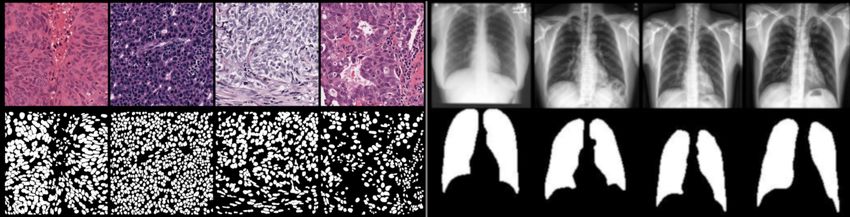
Fig. 5. Two test set CXRs from Lung-CXR dataset along with the predicted segmen-
tations from the different models. All images are upsampled for better visualisation.
(Prediction Legend – Green: True Positive, Grey: False Negative, Pink: False Positive)
compare with the most relevant tensor network.
Lung-CXR dataset Segmentation accuracy of the strided tensor network is
compared to U-net, MPS tensor network and MLP on the Lung-CXR dataset in
Table 1. U-net (0.98) and the proposed strided tensor network (0.97) attain very
high PRAUC, and the Dice accuracy for strided tensor network is 0.93 and for
U-net it is 0.95; there was no significant difference based on paired sample t-test.
Two test set predictions where the strided tensor network had high false positive
(top row) and high false negative (bottom row), along with the predictions from
other methods and the input CXR are shown in Figure 5.
4 Discussion & Conclusions
Results from Table 1 show that the proposed strided tensor network compares
favourably to other baseline models across both datasets. In particular, to the
U-net where there is no significant difference in Dice accuracy and PRAUC. The
computation cost per training epoch of strided tensor network is also reported in
Table 1. The training time per epoch for both datasets for the proposed strided
tensor network is in the same range of those for U-net. In multiple runs of
experiments we noticed that U-net converged faster (≈ 50 epochs) whereas the
tensor network model converged around 80 epochs. Overall, the training time for
tensor network models on both datasets was under one hour. A point also to be
noted is that operations for CNNs are highly optimised in frameworks such as
PyTorch. More efficient implementations of tensor network operations are being
addressed in recent works [6,14] and the computation cost is expected to reduce
further.
An additional observation in the experiments on MO-NuSeg data, reported
in Table 1 is the number of parameters used by the strided tensor network (5.1K)
which is about two orders of magnitude smaller than that of the U-net (500K),
without a substantial difference in segmentation accuracy. As a consequence,
the maximum GPU memory utilised by the proposed tensor network was 0.8GB
and it was 6.5GB for U-net. This difference in GPU memory utilisation can
have ramifications as the strided tensor network can handle larger batch sizesStrided Tensor Networks 11
(resulting in more stable, faster training). This could be most useful when dealing
with large medical images which can be processed without patching them for
processing. In general, tensor network models require lesser GPU memory as
they do not have intermediate feature maps and do not store the corresponding
computation graphs in memory, similar to MLPs [23].
The predicted lung masks in Figure 5 show some interesting underlying be-
haviours of the different methods. MPS TeNet, MLP and the strided tensor
network all operate on 1D representations of the data (flattened 2D images).
The influence of loss of spatial correlation due to flattening is clearly noticeable
with the predicted segmentations from MPS TeNet (column 2) and MLP (col-
umn 3), where both models predict lung masks which resemble highly regularised
lung representations learned from the training data. The predictions from strided
tensor network (column 5) are able to capture the true shape with more fidelity
and are closer to the U-net (column 4). This behaviour could be attributed to
the input representations used by each of these models. U-net operates on 2D
images and does not suffer from this loss of spatial correlation between pixels.
The proposed strided tensor network also operates on flattened 1D vectors but
only on smaller regions due to the patch-based striding. Loss of spatial correla-
tion in patches is lower when compared to flattening full images.
Influence of local feature maps Local feature map in Equation (1) used to
increase the local dimension (d) are also commonly used in many kernel based
methods and these connections have been explored in earlier works [25]. We
also point out that the local maps are similar to warping in Gaussian processes
which are used to obtain non-stationary covariance functions from stationary
ones [11]. While in this work we used simple sinusoidal transformations, it has
been speculated that more expressive features could improve the tensor network
performance [25]. To test this, we explored the use of jet-based features [9] which
can summarise pixel neighbourhoods using first and second order derivatives at
multiple scales, and have previously shown promising results. However, our ex-
periments on the Lung-CXR dataset showed no substantial difference in the
segmentation performance compared to when simply using the sinusoidal fea-
ture map in Equation (1). We plan on exploring a more comprehensive analysis
of local feature maps on other datasets in possible future work.
Learning a single filter? CNNs like the U-net thrive by learning banks of
filters at multiple scales, which learn distinctive features and textures, making
them effective in computer vision tasks. The proposed strided tensor network
operates on small image patches at the input resolution. Using the CNN frame-
work, this is analogous to learning a single filter that can be applied to the entire
image. We illustrate this behaviour in Figure 6, where the strided tensor network
operates on 32 × 32 image regions. We initially see block effects due to the large
stride and within a few epochs the model is able to adapt to the local pixel in-
formation. This we find to be quite an interesting behaviour. A framework that
utilises multiple such tensor network based filters could make these classes of
models more versatile and powerful.12 R. Selvan et al.
Fig. 6. Progression of learning for the strided tensor network, for the task of seg-
menting lung regions. Two validation set input chest CT images (column 1) and the
corresponding predictions at different training epochs are visualized overlaid with the
ground truth segmentation. Images are of size 128×128 and the stride is over 32×32
regions. All images are upsampled for better visualisation. (Prediction Legend – Green:
True Positive, Grey: False Negative, Pink: False Positive)
Conclusions In this work, we presented a novel tensor network based image
segmentation method. We proposed the strided tensor network which uses MPS
to approximate hyper-planes in high dimensional spaces, to predict pixel clas-
sification into foreground and background classes. In order to alleviate the loss
of spatial correlation, and to reduce the exponential increase in number of pa-
rameters, the strided tensor network operates on small image patches. We have
demonstrated promising segmentation performance on two biomedical imaging
tasks. The experiments revealed interesting insights into the possibility of apply-
ing linear models based on tensor networks for image segmentation tasks. This
is a different paradigm compared to the CNNs, and could have the potential
to introduce a different class of supervised learning methods to perform image
segmentation.
References
1. Anthony, L.F.W., Kanding, B., Selvan, R.: Carbontracker: Tracking and predict-
ing the carbon footprint of training deep learning models. ICML Workshop on
Challenges in Deploying and monitoring Machine Learning Systems (July 2020),
arXiv:2007.03051
2. Bengua, J.A., Phien, H.N., Tuan, H.D., Do, M.N.: Matrix product state for feature
extraction of higher-order tensors. arXiv preprint arXiv:1503.00516 (2015)
3. Bridgeman, J.C., Chubb, C.T.: Hand-waving and interpretive dance: an introduc-
tory course on tensor networks. Journal of Physics 50(22), 223001 (2017)
4. Cortes, C., Vapnik, V.: Support-vector networks. Machine learning 20(3) (1995)
5. Efthymiou, S., Hidary, J., Leichenauer, S.: Tensornetwork for Machine Learning.
arXiv preprint arXiv:1906.06329 (2019)
6. Fishman, M., White, S.R., Stoudenmire, E.M.: The itensor software library for
tensor network calculations. arXiv preprint arXiv:2007.14822 (2020)
7. Jaeger, S., Candemir, S., Antani, S., Wáng, Y.X.J., Lu, P.X., Thoma, G.: Two
public chest x-ray datasets for computer-aided screening of pulmonary diseases.
Quantitative imaging in medicine and surgery 4(6), 475 (2014)Strided Tensor Networks 13
8. Kumar, N., Verma, R., Sharma, S., Bhargava, S., Vahadane, A., Sethi, A.: A
dataset and a technique for generalized nuclear segmentation for computational
pathology. IEEE transactions on medical imaging 36(7), 1550–1560 (2017)
9. Larsen, A.B.L., Darkner, S., Dahl, A.L., Pedersen, K.S.: Jet-based local image
descriptors. In: European Conference on Computer Vision. pp. 638–650. Springer
(2012)
10. LeCun, Y., Bengio, Y., Hinton, G.: Deep learning. nature 521(7553), 436–444
(2015)
11. MacKay, D.J.: Introduction to gaussian processes. NATO ASI Series F Computer
and Systems Sciences 168, 133–166 (1998)
12. Miller, J.: Torchmps. https://github.com/jemisjoky/torchmps (2019)
13. Novikov, A., Trofimov, M., Oseledets, I.: Exponential machines. Bulletin of the
Polish Academy of Sciences. Technical Sciences 66(6) (2018)
14. Novikov, A., Izmailov, P., Khrulkov, V., Figurnov, M., Oseledets, I.V.: Tensor train
decomposition on tensorflow (t3f). Journal of Machine Learning Research 21(30)
(2020)
15. Novikov, A., Podoprikhin, D., Osokin, A., Vetrov, D.P.: Tensorizing neural net-
works. In: Advances in neural information processing systems. pp. 442–450 (2015)
16. Orús, R.: A practical introduction to tensor networks: Matrix product states and
projected entangled pair states. Annals of Physics 349, 117–158 (2014)
17. Oseledets, I.V.: Tensor-train decomposition. SIAM Journal on Scientific Comput-
ing 33(5), 2295–2317 (2011)
18. Penrose, R.: Applications of negative dimensional tensors. Combinatorial mathe-
matics and its applications 1, 221–244 (1971)
19. Perez-Garcia, D., Verstraete, F., Wolf, M.M., Cirac, J.I.: Matrix product state
representations. arXiv preprint quant-ph/0608197 (2006)
20. Poulin, D., Qarry, A., Somma, R., Verstraete, F.: Quantum simulation of time-
dependent hamiltonians and the convenient illusion of hilbert space. Physical re-
view letters 106(17) (2011)
21. Reyes, J., Stoudenmire, M.: A multi-scale tensor network architecture for classifi-
cation and regression. arXiv preprint arXiv:2001.08286 (2020)
22. Ronneberger, O., Fischer, P., Brox, T.: U-net: Convolutional networks for biomedi-
cal image segmentation. In: International Conference on Medical image computing
and computer-assisted intervention. pp. 234–241. Springer (2015)
23. Selvan, R., Dam, E.B.: Tensor networks for medical image classification. In: Inter-
national Conference on Medical Imaging with Deep Learning – Full Paper Track.
Proceedings of Machine Learning Research, vol. 121, pp. 721–732. PMLR (06–08
Jul 2020)
24. Soares, J.V., Leandro, J.J., Cesar, R.M., Jelinek, H.F., Cree, M.J.: Retinal ves-
sel segmentation using the 2-d gabor wavelet and supervised classification. IEEE
Transactions on medical Imaging 25(9), 1214–1222 (2006)
25. Stoudenmire, E., Schwab, D.J.: Supervised learning with tensor networks. In: Ad-
vances in Neural Information Processing Systems. pp. 4799–4807 (2016)
26. Vermeer, K., Van der Schoot, J., Lemij, H., De Boer, J.: Automated segmentation
by pixel classification of retinal layers in ophthalmic oct images. Biomedical optics
express 2(6), 1743–1756 (2011)You can also read