PointDSC: Robust Point Cloud Registration using Deep Spatial Consistency
←
→
Page content transcription
If your browser does not render page correctly, please read the page content below
PointDSC: Robust Point Cloud Registration using Deep Spatial Consistency

                                         Xuyang Bai1 Zixin Luo1 Lei Zhou1 Hongkai Chen1 Lei Li 1 Zeyu Hu1 Hongbo Fu2 Chiew-Lan Tai1
                                                          1                                                              2
                                                              Hong Kong University of Science and Technology                 City University of Hong Kong
                                               {xbaiad,zluoag,lzhouai,hchencf,llibb,zhuam,taicl}@cse.ust.hk                                   hongbofu@cityu.edu.hk
arXiv:2103.05465v1 [cs.CV] 9 Mar 2021

                                                                  Abstract

                                            Removing outlier correspondences is one of the critical
                                        steps for successful feature-based point cloud registration.
                                        Despite the increasing popularity of introducing deep learn-
                                        ing techniques in this field, spatial consistency, which is
                                        essentially established by a Euclidean transformation be-
                                        tween point clouds, has received almost no individual at-
                                        tention in existing learning frameworks. In this paper, we
                                        present PointDSC, a novel deep neural network that ex-                Figure 1: Taking advantage of both the superiority of tradi-
                                        plicitly incorporates spatial consistency for pruning out-            tional (e.g. SM [38]) and learning methods (e.g. DGR [16]),
                                        lier correspondences. First, we propose a nonlocal fea-               our approach integrates important geometric cues into deep
                                        ture aggregation module, weighted by both feature and spa-            neural networks and efficiently identifies inlier correspon-
                                        tial coherence, for feature embedding of the input corre-             dences even under high outlier ratios.
                                        spondences. Second, we formulate a differentiable spectral
                                        matching module, supervised by pairwise spatial compati-
                                        bility, to estimate the inlier confidence of each correspon-          the group-based methods usually leverage the underlying
                                        dence from the embedded features. With modest computa-                2D or 3D scene geometry and identify inlier correspon-
                                        tion cost, our method outperforms the state-of-the-art hand-          dences through the analysis of spatial consistency. Specifi-
                                        crafted and learning-based outlier rejection approaches on            cally, in 2D domain, the spatial consistency only provides a
                                        several real-world datasets by a significant margin. We also          weak relation between points and epipolar lines [13, 9, 78].
                                        show its wide applicability by combining PointDSC with                Instead, in 3D domain, spatial consistency is rigorously de-
                                        different 3D local descriptors.[code release]                         fined between every pair of points by rigid transformations,
                                                                                                              serving as one of the most important geometric properties
                                                                                                              that inlier correspondences should follow. In this paper, we
                                                                                                              focus on leveraging the spatial consistency in outlier rejec-
                                        1. Introduction
                                                                                                              tion for robust 3D point cloud registration.
                                            The state-of-the-art feature-based point cloud registra-             Spectral matching (SM) [38] is a well-known traditional
                                        tion pipelines commonly start from local feature extraction           algorithm that heavily relies on 3D spatial consistency for
                                        and matching, followed by an outlier rejection for robust             finding inlier correspondences. It starts with constructing a
                                        alignment. Although 3D local features [4, 41, 18, 28, 34]             compatibility graph using the length consistency, i.e., pre-
                                        have evolved rapidly, correspondences produced by feature             serving the distance between point pairs under rigid trans-
                                        matching are still prone to outliers, especially when the             formations, then obtains an inlier set by finding the main
                                        overlap of scene fragments is small. In this paper, we focus          cluster of the graph through eigen analysis. However, this
                                        on developing a robust outlier rejection method to mitigate           algorithm has two main drawbacks. First, solely relying on
                                        this issue.                                                           length consistency is intuitive but inadequate because it suf-
                                            Traditional outlier filtering strategies can be broadly           fers from the ambiguity problem [58] (Fig. 4a). Second, as
                                        classified into two categories, namely the individual-based           explained in [73, 72], spectral matching cannot effectively
                                        and group-based [72]. The individual-based approaches,                handle the case of high outlier ratio (Fig. 1, left), where the
                                        such as ratio test [42] and reciprocal check [10], identify in-       main inlier clusters become less dominant and thus are dif-
                                        lier correspondences solely based on the descriptor similar-          ficult to be identified through spectral analysis.
                                        ity, without considering their spatial coherence. In contrast,           Recently, learning-based 3D outlier rejection methods,

                                                                                                          1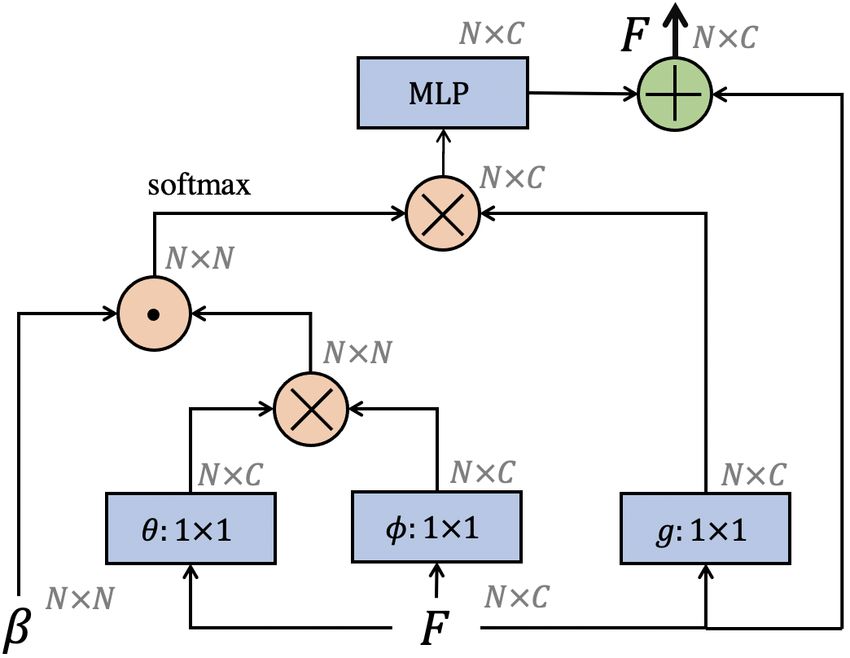
such as DGR [16] and 3DRegNet [51], formulate outlier comprehensively reviewed in [56]. Recently, learning-
rejection as an inlier/outlier classification problem, where based algorithms have been proposed to replace the indi-
the networks embed deep features from correspondence in- vidual components in the classical registration pipeline, in-
put, and predict inlier probability of each correspondence cluding keypoint detection [4, 40, 34] and feature descrip-
for outlier removal. For feature embedding, those meth- tion [21, 22, 23, 55, 4, 18, 28, 32, 2]. Besides, end-to-
ods solely rely on generic operators such as sparse con- end registration networks [3, 67, 68, 76] have been pro-
volution [17] and pointwise MLP [57] to capture the con- posed. However, their robustness and applicability in com-
textual information, while the essential 3D spatial relations plex scenes cannot always meet expectation, as observed
are omitted. Additionally, during outlier pruning, the ex- in [16], due to highly outlier-contaminated matches.
isting methods classify each correspondence only individ- Traditional outlier rejection. RANSAC [24] and its vari-
ually, again overlooking the spatial compatibility between ants [19, 5, 37, 39] are still the most popular outlier rejec-
inliers and may hinder the classification accuracy. tion methods. However, their major drawbacks are slow
All the aforementioned outlier rejection methods are convergence and low accuracy in cases with large outlier ra-
either hand-crafted with spatial consistency adopted, or tio. Such problems become more obvious in 3D point cloud
learning-based without spatial consistency integrated. In registration since the description ability of 3D descriptors is
this paper, we aim to take the best from both line of meth- generally weaker than those in 2D domain [42, 6, 44, 43, 45]
ods, and propose PointDSC, a powerful two-stage deep neu- due to the irregular density and the lack of useful tex-
ral network that explicitly leverages the spatial consistency ture [11]. Thus, geometric consistency, such as length con-
constraints during both feature embedding and outlier prun- straint under rigid transformation, becomes important and
ing. is commonly utilized by traditional outlier rejection algo-
Specifically, given the point coordinates of input corre- rithms and analyzed through spectral techniques [38, 20],
spondences, we first propose a spatial-consistency guided voting schemes [26, 74, 61], maximum clique [54, 12, 64],
nonlocal module for geometric feature embedding, which random walk [14], belief propagation [81] or game the-
captures the relations among different correspondences by ory [59]. Meanwhile, some algorithms based on BnB [11]
combining the length consistency with feature similarity to or SDP [37] are accurate but usually have high time com-
obtain more representative features. Second, we formulate plexity. Besides, FGR [82] and TEASER [70, 71] are tol-
a differentiable spectral matching module, and feed it with erant to outliers from robust cost functions such as Geman-
not only the point coordinates, but also the embedded fea- McClure function. A comprehensive review of traditional
tures to alleviate the ambiguity problem. Finally, to bet- 3D outlier rejection methods can be found in [73, 72].
ter handle the small overlap cases, we propose a seeding Learning-based outlier rejection. Learning-based out-
mechanism, which first identifies a set of reliable corre- lier rejection methods are first introduced in the 2D image
spondences, then forms several different subsets to perform matching task [48, 78, 79, 65], where outlier rejection is
the neural spectral matching multiple times. The best rigid formulated as an inlier/outlier classification problem. The
transformation is finally determined such that the geometric recent 3D outlier rejection methods DGR [16] and 3DReg-
consensus is maximized. To summarize, our main contribu- Net [51] follow this idea, and use operators such as sparse
tions are threefold: convolution [17] and pointwise MLP [57] to classify the pu-
tative correspondences. However, they both ignore the rigid
1. We propose a spatial-consistency guided nonlocal (SC- property of 3D Euclidean transformations that has been
Nonlocal) module for feature embedding, which ex- widely shown to be powerful side information. In contrast,
plicitly leverages the spatial consistency to weigh the our network explicitly incorporates the spatial consistency
feature correlation and guide the neighborhood search. between inlier correspondences, constrained by rigid trans-
2. We propose a differentiable neural spectral match- formations, for pruning the outlier correspondences.
ing (NSM) module based on traditional SM for outlier
removal, which goes beyond the simple length consis- 3. Methodology
tency metric through deep geometric features.
3. Besides showing the superior performance over the In this work, we consider two sets of sparse keypoints
state-of-the-arts, our model also demonstrates strong X ∈ R|X|×3 and Y ∈ R|Y|×3 from a pair of partially
generalization ability from indoor to outdoor scenar- overlapping 3D point clouds, with each keypoint having an
ios, and wide applicability with different descriptors. associated local descriptor. The input putative correspon-
dence set C can be generated by nearest neighbor search
2. Related Work using the local descriptors. Each correspondence ci ∈ C is
denoted as ci = (xi , yi ) ∈ R6 , where xi ∈ X, yi ∈ Y
Point cloud registration. Traditional point cloud regis- are the coordinates of a pair of 3D keypoints from the two
tration algorithms (e.g., [8, 1, 50, 33, 46, 46]) have been sets. Our objective is to find an inlier/outlier label for ci , be-
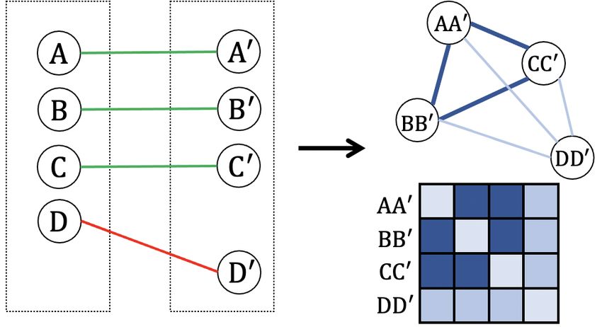
2Figure 2: Architecture of the proposed network PointDSC. It takes as input the coordinates of putative correspondences, and
outputs a rigid transformation and an inlier/outlier label for each correspondence. The Spatial Consistency Nonlocal (SC-
Nonlocal) module and the Neural Spectral Matching (NSM) module are two key components of our network, and perform
feature embedding and outlier pruning, respectively. The green lines and red lines are inliers and outliers, respectively. LS
represents least-squares fitting.
ing wi = 1 and 0, respectively, and recover an optimal 3D
rigid transformation R̂, t̂ between the two point sets. The
pipeline of our network PointDSC is shown in Fig. 2 and
can be summarized as follows:
1. We embed the input correspondences into high dimen-
sional geometric features using the SCNonlocal mod-
ule (Sec. 3.2).
2. We estimate the initial confidence vi of each corre-
spondence ci to select a limited number of highly con-
Figure 3: The spatial-consistency guided nonlocal layer. β
fident and well-distributed seeds (Sec. 3.3).
represents the spatial consistency matrix calculated using
3. For each seed, we search for its k nearest neighbors in
Eq. 2 and F is the feature from the previous layer.
the feature space and perform neural spectral match-
ing (NSM) to obtain its confidence of being an in-
lier. The confidence values are used to weigh the least- the discriminative embedding space. In the model fitting
squares fitting for computing a rigid transformation for step, our neural spectral matching module (Sec. 3.4) effec-
each seed (Sec. 3.4). tively prunes the potential outliers in the retrieved subsets,
producing a correct model even when starting from a not-
4. The best transformation matrix is selected from all the
all-inlier sample. In this way, PointDSC can tolerate large
hypotheses as the one that maximizes the number of
outlier ratios and produce highly precise registration results,
inlier correspondences (Sec. 3.5).
without needing exhaustive iterations.
3.1. PointDSC vs. RANSAC
3.2. Geometric Feature Embedding
Here, we clarify the difference between PointDSC and
RANSAC to help understand the insights behind our algo- The first module of our network is the SCNonlocal mod-
rithm. Despite not being designed for improving classic ule, which receives the correspondences C as input and pro-
RANSAC, our PointDSC shares a hypothesize-and-verify duces a geometric feature for each correspondence. Previ-
pipeline similar to RANSAC. In the sampling step, instead ous networks [16, 51] learn the feature embedding through
of randomly sampling minimal subsets iteratively, we uti- generic operators, ignoring the unique properties of 3D
lize the learned embedding space to retrieve a pool of larger rigid transformations. Instead, our SCNonlocal module ex-
correspondence subsets in one shot (Sec. 3.2 and Sec. 3.3). plicitly utilizes the spatial consistency between inlier cor-
The correspondences in such subsets have higher probabili- respondences to learn a discriminative embedding space,
ties of being inliers thanks to the highly confident seeds and where inlier correspondences are close to each other.
3As illustrated in Fig. 2, our SCNonlocal module has 12
blocks, each of which consists of a shared Perceptron layer,
a BatchNorm layer with ReLU, and the proposed nonlo-
cal layer. Fig. 3 illustrates this new nonlocal layer. Let
fi ∈ F be the intermediate feature representation for cor-
respondence ci . The design of our nonlocal layer for up-
dating the features draws inspiration from the well-known
nonlocal network [66], which captures the long-range de-
pendencies using nonlocal operators. Our contribution is to
introduce a novel spatial consistency term to complement Figure 4: (a) Inlier correspondence pairs (c1 , c2 ) always
the feature similarity in nonlocal operators. Specifically, we satisfy the length consistency, while outliers (e.g. c4 ) are
update the features using the following equation: usually not spatially consistent with either inliers (c1 , c2 )
X|C| or other outliers (e.g. c3 ). However, there exist ambigu-
fi = fi + MLP( softmaxj (αβ)g(fj )) , (1) ity when inliers (c2 ) and outliers (c3 ) happen to satisfy the
j
where g is a linear projection function. The feature similar- length consistency. The feature similarity term α provides
ity term α is defined as the embedded dot-product similar- the possibility to alleviate the ambiguity issue. (b) The cor-
ity [66]. The spatial consistency term β is defined based on respondence subsets of a seed (blue line) found by spatial
the length constraint of 3D rigid transformations, as illus- kNN (Left) and feature-space kNN (Right).
trated in Fig. 4a (c1 and c2 ).
Specifically, we compute β by measuring the length dif- apply neural spectral matching locally. We first find reliable
ference between the line segments of point pairs in X and and well-distributed correspondences as seeds, and around
its corresponding segments in Y: them search for consistent correspondences in the feature
space. Then each subset is expected to have a higher inlier
d2ij
βij = [1 − 2 ]+ , dij = kxi − xj k − kyi − yj k , (2) ratio than the input correspondence set, and is thus easier
σd for neural spectral matching to find a correct cluster.
where [·]+ is the max(·, 0) operation to ensure a non- To select the seeds, we first adopt an MLP to estimate
negative value of βij , and σd is a distance parameter (see the initial confidence vi of each correspondence using the
Sec. 4) to control the sensitivity to the length difference. feature fi learned by the SCNonlocal module, and then ap-
Correspondence pairs having the length difference larger ply Non-Maximum Suppression [42] over the confidence to
than σd are considered to be incompatible and get zero for find the well-distributed seeds. The selected seeds will be
β. In contrast, βij gives a large value only if the two corre- used to form multiple correspondence subsets for the neural
spondences ci and cj are spatially compatible, serving as a spectral matching.
reliable regulator to the feature similarity term.
Note that other forms of spatial consistency can also be 3.4. Neural Spectral Matching
easily incorporated here. However, taking an angle-based
In this step, we leverage the learned feature space to aug-
spatial consistency constraint as an example, the normals of
ment each seed with a subset of consistent correspondences
input keypoints might not always be available for outlier re-
by performing k-nearest neighbor searching in the feature
jection and the normal estimation task is challenging on its
space. We then adopt the proposed neural spectral match-
own especially for LiDAR point clouds [80]. Our SCNon-
ing (NSM) over each subset to estimate a transformation as
local module produces for each correspondence ci a feature
one hypothesis. Feature-space kNN has several advantages
representation fi , which will be used in both seed selection
over spatial kNN, as illustrated in Fig. 4b. First, the neigh-
and neural spectral matching module.
bors found in the feature space are more likely to follow a
similar transformation as the seeds, thanks to the SCNon-
3.3. Seed Selection
local module. Second, the neighbors chosen in the feature
As mentioned before, the traditional spectral matching space can be located far apart in the 3D space, leading to
technique has difficulties in finding a dominant inlier clus- more robust transformation estimation results.
ter in low overlapping cases, where it would fail to provide Given the correspondence subset C 0 ⊆ C (|C 0 | = k)
a clear separation between inliers and outliers [75]. In such of each seed constructed by kNN search, we apply NSM to
cases, directly using the output from spectral matching in estimate the inlier probability, which is subsequently used
weighted least-squares fitting [8] for transformation estima- in the weighted least-squares fitting [8] for transformation
tion may lead to a sub-optimal solution since there are still estimation. Following [38], we first construct a matrix M
many outliers not being explicitly rejected. To address this representing a compatibility graph associated with C 0 , as il-
issue, inspired by [13], we design a seeding mechanism to lustrated in Fig. 5. Instead of solely relying on the length
4by each transformation,
X|C| q
||R0 xi + t0 − yi || < τ ,
y
R̂, t̂ = arg max
0 0
(6)
R ,t i
where J·K is the Iverson bracket and τ denotes an inlier
|C|
y w ∈ R are given
threshold. The final inlier/outlier labels
by wi = J||R̂xi + t̂ − yi || < τ . We then recompute
the transformation matrix using all the surviving inliers in a
Figure 5: Constructing the compatibility graph and associ- least-squares manner, which is a common practice [19, 5].
ated matrix (Right) from the input correspondences (Left).
We set the matrix diagonal to zero following [38]. The 3.6. Loss Formulation
weight of each graph edge represents the pairwise compati-
bility between two associated correspondences. Considering the compatibility graph illustrated in Fig. 5,
previous works [16, 51] mainly adopt node-wise losses,
consistency as [38], we further incorporate the geometric which supervise each correspondence individually. In our
feature similarity to tackle the ambiguity problem as illus- work, we further design an edge-wise loss to supervise the
trated in Fig. 4a. Each entry Mij measures the compati- pairwise relations between the correspondences.
bility between correspondence ci and cj from C 0 , which is Node-wise supervision. We denote w∗ ∈ R|C| as the
defined as ground-truth inlier/outlier labels constructed by
wi∗ = J||R∗ xi + t∗ − yi || < τ ,
y
Mij = βij ∗ γij , (3) (7)
1 ¯ 2 where R∗ and t∗ are the ground-truth rotation and transla-
γij = [1 − fi − f¯j ]+ (4) tion matries, respectively. Similar to [16, 51], we first adopt
σf2
the binary cross entropy loss as the node-wise supervision
where βij is the same as in Eq. 2, f¯i and f¯j are the L2- for learning the initial confidence by
normalized feature vectors, and σf is a parameter to control Lclass = BCE(v, w∗ ), (8)
sensitivity to feature difference (see Sec. 4).
The elements of M defined above are always non- where v is the initial confidence predicted (Sec. 3.3).
negative and increase with the compatibility between corre- Edge-wise supervision We further propose the spectral
spondences. Following [38], we consider the leading eigen- matching loss as our edge-wise supervision, formulated as
vector of matrix M as the association of each correspon- 1 X ∗ 2
Lsm = (γij − γij ) , (9)
dence with a main cluster. Since this main cluster is sta- |C|2 ij
tistically formed by the inlier correspondences, it is natural where γij∗
= Jci , cj are both inliersK is the ground-truth
to interpret this association as the inlier probability. The compatibility value and γij is the estimated compatibility
higher the association to the main cluster, the higher the value based on the feature similarity defined in Eq. 4. This
probability of a correspondence being an inlier. The lead- loss supervises the relationship between each pair of cor-
ing eigenvector e ∈ Rk can be efficiently computed by the respondences, serving as a complement to the node-wise
power iteration algorithm [47]. We regard e as the inlier supervision. Our experiments (Sec. 5.4) show that the pro-
probability, since only the relative value of e matters. Fi- posed Lsm remarkably improves the performance.
nally we use the probability e as the weight to estimate the The final loss is a weighted sum of the two losses,
transformation through least-squares fitting,
X|C 0 | Ltotal = Lsm + λLclass , (10)
2
R0 , t0 = arg min ei kRxi + t − yi k . (5) where λ is a hyper-parameter to balance the two losses.
R,t i
Eq. 5 can be solved in closed form by SVD [8]. For the
sake of completeness, we provide its derivation in the sup- 4. Implementation Details
plementary 7.6. By performing such steps for each seed Training. We implement our network in PyTorch [52].
in parallel, the network produces a set of transformations Since each pair of point clouds may have different num-
{R0 , t0 } for hypothesis selection. bers of correspondences, we randomly sample 1,000 corre-
spondences from each pair to build the batched input during
3.5. Hypothesis Selection
training and set the batch size to 16 point cloud pairs. For
The final stage of PointDSC involves selecting the best NSM, we choose the neighborhood size to be k = 40. (The
hypothesis among the transformations produced by the choice of k is studied in the supplementary 7.5). We make
NSM module. The criterion for selecting the best transfor- σf learned by the network, and set σd as 10cm for indoor
mation is based on the number of correspondences satisfied scenes and 60cm for outdoor scenes, since σd has a clear
5#kept inliers
physical meaning [38]. The hyper-parameter λ is set to 3. cluding Inlier Precision (IP)= #kept matches and Inlier Re-
We optimize the network using the ADAM optimizer with call (IR)= #kept inliers
#inliers , which are particularly introduced to
an initial learning rate of 0.0001 and an exponentially de- evaluate the outlier rejection module. For RR, one registra-
cayed factor of 0.99, and train the network for 100 epochs. tion result is considered successful if the TE is less than
All the experiments are conducted on a single RTX2080 Ti 30cm and the RE is less than 15°. For a fair comparison,
graphics card. we report two sets of results by combining different outlier
Testing. During testing, we use a full correspondence set rejection algorithms with the learned descriptor FCGF [18]
as input. We adopt Non-Maximum Suppression (NMS) to and hand-crafted descriptor FPFH [60], respectively.
ensure spatial uniformity of the selected seeds, and set the Baseline methods. We first select four representative tra-
radius for NMS to be the same value as the inlier threshold ditional methods: FGR [82], SM [38], RANSAC [24], and
τ . To avoid having excessive seeds returned by NMS and GC-RANSAC [5], as well as the state-of-the-art geometry-
make the computation cost manageable, we keep at most based method TEASER [71]. For learning-based methods,
10% of the input correspondences as seeds. To improve we choose 3DRegNet [51] and DGR [16] as the baselines,
the precision of the final transformation matrix, we further since they also focus on the outlier rejection step for point
adopt a simple yet effective post-refinement stage analogous cloud registration. We also report the results of DGR with-
to iterative re-weighted least-squares [31, 7]. The detailed out RANSAC (i.e., without the so-called safeguard mech-
algorithm can be found in the supplementary 7.1. anism) to better compare the weighted least-squares solu-
tions. We carefully tune each method to achieve the best re-
5. Experiments sults on the evaluation dataset for a fair comparison. More
The following sections are organized as follows. First, details can be found in the supplementary 7.2.
we evaluate our method (PointDSC) in pairwise registration Comparisons with the state-of-the-arts. We compare
tasks on 3DMatch dataset [77] (indoor settings) with differ- our PointDSC with the baseline methods on 3DMatch.
ent descriptors, including the learned ones and hand-crafted As shown in Table 1, all the evaluation metrics are re-
ones, in Sec. 5.1. Next, we study the generalization abil- ported in two settings: input putative correspondences con-
ity of PointDSC on KITTI dataset [25] (outdoor settings) structed by FCGF (left columns) and FPFH (right columns).
using the model trained on 3DMatch in Sec. 5.2. We fur- PointDSC achieves the best Registration Recall as well as
ther evaluate PointDSC in multiway registration tasks on the lowest average TE and RE in both settings. More statis-
augmented ICL-NUIM [15] dataset in Sec. 5.3. Finally, we tics can be found in the supplementary 7.4.
conduct ablation studies to demonstrate the importance of Combination with FCGF descriptor. Compared with the
each proposed component in PointDSC. learning-based baselines, PointDSC surpasses the second
best method, i.e., DGR, by more than 9% in terms of F1
5.1. Pairwise Registration score, indicating the effectiveness of our outlier rejection al-
We follow the same evaluation protocols in 3DMatch to gorithm. Besides, although DGR is only slightly worse than
prepare training and testing data, where the test set contains PointDSC in Registration Recall, it is noteworthy that more
eight scenes with 1, 623 partially overlapped point cloud than 35% (608/1623) registration pairs are marked as fail-
fragments and their corresponding transformation matrices. ure and solved by RANSAC (safeguard mechanism). If no
We first voxel-downsample the point clouds with a 5cm safeguard mechanism is applied, DGR only achieves 86.5%
voxel size, then extract different feature descriptors to build Registration Recall.
the initial correspondence set as input. The inlier threshold Different from the conclusion in [16], our experiments
τ is set to 10cm. indicate that RANSAC still shows competitive results when
Evaluation metrics. Following DGR [16], we use three combined with a powerful descriptor FCGF. Nevertheless,
evaluation metrics, namely (1) Registration Recall (RR), the our method is about 60 times faster than RANSAC-100k
percentage of successful alignment whose rotation error and while achieving even higher Registration Recall. We also
translation error are below some thresholds, (2) Rotation report the performance of RANSAC with the proposed post-
Error (RE), and (3) Translation Error (TE). RE and TE are refinement step to clearly demonstrate the superiority of our
defined as outlier rejection module. SM and TEASER achieve slightly
Tr(R̂T R∗ ) − 1 better Inlier Precision than PointDSC, however, they have
RE(R̂) = arccos , TE(t̂) = t̂ − t∗ 2 , much lower Inlier Recall (38.36% and 68.08% vs. 86.54%
2
(11) (Ours)). We thus conclude that PointDSC achieves a better
where R∗ and t∗ denote the ground-truth rotation and trans- trade-off between precision and recall.
lation, respectively, and the average RE and TE are com- Combination with FPFH descriptor. We further evalu-
puted only on successfully registered pairs. Besides, we ate all the outlier rejection methods equipped with the tra-
also report the intermediate outlier rejection results, in- ditional descriptor, FPFH. Note that for testing learnable
6FCGF (learned descriptor) FPFH (traditional descriptor)
RR(%↑) RE(°↓) TE(cm↓) IP(%↑) IR(%↑) F1(%↑) Time(s) RR(%↑) RE(°↓) TE(cm↓) IP(%↑) IR(%↑) F1(%↑) Time(s)
FGR [82] 78.56 2.82 8.36 - - - 0.76 40.67 3.99 9.83 - - - 0.28
SM [38] 86.57 2.29 7.07 81.44 38.36 48.21 0.03 55.88 2.94 8.15 47.96 70.69 50.70 0.03
TEASER [71] 85.77 2.73 8.66 82.43 68.08 73.96 0.11 75.48 2.48 7.31 73.01 62.63 66.93 0.03
GC-RANSAC-100k [5] 92.05 2.33 7.11 64.46 93.39 75.69 0.47 67.65 2.33 6.87 48.55 69.38 56.78 0.62
RANSAC-1k [24] 86.57 3.16 9.67 76.86 77.45 76.62 0.08 40.05 5.16 13.65 51.52 34.31 39.23 0.08
RANSAC-10k 90.70 2.69 8.25 78.54 83.72 80.76 0.58 60.63 4.35 11.79 62.43 54.12 57.07 0.55
RANSAC-100k 91.50 2.49 7.54 78.38 85.30 81.43 5.50 73.57 3.55 10.04 68.18 67.40 67.47 5.24
RANSAC-100k refine 92.30 2.17 6.76 78.38 85.30 81.43 5.51 77.20 2.62 7.42 68.18 67.40 67.47 5.25
3DRegNet [51] 77.76 2.74 8.13 67.34 56.28 58.33 0.05 26.31 3.75 9.60 28.21 8.90 11.63 0.05
DGR w/o s.g. [16] 86.50 2.33 7.36 67.47 78.94 72.76 0.56 27.04 2.61 7.76 28.80 12.42 17.35 0.56
DGR [16] 91.30 2.40 7.48 67.47 78.94 72.76 1.36 69.13 3.78 10.80 28.80 12.42 17.35 2.49
PointDSC 93.28 2.06 6.55 79.10 86.54 82.35 0.09 78.50 2.07 6.57 68.57 71.61 69.85 0.09
Table 1: Registration results on 3DMatch. RANSAC-100k refine represents RANSAC with 100k iterations, followed by the
proposed post-refinement step. DGR w/o s.g. represents DGR [16] without the safeguard mechanism (RANSAC). The Time
columns report the average time cost during testing, excluding the construction of initial input correspondences.
RR(↑) RE(↓) TE(↓) F1(↑) Time Living1 Living2 Office1 Office2 AVG
SM [38] 79.64 0.47 12.15 56.37 0.18 ElasticFusion [69] 66.61 24.33 13.04 35.02 34.75
RANSAC-1k [24] 11.89 2.51 38.23 14.13 0.20 InfiniTAM [35] 46.07 73.64 113.8 105.2 84.68
RANSAC-10k 48.65 1.90 37.17 42.35 1.23 BAD-SLAM[63] fail 40.41 18.53 26.34 -
Multiway + FGR [82] 78.97 24.91 14.96 21.05 34.98
RANSAC-100k 89.37 1.22 25.88 73.13 13.7
Multiway + RANSAC [24] 110.9 19.33 14.42 17.31 40.49
DGR [16] 73.69 1.67 34.74 4.51 0.86 Multiway + DGR [16] 21.06 21.88 15.76 11.56 17.57
PointDSC 90.27 0.35 7.83 70.89 0.31 Multiway + PointDSC 20.25 15.58 13.56 11.30 15.18
DGR re-trained 77.12 1.64 33.10 27.96 0.86
PointDSC re-trained 98.20 0.35 8.13 85.54 0.31 Table 3: ATE(cm) on Augmented ICL-NUIM. The last col-
Table 2: Registration results on KITTI under FPFH setting. umn is the average ATE over all scenes. Since BAD-SLAM
fails on one scene, we do not report its average ATE.
outlier rejection methods including PointDSC, we directly
re-use the model trained with the FCGF descriptor with- We report two sets of results for DGR and PointDSC ob-
out fine-tuning, since it is expected that the outlier rejec- tained when trained from scratch (labelled “re-trained”) and
tion networks are seamlessly compatible with different fea- pre-trained on 3DMatch (no extra label). As shown in Ta-
ture descriptors. As shown in Table 1, the superiority of ble 2, PointDSC trained on 3DMatch still gives compet-
PointDSC becomes more obvious when evaluated with the itive results, demonstrating its strong generalization abil-
FPFH, where PointDSC achieves 78.5% in Registration Re- ity on the unseen dataset. When re-trained from scratch,
call and remarkably surpasses the competitors. RANSAC- PointDSC can be further improved and outperform the base-
1k and RANSAC-10k perform significantly worse since the line approaches by a significant margin.
outlier ratios are much higher when using FPFH to build
the input correspondences. RANSAC-100k with the post-
5.3. Multiway Registration
refinement step still achieves the second best performance For evaluating multiway registration, we use Augmented
at the cost of the high computation time. In summary, all ICL-NUIM dataset [15], which augments each synthetic
the other methods suffer from larger performance degrada- scene [29] with a realistic noise model. To test the general-
tion than PointDSC when equipped with a weaker descrip- ization ability, we again use the models trained on 3DMatch
tor, strongly demonstrating the robustness of PointDSC to without fine-tuning. Following [16], we first perform pair-
the input correspondences generated by different feature de- wise registration using PointDSC with FPFH descriptor to
scriptors. obtain the initial poses, then optimize the poses using pose
graph optimization [36] implemented in Open3D [83]. We
5.2. Generalization to Outdoor Scenes report the results of baseline methods presented in [16]. The
In order to evaluate the generalization of PointDSC to Absolute Trajectory Error (ATE) is reported as the evalua-
new datasets and unseen domains, we evaluate on a LiDAR tion metric. As shown in Table 3, our method achieves the
outdoor dataset, namely the KITTI odometry dataset, using lowest average ATE over three of the four tested scene types.
the model trained on 3DMatch. We follow the same data
5.4. Ablation Studies
splitting strategy in [18, 16] for a fair comparison. We use
30cm voxel size and set the inlier threshold τ to 60cm. The Ablation on feature encoder. To study the effectiveness
evaluation metrics are the same as those used in the indoor of the proposed SCNonlocal module, we conduct extensive
setting with a 60cm TE threshold and a 5° RE threshold. ablation experiments on 3DMatch. Specifically, we com-
Comparisons with the state-of-the-arts. We choose SM, pare (1) PointCN (3D version of [48], which is the feature
DGR, and RANSAC as the baseline methods, and combine extraction module adopted by 3DRegNet [51]); (2) Nonlo-
them with the FPFH descriptor. We choose FPFH because cal (the SCNonlocal module without the spatial term, i.e.,
the results with FCGF are more or less saturated. (The re- the same operator as in [66]); and (3) SCNonlocal (the pro-
sults with FCGF can be found in the supplementary 7.5.) posed operator). All the above methods are combined either
7RR(↑) RE(↓) TE(↓) F1(↑) Time
Traditional SM 86.57 2.29 7.07 48.21 0.03
+ neural 88.43 2.21 6.91 48.88 0.06
+ seeding 92.91 2.15 6.72 82.35 0.08
+ refine 93.28 2.06 6.55 82.35 0.09
w/o Lsm 92.61 2.07 6.75 81.58 0.09
Table 5: Ablation experiments of NSM module. Note that
every row with ‘+’ represents the previous row equipped
with the new component. +refine is our full model. The
last row is the full model trained without Lsm .
Figure 6: The distribution of feature similarity of inlier pairs
and non-inlier pairs (i.e. at least one outlier in the pair).
RR(↑) IP(↑) IR(↑) F1(↑) Time
PointCN + classifier 78.19 58.05 39.59 42.65 0.04
Nonlocal + classifier 83.30 65.49 67.13 64.28 0.07
SCNonlocal + classifier 88.17 74.74 77.86 75.04 0.07
PointCN + NSM 92.48 78.48 82.10 79.98 0.06
Nonlocal + NSM 92.54 78.68 83.13 80.58 0.09
SCNonlocal + NSM 93.28 79.10 86.54 82.35 0.09
Table 4: Ablation experiments of SCNonlocal module.
Rows 1-3 and Rows 4-6 show the registration results of
different feature extractors combined with a classification
layer and the neural spectral matching module, respectively.
with a classification layer [16, 51] or a proposed NSM layer,
resulting in six combinations in total. Other training or test-
ing settings remain unchanged for a fair comparison.
As shown in Table 4, the proposed SCNonlocal module
consistently improves the registration results across all the
settings and metrics. The spatial term plays a critical role in
the SCNonlocal module, without which the Nonlocal mod- Figure 7: Visualization of outlier rejection results on exam-
ule performs drastically worse. Furthermore, we compute ples with high outlier ratios from 3DMatch (first row) and
the feature similarity defined in Eq. 4 between each pair of KITTI (second row). From left to right: input correspon-
correspondences and plot the distribution in Fig. 6. With dences, results of RANSAC-100k, and results of PointDSC.
the SCNonlocal module, the similarity of the inlier pairs is
concentrated near 0.8 and is generally much larger than that qualitative results.
of the non-inlier pairs. This implies that inliers are closer
to each other in the embedding space. In contrast, for the 6. Conclusion
baseline methods, the inliers are less concentrated, i.e., the We have designed a novel 3D outlier rejection network
average similarity between inliers is low. that explicitly incorporates spatial consistency established
Ablation on spectral matching. We further conduct by Euclidean transformations. We have proposed a spatial-
ablation experiments to demonstrate the importance of consistency guided nonlocal module (SCNonlocal) and
NSM module. As shown in Table 5, the comparison be- a neural spectral matching module (NSM) for feature
tween Rows 1 and 2 shows that augmenting the traditional embedding and outlier pruning, respectively. We further
SM with neural feature consistency notably improves the proposed a seeding mechanism to adopt the NSM module
result. For +seeding, we adopt the neural spectral matching multiple times to boost the robustness under high outlier
over multiple correspondence subsets found by the feature- ratios. The extensive experiments on diverse datasets
space kNN search from highly confident seeds, and deter- showed that our method brings remarkable improvement
mine the best transformation that maximizes the geometric over the state-of-the-arts. Our method can also generalize
consensus. This significantly boosts the performance be- to unseen domains and cooperate with different local
cause it is easier to find the inlier clusters for the consistent descriptors seamlessly.
correspondence subsets.
Acknowledgements. This work is supported by Hong
5.5. Qualitative Results
Kong RGC GRF 16206819, 16203518 and Centre for Ap-
As shown in Fig. 7, PointDSC is robust to extremely high plied Computing and Interactive Media (ACIM) of School
outlier ratios. Please refer to the supplementary 7.7 for more of Creative Media, City University of Hong Kong.
8References [21] Haowen Deng, Tolga Birdal, and Slobodan Ilic. PPF-
FoldNet: Unsupervised learning of rotation invariant 3d local
[1] Dror Aiger, Niloy J Mitra, and Daniel Cohen-Or. 4-points descriptors. In ECCV, 2018. 2
congruent sets for robust pairwise surface registration. In
[22] Haowen Deng, Tolga Birdal, and Slobodan Ilic. PPFNet:
SIGGRAPH. 2008. 2
Global context aware local features for robust 3d point
[2] Sheng Ao, Qingyong Hu, Bo Yang, Andrew Markham, and matching. In CVPR, 2018. 2
Yulan Guo. SpinNet: Learning a general surface descriptor
[23] Haowen Deng, Tolga Birdal, and Slobodan Ilic. 3d local
for 3d point cloud registration. arXiv, 2020. 2
features for direct pairwise registration. In CVPR, 2019. 2
[3] Yasuhiro Aoki, Hunter Goforth, Rangaprasad Arun Srivat-
[24] Martin A. Fischler and Robert C. Bolles. Random sample
san, and Simon Lucey. PointNetLK: Robust & efficient point
consensus: a paradigm for model fitting with applications to
cloud registration using pointnet. In CVPR, 2019. 2
image analysis and automated cartography. Communications
[4] Xuyang Bai, Zixin Luo, Lei Zhou, Hongbo Fu, Long Quan, of The ACM, 1981. 2, 6, 7, 1
and Chiew-Lan Tai. D3Feat: Joint learning of dense detec- [25] Andreas Geiger, Philip Lenz, Christoph Stiller, and Raquel
tion and description of 3d local features. In CVPR, 2020. 1, Urtasun. Vision meets robotics: The kitti dataset. IJRR,
2, 3 2013. 6
[5] Daniel Barath and Jiřı́ Matas. Graph-cut ransac. In CVPR, [26] Anders Glent Buch, Yang Yang, Norbert Kruger, and Henrik
2018. 2, 5, 6, 7, 1 Gordon Petersen. In search of inliers: 3d correspondence by
[6] Herbert Bay, Tinne Tuytelaars, and Luc Van Gool. SURF: local and global voting. In CVPR, 2014. 2
Speeded up robust features. In ECCV, 2006. 2 [27] Zan Gojcic, Caifa Zhou, Jan D Wegner, Leonidas J Guibas,
[7] Per Bergström and Ove Edlund. Robust registration of point and Tolga Birdal. Learning multiview 3d point cloud regis-
sets using iteratively reweighted least squares. Computa- tration. In CVPR, 2020. 3
tional Optimization and Applications, 2014. 6, 1 [28] Zan Gojcic, Caifa Zhou, Jan D Wegner, and Andreas Wieser.
[8] Paul J Besl and Neil D McKay. Method for registration of The perfect match: 3d point cloud matching with smoothed
3-d shapes. In Sensor fusion IV: control paradigms and data densities. In CVPR, 2019. 1, 2
structures. International Society for Optics and Photonics, [29] Ankur Handa, Thomas Whelan, John McDonald, and An-
1992. 2, 4, 5 drew J Davison. A benchmark for rgb-d visual odometry, 3d
[9] JiaWang Bian, Wen-Yan Lin, Yasuyuki Matsushita, Sai-Kit reconstruction and slam. In ICRA, 2014. 7
Yeung, Tan-Dat Nguyen, and Ming-Ming Cheng. GMS: [30] Yisheng He, Wei Sun, Haibin Huang, Jianran Liu, Haoqiang
Grid-based motion statistics for fast, ultra-robust feature cor- Fan, and Jian Sun. PVN3D: A deep point-wise 3d keypoints
respondence. In CVPR, 2017. 1 voting network for 6dof pose estimation. In CVPR, 2020. 2
[10] G. Bradski. The OpenCV Library. Dr. Dobb’s Journal of [31] Paul W Holland and Roy E Welsch. Robust regression us-
Software Tools, 2000. 1 ing iteratively reweighted least-squares. Communications in
[11] Álvaro Parra Bustos and Tat-Jun Chin. Guaranteed outlier Statistics-theory and Methods, 1977. 6
removal for point cloud registration with correspondences. [32] Shengyu Huang, Zan Gojcic, Mikhail Usvyatsov, Andreas
PAMI, 2017. 2 Wieser, and Konrad Schindler. PREDATOR: Registration of
[12] Alvaro Parra Bustos, Tat-Jun Chin, Frank Neumann, Tobias 3d point clouds with low overlap. arXiv, 2020. 2
Friedrich, and Maximilian Katzmann. A practical maximum [33] Bing Jian and Baba C Vemuri. Robust point set registration
clique algorithm for matching with pairwise constraints. using gaussian mixture models. PAMI, 2010. 2
arXiv, 2019. 2 [34] Zi Jian Yew and Gim Hee Lee. 3DFeat-Net: Weakly super-
[13] Luca Cavalli, Viktor Larsson, Martin Ralf Oswald, Torsten vised local 3d features for point cloud registration. In ECCV,
Sattler, and Marc Pollefeys. AdaLAM: Revisiting hand- 2018. 1, 2
crafted outlier detection. arXiv, 2020. 1, 4 [35] Olaf Kähler, Victor A Prisacariu, and David W Murray. Real-
[14] Minsu Cho, Jungmin Lee, and Kyoung Mu Lee. Reweighted time large-scale dense 3d reconstruction with loop closure.
random walks for graph matching. In ECCV, 2010. 2 In ECCV, 2016. 7
[15] Sungjoon Choi, Qian-Yi Zhou, and Vladlen Koltun. Robust [36] Rainer Kümmerle, Giorgio Grisetti, Hauke Strasdat, Kurt
reconstruction of indoor scenes. In CVPR, 2015. 6, 7 Konolige, and Wolfram Burgard. g2o: A general framework
[16] Christopher Choy, Wei Dong, and Vladlen Koltun. Deep for graph optimization. In ICRA, 2011. 7
global registration. In CVPR, 2020. 1, 2, 3, 5, 6, 7, 8 [37] Huu M Le, Thanh-Toan Do, Tuan Hoang, and Ngai-Man
[17] Christopher Choy, JunYoung Gwak, and Silvio Savarese. 4d Cheung. SDRSAC: Semidefinite-based randomized ap-
spatio-temporal convnets: Minkowski convolutional neural proach for robust point cloud registration without correspon-
networks. In CVPR, 2019. 2 dences. In CVPR, 2019. 2
[18] Christopher Choy, Jaesik Park, and Vladlen Koltun. Fully [38] Marius Leordeanu and Martial Hebert. A spectral technique
convolutional geometric features. In ICCV, 2019. 1, 2, 6, 7 for correspondence problems using pairwise constraints. In
[19] Ondřej Chum, Jiřı́ Matas, and Josef Kittler. Locally opti- ICCV, 2005. 1, 2, 4, 5, 6, 7
mized ransac. In JPRS. Springer, 2003. 2, 5 [39] Jiayuan Li, Qingwu Hu, and Mingyao Ai. GESAC: Robust
[20] Timothee Cour, Praveen Srinivasan, and Jianbo Shi. Bal- graph enhanced sample consensus for point cloud registra-
anced graph matching. In NeurIPS, 2007. 2 tion. ISPRS, 2020. 2
9[40] Jiaxin Li and Gim Hee Lee. Usip: Unsupervised stable in- [58] Siwen Quan and Jiaqi Yang. Compatibility-guided sampling
terest point detection from 3d point clouds. In ICCV, 2019. consensus for 3-d point cloud registration. TGRS, 2020. 1
2 [59] Emanuele Rodolà, Andrea Albarelli, Filippo Bergamasco,
[41] Lei Li, Siyu Zhu, Hongbo Fu, Ping Tan, and Chiew-Lan Tai. and Andrea Torsello. A scale independent selection process
End-to-end learning local multi-view descriptors for 3d point for 3d object recognition in cluttered scenes. IJCV, 2013. 2
clouds. In CVPR, 2020. 1 [60] Radu Bogdan Rusu, Nico Blodow, and Michael Beetz. Fast
[42] David G Lowe. Distinctive image features from scale- point feature histograms (fpfh) for 3d registration. In ICRA,
invariant keypoints. IJCV, 2004. 1, 2, 4 2009. 6
[43] Zixin Luo, Tianwei Shen, Lei Zhou, Jiahui Zhang, Yao Yao, [61] Hamdi M Sahloul, Shouhei Shirafuji, and Jun Ota. An accu-
Shiwei Li, Tian Fang, and Long Quan. ContextDesc: Lo- rate and efficient voting scheme for a maximally all-inlier 3d
cal descriptor augmentation with cross-modality context. In correspondence set. PAMI, 2020. 2
CVPR, 2019. 2 [62] Paul-Edouard Sarlin, Daniel DeTone, Tomasz Malisiewicz,
[44] Zixin Luo, Tianwei Shen, Lei Zhou, Siyu Zhu, Runze Zhang, and Andrew Rabinovich. Superglue: Learning feature
Yao Yao, Tian Fang, and Long Quan. GeoDesc: Learn- matching with graph neural networks. In CVPR, 2020. 2
ing local descriptors by integrating geometry constraints. In [63] Thomas Schops, Torsten Sattler, and Marc Pollefeys. Bad
ECCV, 2018. 2 slam: Bundle adjusted direct rgb-d slam. In CVPR, 2019. 7
[45] Zixin Luo, Lei Zhou, Xuyang Bai, Hongkai Chen, Jiahui [64] Jingnan Shi, Heng Yang, and Luca Carlone. ROBIN: a
Zhang, Yao Yao, Shiwei Li, Tian Fang, and Long Quan. graph-theoretic approach to reject outliers in robust estima-
ASLFeat: Learning local features of accurate shape and lo- tion using invariants. arXiv, 2020. 2
calization. In CVPR, 2020. 2
[65] Weiwei Sun, Wei Jiang, Eduard Trulls, Andrea Tagliasacchi,
[46] Nicolas Mellado, Dror Aiger, and Niloy J Mitra. Super 4pcs
and Kwang Moo Yi. ACNe: Attentive context normalization
fast global pointcloud registration via smart indexing. In
for robust permutation-equivariant learning. In CVPR, 2020.
CGF, 2014. 2
2
[47] RV Mises and Hilda Pollaczek-Geiringer. Praktische ver-
[66] Xiaolong Wang, Ross Girshick, Abhinav Gupta, and Kaim-
fahren der gleichungsauflösung. ZAMM-Journal of Ap-
ing He. Non-local neural networks. In CVPR, 2018. 4, 7
plied Mathematics and Mechanics/Zeitschrift für Ange-
wandte Mathematik und Mechanik, 1929. 5 [67] Yue Wang and Justin M. Solomon. Deep closest point:
Learning representations for point cloud registration. In
[48] Kwang Moo Yi, Eduard Trulls, Yuki Ono, Vincent Lepetit,
ICCV, 2019. 2
Mathieu Salzmann, and Pascal Fua. Learning to find good
correspondences. In CVPR, 2018. 2, 7 [68] Yue Wang and Justin M Solomon. PRNet: Self-supervised
[49] James Munkres. Algorithms for the assignment and trans- learning for partial-to-partial registration. In NeuIPS, 2019.
portation problems. Journal of the society for industrial and 2
applied mathematics, 1957. 1 [69] Thomas Whelan, Stefan Leutenegger, R Salas-Moreno, Ben
[50] Andriy Myronenko and Xubo Song. Point set registration: Glocker, and Andrew Davison. ElasticFusion: Dense slam
Coherent point drift. PAMI, 2010. 2 without a pose graph. Robotics: Science and Systems, 2015.
7
[51] G Dias Pais, Srikumar Ramalingam, Venu Madhav Govindu,
Jacinto C Nascimento, Rama Chellappa, and Pedro Miraldo. [70] Heng Yang and Luca Carlone. A polynomial-time solu-
3DRegNet: A deep neural network for 3d point registration. tion for robust registration with extreme outlier rates. arXiv,
In CVPR, 2020. 2, 3, 5, 6, 7, 8, 1 2019. 2
[52] Adam Paszke, Sam Gross, Soumith Chintala, Gregory [71] Heng Yang, Jingnan Shi, and Luca Carlone. TEASER: Fast
Chanan, Edward Yang, Zachary DeVito, Zeming Lin, Al- and certifiable point cloud registration. arXiv, 2020. 2, 6, 7,
ban Desmaison, Luca Antiga, and Adam Lerer. Automatic 1
differentiation in pytorch. In NeurIPS-W, 2017. 5 [72] Jiaqi Yang, Ke Xian, Peng Wang, and Yanning Zhang. A
[53] Sida Peng, Yuan Liu, Qixing Huang, Xiaowei Zhou, and Hu- performance evaluation of correspondence grouping meth-
jun Bao. PVNet: Pixel-wise voting network for 6dof pose ods for 3d rigid data matching. PAMI, 2019. 1, 2
estimation. In CVPR, 2019. 2 [73] Jiaqi Yang, Ke Xian, Yang Xiao, and Zhiguo Cao. Perfor-
[54] Samunda Perera and Nick Barnes. Maximal cliques based mance evaluation of 3d correspondence grouping algorithms.
rigid body motion segmentation with a rgb-d camera. In In 3DV, 2017. 1, 2
ACCV. Springer, 2012. 2 [74] Jiaqi Yang, Yang Xiao, Zhiguo Cao, and Weidong Yang.
[55] Fabio Poiesi and Davide Boscaini. Distinctive 3d local deep Ranking 3d feature correspondences via consistency voting.
descriptors. arXiv, 2020. 2 Pattern Recognition Letters, 2019. 2
[56] François Pomerleau, Francis Colas, and Roland Siegwart. [75] Zhenpei Yang, Jeffrey Z Pan, Linjie Luo, Xiaowei Zhou,
A review of point cloud registration algorithms for mobile Kristen Grauman, and Qixing Huang. Extreme relative pose
robotics. 2015. 2 estimation for rgb-d scans via scene completion. In CVPR,
[57] Charles R Qi, Hao Su, Kaichun Mo, and Leonidas J Guibas. 2019. 4
PointNet: Deep learning on point sets for 3d classification [76] Zi Jian Yew and Gim Hee Lee. RPM-Net: Robust point
and segmentation. In CVPR, 2017. 2 matching using learned features. In CVPR, 2020. 2
10[77] Andy Zeng, Shuran Song, Matthias Nießner, Matthew
Fisher, Jianxiong Xiao, and Thomas Funkhouser. 3DMatch:
Learning local geometric descriptors from rgb-d reconstruc-
tions. In CVPR, 2017. 6
[78] Jiahui Zhang, Dawei Sun, Zixin Luo, Anbang Yao, Lei Zhou,
Tianwei Shen, Yurong Chen, Long Quan, and Hongen Liao.
OANet: Learning two-view correspondences and geometry
using order-aware network. In ICCV, 2019. 1, 2
[79] Chen Zhao, Zhiguo Cao, Chi Li, Xin Li, and Jiaqi Yang.
NM-Net: Mining reliable neighbors for robust feature corre-
spondences. In CVPR, 2019. 2
[80] Ruibin Zhao, Mingyong Pang, Caixia Liu, and Yanling
Zhang. Robust normal estimation for 3d lidar point clouds in
urban environments. Sensors, 2019. 4
[81] Lei Zhou, Siyu Zhu, Zixin Luo, Tianwei Shen, Runze Zhang,
Mingmin Zhen, Tian Fang, and Long Quan. Learning and
matching multi-view descriptors for registration of point
clouds. In ECCV, 2018. 2
[82] Qian-Yi Zhou, Jaesik Park, and Vladlen Koltun. Fast global
registration. In ECCV, 2016. 2, 6, 7, 1
[83] Qian-Yi Zhou, Jaesik Park, and Vladlen Koltun. Open3D: A
modern library for 3d data processing. arXiv, 2018. 7, 1
117. Supplementary Material We initialize e0 = 1. By iterating Eq. 12 until convergence,
we get the vector e, whose elements can take real values in
7.1. Implementation Details of PointDSC [0, 1]. In practice, we find that the power iteration algorithm
We provide additional information about the implementa- usually converges in fewer than five iterations.
tion and training details of our PointDSC. The source code Data augmentation. During training, we apply data aug-
will be made publicly available after the paper gets ac- mentation, including adding Gaussian noise with standard
cepted. deviation of 0.005, random rotation angle ∈ [0◦ , 360◦ )
Post-refinement. Alg. 1 shows the pseudo-code of our around an arbitrary axis, and random translation ∈
post-refinement step. Inspired by [7], we iteratively alter- [−0.5m, 0.5m] around each axis.
nate between weighing the correspondences and computing Hyper-parameters. The hyper-parameter σd controls the
the transformation, to improve the accuracy of the trans- sensitivity to length difference, serving as a pairwise coun-
formation matrices. The inlier threshold τ is set to 10cm terpart of the unary inlier threshold τ . The larger σd , the
and 60cm for 3DMatch and KITTI, respectively. We set the more length difference between two pairs of correspon-
maximum iteration number to 20. dences we can accommodate. It is set manually for a spe-
cific scene and kept fixed. Picking a scene-specific value of
σd is easy due to its clear physical meaning. However, σf
Algorithm 1: Post-Refinement Algorithm
controlling the sensitivity to feature difference has no clear
Input: R̂, t̂: initial transformation; X, Y physical meaning. We thus leave σf to be learned by the
Output: R̂, t̂: refined transformation. network.
Parameter: τ .
if iter < maxiter then 7.2. Implementation Detail of Baseline Methods
# Compute the residual and the inlier num.
resi = ||R̂xi +yt̂ − yi ||2 The baseline methods RANSAC [24] and FGR [82] have
wi = Jres been implemented in Open3D [83]. For GC-RANSAC [5]
Pi < τ and TEASER [71], we use the official implementations.
num = wi
# If inlier num does not change, then stop. Note that we use TEASER with reciprocal check; oth-
if ∆num = 0 then erwise, it takes an extremely long time for testing when
break the number of input correspondences becomes large. For
else DGR [16], we use its official implementation and the re-
# Compute the weighting term. leased pre-trained model. Due to the unsatisfactory results
φi = (1 + ( res i 2 −1
τ ) )
of publicly released code, we re-implement SM [38] and
# Estimate transformation. 3DRegNet [51], with the implementation details as follows.
R̂, t̂ = PN Spectral matching. Traditional spectral matching [38] uses
2
arg minR,t i φi wi kRxi + t − yi k a greedy algorithm based on a one-to-one mapping con-
iter = iter + 1 straint to discretize the leading eigenvector into the in-
else lier/outlier labels. However, the greedy algorithm often
break does not show satisfactory performance in real cases. For
example, if the input correspondences are pre-filtered by
reciprocal check, the greedy algorithm could not reject any
Calculation of M. In Sec. 3.4 of the main text, we calcu- correspondences since all of them already satisfy the one-
late the compatibility between correspondences by multi- to-one mapping constraint. The Hungarian algorithm [49]
plying the spatial consistency term and the feature similar- can also be used for discretization but provides results sim-
ity term mainly because of its simplicity and good perfor- ilar to the greedy algorithm. In our work, we simply select
mance. Other fusion schemes such as the weighted arith- 10% of the input correspondences with the highest confi-
metic average and weighted geometric average can also be dence values as the inlier set. This approach empirically
used to define the compatibility metric. We have explored shows to be effective throughout our experiments. Then the
several alternatives but found only a marginal performance transformation between two point clouds can be estimated
difference. using the selected correspondences.
Power iteration algorithm. The power iteration algorithm 3DRegNet. We keep the network architecture proposed in
can compute the leading eigenvector e of the matrix M in 3DRegNet [51] and train it on 3DMatch using the same set-
several iterations. For M ∈ Rk×k , the power iteration op- tings as PointDSC. However, as observed in [16], 3DReg-
erator is Net does not converge during training and the registration
Meiter block cannot produce reasonable results. We speculate that
eiter+1 = . (12) directly regressing the pose results in the poor performance
kMeiter k
1due to the non-linearity of the rotation space [53, 30]. Thus 7.5. Additional Experiments
we regard the output of the classification block as the in-
Registration results on KITTI. Due to the space limita-
lier confidence and use the confidence as the weight for
tion and the saturated performance under the FCGF setting,
weighted least-squares fitting. We then train the network
we only report the registration results on KITTI under the
using the classification loss only, since we find the regis-
FPFH setting in the main text. Here we report the perfor-
tration loss does not improve the performance. The modi-
mance of all the methods combined with FCGF in Table 9.
fied 3DRegNet becomes a 3D variant of PointCN [48] and
For the learning-based models DGR and PointSM, we re-
achieves reasonable results.
port the performance of the models trained from scratch (la-
belled “re-trained”) and pre-trained on the indoor dataset
7.3. Time Complexity Analysis
3DMatch (no extra label) with the FCGF descriptor.
We report the average runtime of each component in
the proposed pipeline on the 3DMatch test set (roughly RR(↑) RE(↓) TE(↓) F1(↑) Time
SM 96.76 0.50 19.73 22.84 0.10
5k putative correspondence per fragment) in Table 6. RANSAC-1k 97.12 0.48 23.37 84.26 0.22
The reported times are measured using an Intel Xeon 8- RANSAC-10k 98.02 0.41 22.94 85.05 1.43
core 2.1GHz CPU (E5-2620) and an NVIDIA GTX1080Ti RANSAC-100k 98.38 0.38 22.60 85.42 13.4
DGR 95.14 0.43 23.28 73.60 0.86
GPU. PointDSC 97.84 0.33 20.99 85.29 0.31
DGR re-trained 96.90 0.33 21.29 73.56 0.86
SCNonlocal Seed Selection NSM Post Refine Overall PointDSC re-trained 98.20 0.33 20.94 85.37 0.31
62.0 2.0 14.4 11.1 89.5 Table 9: Registration results on KITTI under the FCGF set-
Table 6: Runtime of each component in milli-seconds, av- ting. The reported time numbers do not include the con-
eraged over 1,623 test pairs of 3DMatch. The time of hy- struction of initial correspondences.
pothesis selection is included in the NSM module.
Under low-overlapping cases. Recently, Huang et. al [32]
have constructed a low-overlapping dataset 3DLoMatch
7.4. Additional Statistics from the 3DMatch benchmark to evaluate the point cloud
registration algorithms under low-overlapping scenarios.
We report the area under cumulative error curve (AUC) To demonstrate the robustness of our PointDSC, we fur-
of the rotation and translation errors defined in Eq. 11 at ther evaluate our method on 3DLoMatch dataset and re-
different thresholds, as shown in Table 7. PointDSC consis- port the results1 in Table 10. Note that we directly use
tently outperforms the state-of-the-arts on both the AUC of the model trained on 3DMatch without fine-tuning and keep
the Rotation Error (RE) and Translation Error (TE). 5cm voxel for FCGF descriptor. All the other settings are
the same with [32] for a fair comparison.
RE AUC TE AUC
5◦ 10◦ 15◦ 5cm 10cm 15cm 20cm 25cm 30cm
SM 50.14 67.24 74.37 16.29 35.98 48.61 56.90 62.57 66.67 5000 2500 1000 500 250 ∆
DGR 50.22 69.98 77.78 14.13 35.28 49.32 58.50 64.74 69.19 FCGF[18] + RANSAC 35.7 34.9 33.4 31.3 24.4 -
RANSAC 49.99 70.43 78.31 12.16 33.15 47.99 57.81 64.33 68.95 FCGF[18] + PointDSC 52.0 51.0 45.2 37.7 27.5 +10.74
GC-RANSAC 52.81 71.56 78.90 15.33 36.77 50.94 59.95 65.94 70.19
Predator[32] + RANSAC 54.2 55.8 56.7 56.1 50.7 -
PointDSC 57.32 74.85 81.50 17.85 40.63 54.56 63.32 69.02 73.00
Predator[32] + PointDSC 61.5 60.2 58.5 55.4 50.4 +2.50
Table 7: Registration results on 3DMatch. We calculate the
Table 10: Registration recall on the 3DLoMatch dataset us-
exact AUC following [62]: the higher, the better. We run
ing different numbers of points to construct the input cor-
100k iterations for both RANSAC and GC-RANSAC.
respondence set. The last column is the average increase
brought by PointDSC.
We also report the scene-wise registration results of our
method on 3DMatch in Table 8. As shown in Table 10, our method consistently outper-
forms RANSAC when combined with different descriptors.
RR(%) RE(°) TE(cm) IP(%) IR(%) F1(%) Moreover, our method can further boost the performance of
Kitchen 98.81 1.67 5.12 80.57 88.83 84.26
Home1 97.44 1.87 6.45 83.34 88.91 85.88
Predator [32], a recently proposed learning-based descrip-
Home2 82.21 3.36 7.46 71.39 80.20 74.78 tors especially designed for low-overlapping registration,
Hotel1 98.67 1.88 6.04 83.96 91.48 87.38 showing the effectiveness and robustness of our method un-
Hotel2 92.31 1.98 5.74 81.07 86.97 83.82 der high outlier ratios. PointDSC increases the registration
Hotel3 92.59 2.00 5.87 82.65 88.57 85.03
Study 89.04 2.29 9.20 77.00 83.72 79.97
recall by 16.3% and 7.3% under 5000 points setting for
Lab 80.52 1.91 8.41 70.31 77.88 73.46 FCGF and Predator, respectively. Note that PointDSC does
Table 8: Scene-wise statistics for PointDSC on 3DMatch. 1 The computation of registration recall is slightly different with ours,
we refer readers to [32] for more details.
2You can also read