Poisson Subsampled Renyi Differential Privacy - Proceedings of ...
←
→
Page content transcription
If your browser does not render page correctly, please read the page content below
Poisson Subsampled Renyi Differential Privacy

                                             Yuqing Zhu 1 Yu-Xiang Wang 1

                         Abstract                                2016) for differentially private deep learning. NoisySGD
                                                                 iteratively updates the model parameters as follows:
     We consider the problem of "privacy-
                                                                                            !                    #
     amplification by subsampling” under the                                                  "
     Renyi Differential Privacy (RDP) framework                              θt+1 ← θt − ηt       ∇fi (θt ) + Zt       (1)
     (Mironov, 2017). This is the main workhorse                                                i∈I
     underlying the moments accountant approach                  where θt is the model parameter at tth step, ηt is the learn-
     for differentially private deep learning (Abadi             ing rate, fi is the loss function of data point i, ∇ is the stan-
     et al., 2016). Complementing a recent result                dard gradient operator, I ⊂ [n] is a randomly subsampled
     on this problem that deals with “Sampling                   index set and Zt ∼ N (0, σ 2 I). When ∇fi (θt ) is bounded
     without Replacement” (Wang et al., 2019), we                (or clipped) in ℓ2 -norm, the Gaussian noise-adding proce-
     address the “Poisson subsampling” scheme                    dure is known to ensure (ϵ, δ)-DP for this iteration. ϵ, δ
     which selects each data point independently with            are nonnegative numbers that quantifies the privacy loss in-
     probability γ. The seemingly minor change                   curred from running the algorithm (the smaller the better).
     allows us to more precisely characterize the RDP            But this is clearly not good enough as it takes many itera-
     of M ◦ PoissonSample. In particular, we prove               tions to learn the model, and the privacy guarantee deterio-
     an exact analytical formula for the case when               rates as the algorithm continues. This is where the “privacy-
     M is the Gaussian mechanism or the Laplace                  amplification” and RDP become useful.
     mechanism. For general M, we prove an upper
     bound that is optimal up to an additive constant            The principle of “privacy-amplification by subsampling”
     of log(3)/(α − 1) and a multiplicative factor of            works seamlessly with NoisySGD as it allows us to exploit
     1 + O(γ). Our result is the first of its kind that          the randomness in choosing the minibatch I for the interest
     makes the moments accountant technique (Abadi               of a stronger privacy guarantee. Roughly speaking, if the
     et al., 2016) efficient and generally applicable for        minibatch I is obtained by selecting each data point with
     all Poisson-subsampled mechanisms. An open                  probability γ, then we can “amplify” the privacy guarantee
     source implementation is available at https:                to a stronger (O(γϵ), γδ)-DP.
     //github.com/yuxiangw/autodp.                               The RDP framework provides a complementary set of ben-
                                                                 efits that reduce the overall privacy loss over the multi-
                                                                 ple iterations we run NoisySGD. Notice that the vanilla
1. Introduction                                                  “strong-composition” is stated for any (ϵ, δ)-DP algorithm.
“Privacy-amplification by Subsampling” and the Renyi Dif-        By using the moments accountant techniques (Abadi et al.,
ferential Privacy are the two fundamental techniques that        2016) that keep track of the RDP of a specific algorithm
have been driving many exciting recent advances in dif-          — subsampled-Gaussian mechanism, one can hope to more
ferentially private learning (Abadi et al., 2016; Park et al.,   efficiently use the privacy budget than what an optimal algo-
2016; Papernot et al., 2018; McMahan et al., 2018).              rithm would be able to using only (ϵ, δ)-DP (Kairouz et al.,
                                                                 2015).
One prominent use case of both techniques is the
NoisySGD algorithm (Song et al., 2013; Bassily et al.,           In general, however, calculating the RDP for the procedure
2014; Wang et al., 2015; Foulds et al., 2016; Abadi et al.,      that first subsamples the data set then apply a randomized
                                                                 mechanism M is highly non-trivial. An exact analytical
   1
     UC Santa Barbara, Department of Computer Science. Cor-      formula is not known even for the widely-used subsampled-
respondence to: Yuqing Zhu , Yu-Xiang        Gaussian mechanism. Existing asymptotic bounds are typi-
Wang .                                     cally off by a constant, and only apply to a restricted subset
Proceedings of the 36 th International Conference on Machine     of the parameter regimes. To get the most mileage out of
Learning, Long Beach, California, PMLR 97, 2019. Copyright       the moments accountant, practitioners often resort to nu-
2019 by the author(s).                                           merical integration which calculates and keep track of a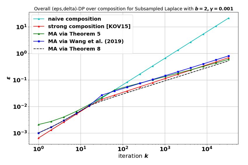
Poission Subsampled RDP

fixed list of RDP values (Abadi et al., 2016; Park et al.,               casing the use of these bounds in moments accountant-
2016).                                                                   based strong composition.
Wang et al. (2019) took a first stab at this problem and
provided a general “RDP-amplification” bound that applies         2. Background and Problem Setup
to any M. Their result, however, is still a constant fac-
tor away from being optimal. A more subtle difference             In this section, we provide some background on differential
is that Wang et al. (2019) considered “Subsampling with-          privacy, privacy-amplification by subsampling, RDP and
out Replacements” — finding a random subset of size m             the moments accountant technique so as to formally set up
at random — rather than the “Poisson subsampling” that            the problem. We will also introduce symbols and notations
was used by Abadi et al. (2016), which includes each data         as we proceed.
points independently at random with probability γ. The dif-
                                                                  Differential Privacy. Let X be the space of all data
ference is substantial enough that it introduces several new
                                                                  sets. One representation of such a data set is to take
technical hurdles.
                                                                  X = {0, 1}N where N is the size of the population and
In this paper, we provide the first general result of “privacy-   each X ∈ X is an indicator vector that describes each indi-
amplification” of RDP via Poisson subsampling. Our main           vidual’s participation in the data set. We say X, X ′ ∈ X are
contributions are the following.                                  neighbors if X ′ can be constructed by adding or removing
                                                                  one individual from X, or equivalently, ∥X − X ′ ∥1 = 1.
 1. First, we prove a nearly optimal upper bound on the           Definition 1 (Differential Privacy (Dwork et al., 2006)). A
    RDP of M ◦ PoissonSample as a function of the sam-            randomized algorithm M : X → Θ is (ϵ, δ)-DP (differ-
    pling probability γ, RDP order α, and the RDP of M            entially private) if for every pair of neighboring datasets
    up to α. The bound matches a lower bound up to an             X, X ′ ∈ X , and every possible (measurable) output set
    additive factor of log(3)/(α − 1), where α is the order       E ⊆ Θ the following inequality holds: Pr[M(X) ∈ E] ≤
    of RDP. When α is small relative to 1/γ with γ being          eϵ Pr[M(X ′ ) ∈ E] + δ.
    the sampling probability, our upper bound is optimal
                                                                  The definition places an information-theoretic limit on an
    up to a multiplicative factor of 1 + O(γαeϵ(α) ). The
                                                                  adversary’s ability to infer whether the input dataset is X
    result tightens and generalizes Lemma 3 of (Abadi
                                                                  or X ′ , and as a result, guarantees a degree of plausible de-
    et al., 2016), which addresses only the case when M
                                                                  niability to any individual in the population. ϵ, δ are pri-
    is Gaussian mechanism and applies only to the cases
                                                                  vacy loss parameters that quantify the strength of privacy
    when γ is very small.
                                                                  protection. In practice, we consider the privacy guarantee
                                                                  marginally meaningful if ϵ ≈ 1 and δ = o(1/n)1 , where n
 2. Second, we identify a novel condition on the odd order
                                                                  denotes the size of data set and o(·) is the standard little-o
    Pearson-Vajda χα -Divergences under which we can
                                                                  notation. When δ = 0, we say that M obeys ϵ-(pure) DP.
    exactly attain the lower bound. We show that Gaus-
    sian mechanism and Laplace mechanism fall under               One important property of DP relevant to this paper is
    this category, but there exists M that samples from           that it composes gracefully over multiple access. Roughly
    an exponential family distribution where the condition        speaking, if we run k sequentially chosen (ϵ, δ)-DP algo-
    is false and the lower bound is not attainable. Practi-       rithm
                                                                      √ on a dataset, the overall composed privacy loss is
    cally, our analytical characterization simplifies the mo-     (Õ( kϵ), kδ + δ ′ )-DP where the Õ notation hides loga-
    ments accountant approach for differentially private          rithmic terms in k, 1/δ and 1/δ ′ . Part of the reason for
    deep learning by avoiding numerical integration and           writing this paper is to enable sharper algorithm-dependent
    pre-specifying a list of moments. On the theory front,        composition for a popular class of algorithms that subsam-
    our result corroborates the observation of Wang et al.        ples the data first. Before we get there, let us describe the
    (2019) that the Pearson-Vajda Divergences are natural         RDP framework and the moments accountant that the make
    quantities for understanding the subsampling in differ-       these algorithm-dependent composition possible.
    ential privacy.
                                                                  Renyi Differential Privacy and Moments Accountant.
                                                                  Renyi differential privacy (RDP) is a refinement of DP that
 3. Lastly, knowing that exactly evaluating the analytical
                                                                  uses Renyi-divergence as a distance metric in the place of
    subsampled RDP bound of αth order takes α calls of
                                                                  the sup-divergence.
    the RDP subroutine ϵM (·), we propose an efficiently
    τ -term approximation scheme that uses only τ call of         Definition 2 (Rényi Differential Privacy (Mironov, 2017)).
    ϵM (·). We conduct numerical experiments to com-                 1
                                                                       It is traditionally required that δ to be cryptographically small,
    pare our general bounds, tight bound, and τ -term ap-         e.g., o(poly(1/n)), but in practice, with a big data set, δ = 1/n2
    proximations for a variety of problem setup and show-         is typically considered acceptable.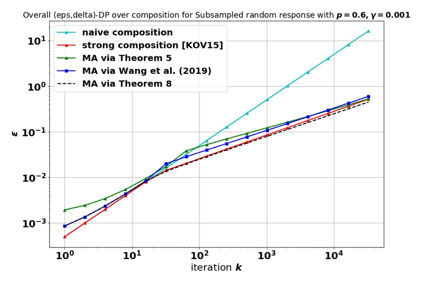
Poission Subsampled RDP

Figure 1. Illustration of the subsampled-mechanism and the key underlying idea that enables “privacy-amplification”. The diagram on
the left illustrate the two parts of randomization. Part (1): PoissonSample: Each person toss a random coin to select whether they are
included in the data set; Part (2): The subsampled data set is analyzed by a randomized algorithm M. The figure on the right illustrates
the fact that the distribution of output is a mixture distribution indexed by the different potential subset selected by the subsampling,
and that when we change the original data set by adding or removing one person, only a small fraction of the mixture components that
happen to be affected by that change will be different, hus opening up the possibility of “privacy amplifying”.

We say that a mechanism M is (α, ϵ)-RDP with order α ∈                As a side note, the initial moments accountant (Abadi et al.,
(1, ∞) if for all neighboring datasets X, X ′                         2016) keeps track of a vector of log-moment (equivalent to
                                                                      RDP up to a rescaling) associated with a pre-defined list of
        Dα (M(X)∥M(X ′ ))                                             order αs. Wang et al. (2019) observes that these optimiza-
                            $%              &α '
         1                     pM(X) (θ)                              tion problems are unimodal and proposes an analytical mo-
     :=      log Eθ∼M(X ′ )                      ≤ ϵ.
        α−1                    pM(X ′ ) (θ)                           ments accountant that solves (2) and (3) using bisections
                                                                      can be solved using bisection with a doubling trick. This
In this paper, we do not treat each α in isolation but instead        avoids the need to pre-define the list of moments to track.
take a functional view of RDP where we use ϵM (α) to de-              Wang et al. (2019) also observes that (α − 1)ϵ(α) is a con-
note that randomized algorithm M obeys (α, ϵM (α))-RDP.               vex function in α and any such discretization scheme (e.g.,
The function ϵM (·) can be viewed as a more elaborate de-             all integer α) can be extended into a continuous function in
scription of the privacy loss incurred by running M. It               α by simply doing linear interpolation.
subsumes pure-DP as an RDP algorithm is ϵ(+∞)-DP.                     Privacy amplification by subsampling. As we discussed
The moments accountant technique (Abadi et al., 2016) can             in the introduction, “privacy amplification by subsampling”
be thought of as a data structure that keeps track of the RDP         is the other workhorse (besides RDP / moments accoun-
(function) for the sequence of data accesses. Composition             tant) that drove much of the recent advances in differen-
is trivial in RDP as                                                  tially private deep learning. We would like to add that, it
                                                                      was also used as a key technical hammer for analyzing DP
              ϵM1 ×M2 (·) = [ϵM1 + ϵM2 ](·).                          algorithms for empirical risk minimization (Bassily et al.,
                                                                      2014) and Bayesian learning (Wang et al., 2015), as well as
At any given time, let the composition of all algorithms
                                                                      for studying learning-theoretic questions with differential
being M, the moments accountant can be used to produce
                                                                      privacy constraints (Kasiviswanathan et al., 2011; Beimel
an (ϵ, δ)-DP certificate using
                                                                      et al., 2013; Bun et al., 2015; Wang et al., 2016).
                             log(1/δ)
   δ⇒ϵ:           ϵ(δ) = min          + ϵM (α − 1),           (2)     We now furnish a bit more details on this central property
                          α>1  α−1                                    and highlight some subtleties in the types. The privacy am-
   ϵ⇒δ:           δ(ϵ) = min e(α−1)(ϵM (α−1)−ϵ) .             (3)     plification lemma was derived in (Kasiviswanathan et al.,
                          α>1
                                                                      2011; Beimel et al., 2013; Li et al., 2012), where all three
This approach is simpler and often produces more favor-               authors adopted what Balle et al. (2018) calls Poisson sub-
able composed privacy parameters than the advanced com-               sampling:
position approach for (ϵ, δ)-DP. As the moments accoun-
tant gain popularity, many classes of randomized algo-                Definition 3 (PoissonSample). Given a dataset X, the
rithms with exact analytical RDP are becoming available,              procedure PoissonSample outputs a subset of the data
e.g., the exponential family mechanisms (Geumlek et al.,              {xi |σi = 1, i ∈ [n]} by sampling σi ∼ Ber(γ) indepen-
2017).                                                                dently for i = 1, ..., n.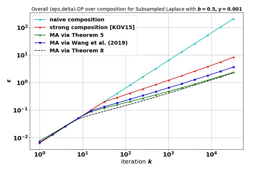
Poission Subsampled RDP

The procedure is equivalent to the “sampling without re-              As we will see in the our results, the third difference brings
placement” scheme with m ∼ Binomial(γ, n). At the limit               about some major technical challenges.
of n → ∞, γ → 0 while γn → λ, the Binomial distribu-
                                                                      Finally, Bun et al. (2018) studies subsampling in CDP with
tion converges to a Poisson distribution with parameter λ.
                                                                      a conclusion that subsampling does not amplify the CDP
This is probably the reason why it is called Poisson sam-
                                                                      parameters in general. A truncated version of CDP was
pling to begin with2 .
                                                                      then proposed, called tCDP, which does get amplified up
Here we cite the tight privacy amplification bound for                to a threshold. CDP and tCDP are closely related to RDP
PoissonSample as it first appears.                                    in that they are linear upper bounds of ϵ(α) on (1, ∞] and
                                                                      on (1, τ ] for some threshold τ respectively. RDP captures
Lemma 4 ((Li et al., 2012, Theorem 1) ). If M is (ϵ, δ)-DP,
                                                                      finer information about the underlying mechanism. The ex-
then M′ that applies
             (       M◦PoissonSample
                            )            obeys (ϵ′ , δ ′ )-DP
                                                                      perimental results in (Wang et al., 2019) suggest that unlike
with ϵ′ = log 1 + γ(eϵ − 1) and δ ′ = γδ.
                                                                      the case for the Gaussian mechanism (in which case CDP
The lemma implies that if the base privacy loss ϵ ≤ 1, then           is tight), there isn’t a good linear approximation of ϵ(α) for
the amplified privacy loss obeys that ϵ′ ≤ 2γϵ.                       the subsampled-Gaussian mechanism due to the phase tran-
                                                                      sition. Our results on the Poisson-sampling model echoes
Poisson subsampling is different from the “sampling with-             the same phenomenon.
out replacement” scheme that outputs a subset with size
γn uniformly at random. Interestingly, it was shown that              More symbols and notations. We end the section with a
the latter also enjoys the same bound with respect to the             quick summary of the notations that we introduced. X, X ′
“replace-one” version of the DP definition. In general, we            denotes two neighboring datasets. M is a randomized algo-
find that the “add/remove” version of the DP definition               rithm and ϵM (·) is the RDP function of M (the subscript
works more naturally with Poisson sampling, while the                 may be dropped when it’s clear from the context). n, m are
“replace-one” version works well with “sampling without               reserved for the size of the original and subsampled data.
replacement”. We defer a more comprehensive account of                We note that neither is public and m is random. Greek
the subsampling lemma for (ϵ, δ)-DP to (Balle & Wang,                 letters α, γ, ϵ, δ are reserved for the order of RDP, the sam-
2018) and the references therein.                                     pling probability as well as the two privacy loss parameters.
                                                                      M ◦ PoissonSample(X) is used to mean the composition
Subsampled RDP and friends. A small body of recent                    function M(PoissonSample(X)).
work focuses on deriving algorithm-specific subsampling
Lemma so that this classical wisdom can be combined with              Let us also define a few shorthands. We will denote p to
more modern techniques such as RDP and Concentrated                   be the density function of M ◦ PoissonSample(X), and q
DIfferential privacy (CDP) (Bun & Steinke, 2016) (also                to be the density from data set M ◦ PoissonSample(X ′ ).
(Dwork & Rothblum, 2016)). Abadi et al. (2016) obtains                Similarly, we will define µ0 and µ1 as two generic density
the first such results for subsampled-Gaussian mechanism              functions of M(X) and M(X ′ ).
under Poisson subsampling. Wang et al. (2019) provides a
general subsampled RDP bound that supports any M but                  3. Main results
under the “sampling without replacement” scheme. The ob-
jective of this paper is to come up with results of a similar         Before we present our main result, we would like to warn
flavor for the Poisson sampling scheme. The main differ-              the readers that the presented bounds might not be as in-
ences in our setting include:                                         terpretable. We argue that this is a feature rather than an
                                                                      artifact of our proof because we need the messiness to state
                                                                      the bound exactly. These bounds are meant to be imple-
 (a) Poisson sampling goes naturally with add/remove ver-             mented to achieve the tightest possible privacy composition
     sion of the DP definition, which is independent to the           numerically in the Moments Accountant, rather than being
     size of the data.                                                made easily interpretable. After all, “constant matters in
 (b) The size of the random subset m itself is a Binomial             differential privacy!” For the interest of interpretability, we
     random variable.                                                 provide figures that demonstrate the behaviors of the bound
                                                                      for prototypical mechanisms in practice.
 (c) It is asymmetric, the Renyi divergence of P against Q
     is different from the Renyi divergence of Q against P .
   2
     We noticed that the original definition of Poisson sampling in
the survey sampling theory is slightly more general. It allows
a different probability of sampling each person (Särndal et al.,
2003). Our results apply trivially to that setting as well with a     Theorem 5 (General upper bound). Let M be any random-
personalized RDP bound for individual i that depends on γi .          ized algorithm that obeys (α, ϵ(α))-RDP. Let γ be the sub-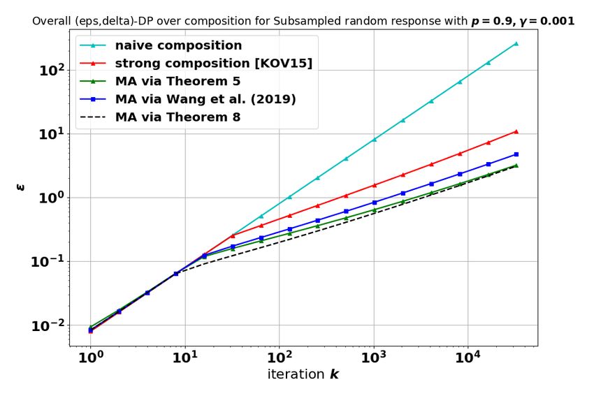
Poission Subsampled RDP

sampling probability and then we have for integer α ≥ 2,            Remark 7 (Nearly optimal Moment Accountant). This im-
                               !                                    plies that if any algorithm with the help of an oracle that
                        1                                           calculates the exact RDP for M is able to prove an (ϵ, δ)-
ϵM◦PoissonSample (α) ≤      log (1 − γ)α−1 (αγ − γ + 1)
                       α−1                                          DP for the Poisson subsampled RDP mechanism, then the
   " #                            "   #                          %
    α 2
                                α
                                $   α                               RDP upper bound we construct using Theorem 5 will lead
 +       γ (1 − γ)α−2 eϵ(2) + 3         (1 − γ)α−ℓ γ ℓ e(ℓ−1)ϵ(ℓ) .
    2                               ℓ                               to an (ϵ, 3δ)-DP bound for the same mechanism.
                               ℓ=3

                                                                    Moreover, we show that for many randomized algorithms
The proof is revealing but technically involved. One main           (including the popular Gaussian mechanism and Laplace
difference from Wang et al. (2019) is that in Poisson sam-          mechanism) that satisfy an additional assumption, we can
pling we need to bound both Dα (p∥q) and Dα (q∥p). Ex-              strengthen the upper bound further and exactly match the
isting arguments via the quasi-convexity of Renyi diver-            lower bound for all α.
gence allows us to easily bound Dα (p∥q) tightly using
                                                                    Theorem 8 (Tight upper bound). Let M be a randomized
RDP for the case when p has one more data points than
                                                                    algorithm with up to αth order RDP ϵ(α) < ∞. If for all
q, but Dα (q∥p) turns out to be very tricky. A big part of
                                                                    adjacent data sets X ∼ X ′ , and all odd 3 ≤ ℓ ≤ α,
our novelty in the proof is about analyzing Dα (q∥p). We
defer more details of the proof to Appendix A.                                                          %              &ℓ
                                                                                                           M(X)
Theorem 6 (Lower bound). M and pairs of adjacent data                Dχℓ (M(X)∥M(X ′ )) := EM(X ′ )                − 1    ≥ 0,
                                                                                                          M(X ′ )
sets such that                                                                                                             (4)
                                   *                                then the lower bound in Theorem 6 is also an upper bound.
                          1
ϵM◦PoissonSample (α) ≥         log (1 − γ)α−1 (αγ − γ + 1)
                        α−1                                  The proof of this theorem is presented in Appendix A
   " α % &                            +
          α                                                  In the theorem, M(X      M(X)
                                                                                             − 1 is a linearized ver-
 +           (1 − γ)α−ℓ γ ℓ e(ℓ−1)ϵ(ℓ) .                                                  ′)
          ℓ                                                                                                   M(X)
    ℓ=2                                                      sion of the privacy random variable log M(X          ′) and
                                                             Dχℓ (M(X)∥M(X ′ )) is the Pearson-Vajda χℓ pseudo-
Proof. The construction effectively follows Proposition 11
                                                             divergence (Vajda, 1973), which has more recently been
of (Wang et al., 2019), while adjusting for the details. Let
                                                             used to approximate any f -divergence in (Nielsen & Nock,
, be Laplace noise adding of a counting query f (X
                                                        ′
M                                                         )=
                                                             2014). The related |χℓ | version of this divergence is iden-
   x∈X ′ 1[x > 0]. Let everyone in the data set X obeys
                                                    ′
                                                             tified as the key quantity natural for studying subsampling
that x < 0. In the adjacent dataset X ′ = X ∪ {xn+1 } with
                                                             without replacement (Wang et al., 2019).
xn+1 > 0. Let µ0 be the Laplace distribution centered at
0, µ1 be the one that is centered at 1. Then we know that    The non-negativity condition requires, roughly speaking,
M(X ′ ) ∼ µ0 = q and M(X) (1 − γ)µ0 + γµ1 = p. It            the distribution of the linearized privacy loss random vari-
                                                                   M(X)
follows that                                                 able M(X    ′ ) − 1 to be skewed to the right.

         Eq [(p/q)α ] = Eµ0 [((1 − γ) + γµ1 /µ0 ) ]
                                                       α            The following Lemma provides one way to think about it.
         "α % &                                                     Lemma 9. Let π, µ be two measures that are absolute con-
               α
       =          (1 − γ)α−ℓ γ ℓ Eµ0 [(µ1 /µ0 )ℓ ].                 tinuous w.r.t. each other and let α ≥ 1.
                ℓ
          ℓ=0
                                                                    Eµ [(π/µ − 1)α ] = Eπ [(π/µ − 1)α−1 ] − Eµ [(π/µ − 1)α−1 ].
By definition Eµ0 [(µ1 /µ0 ) ] = e
                           ℓ
                                               . which the
                                   (ℓ−1)Dℓ (µ0 ∥µ1 )

RDP bonud ϵ(ℓ) is attained by µ0 , µ1 , then we have con-           Proof. Eµ [(π/µ − 1)α ] = Eµ [(π/µ − 1)(π/µ − 1)α−1 ] =
structed one pair of p, q, which implies a lower bound for          Eπ [(π/µ − 1)α−1 ] − Eµ [(π/µ − 1)α−1 ]
RDP of M ◦ PoissonSample.
                                                                    The lemma implies that (4) holds if an only if for all even
Note that the only difference between the upper and lower           2≤ℓ≤α
bounds are a factor of 3 on the third summand in side the                   %              &ℓ              %               &ℓ
logarithm. In the regime when γαeϵ(α) ≪ 1 (in which                           M(X)                           M(X)
                                                                     EM(X)             − 1     ≥ E M(X ) ′            −  1
case the third summand is much smaller than the second),                      M(X ′ )                        M(X ′ )
the upper and lower bound match up to a multiplicative fac-
                                                                    for all pairs of X, X ′ .
tor of 1 + O(γαeϵ(α) ). In all other regimes, the upper and
lower bounds match up to an additive factor of log(3)
                                                  α−1 . The
                                                                    This should intuitively be true for most mechanisms be-
                                                                                                            M(X)
results suggest that we can construct a nearly optimal mo-          cause we know from nonnegativity that M(X    ′ ) − 1 ≥ −1,

ment accountant.                                                    which poses a hard limit to which you can be skewed to the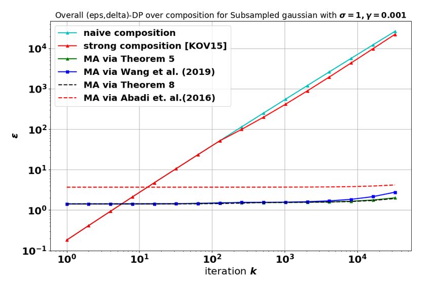
Poission Subsampled RDP

                                                                 Theorem 6 (therefore Theorem 8) can be bounded by
                                                                                           1        -
                                                                 ϵM◦PoissonSample (α) ≤          log (1 − γ)α (1 − e−ϵ(α−τ ) )
                                                                                        α−1
                                                                  + e−ϵ(α−τ ) (1 − γ + γeϵ(α−τ ) )α
                                                                    "τ % &
                                                                          α
                                                                  −           (1 − γ)α−ℓ γ ℓ (e(ℓ−1)ϵ(α−τ ) − e(ℓ−1)ϵ(ℓ) )
                                                                          ℓ
                                                                    ℓ=2
                                                                      " α     % &                                              .
                                                                                α
                                                                  +                (1 − γ)α−ℓ γ ℓ (e(ℓ−1)ϵ(ℓ) − e(ℓ−1)ϵ(α−τ ) ) .
                                                                                ℓ
                                                                    ℓ=α−τ +1
   Figure 2. Negative χα divergence in Poisson distribution.
                                                                 A similar bound can be stated for the general upper bound
                                                                 in Theorem 5, which we defer to Appendix C.
                                                                 Remark 12 (Numerical stability). The bounds in Theo-
left. Indeed, we can show that the condition is true for the     rem 5 and 8 can be written as the log − sum − exp form,
two most widely used DP procedure.                               i.e., softmax. The numerically stable way of evaluating
                                                                 log − sum − exp is well-known. The bound in Theorem 11,
Proposition 10. Condition (4) is true when M is the Gaus-        though, have both positive terms and negative terms. We
sian mechanism and Laplace mechanism.                            choose to represent the summands in the log term by a sign,
                                                                 and the logarithm of its magnitude. This makes it possible
                                                                 for us to use log − diff − exp and compute the bound in a
The proof, given in Appendix B, is interesting and can be        numerically stable way.
used as recipes to qualify other mechanisms for the tight
bound. The main difficulty of checking this condition is
in searching all pairs of neighboring data sets and identify     4. Experiments and Discussion
one pair that minimizes the odd order moment. The con-
                                                                 In this section, we conduct various numerical experiments
venient property of noise-adding procedure is that typically
                                                                 to illustrate the behaviors of the RDP for subsampled mech-
the search reduces to a univariate optimization problem of
                                                                 anisms and showcasing its usage in moments accountant
the sensitivity parameter.
                                                                 for composition. We will have three set of experiments. (1)
One may ask, whether the condition is true in general            We will just plot our RDP bounds (Theorem 5, Theorem 6)
for any randomized algorithm M? The answer is unfor-             as a function of α. (2) We will compare how close the τ -
tunately no. For example, Nielsen & Nock (2014) con-             term approximations approximate the actual bound.(5) (3)
structed an example of two Poisson distributions with neg-       We will build our moments accountant and illustrate the
ative χ3 -divergence (see Figure 2 for an illustration.) This    stronger composition that we get out of our tight bound.
also implies that for some M, we can derive a lower bound        Specifically, for each of the experiments above, we repli-
that is greater than that in Theorem 6 by simply toggling        cate the experimental setup of which takes the base mecha-
the order of X and X ′ . As a result, if one needs to work       nism M to be Gaussian mechanism, Laplace mechanism
out the tight bound, the condition needs to be checked for       and Randomized Response mechanism. Their RDP for-
each M separately.                                               mula are worked out analytically (Mironov, 2017) below:
                                                                                    α
                                                                 ϵGaussian(α) =         ,
Finally, we address the computational issue of implement-                          2σ 2
ing our bounds in moments accountant. Naive implementa-            ϵLaplace(α)   =
                                                                                     1
                                                                                          log((
                                                                                                  α      α−1
                                                                                                       )e b + (
                                                                                                                  α−1     −α
                                                                                                                        )e b for α > 1,
                                                                                   α−1          2α − 1           2α − 1
tion of Theorem 5 will easily suffer from overflow or under-
                                                                                     1
flow and it takes α calls to the RDP oracle ϵM (·) before we
                                                                                                α       1−α          α 1−α
                                                                 ϵRandResp(α)    =        log(p (1 − p)     + (1 − p) p     ) for α > 1,
                                                                                   α−1
can evaluate one RDP of the subsampled mechanism at α.
                                                                  where parameter σ, b, p are the standard parameters for
This is highly undesirable. The following theorem provides
                                                                 Gaussian, Laplace and Bernoulli distributions.
a fast approximation bound that can be evaluated with just
2τ calls to the RDP oracle of M. The idea is that since          Following Wang et al. (2019), we will have two sets of
either it is the first few terms that dominates the sum or the   experiments with “high noise, high privacy” setting σ =
last few terms that dominates the sum, we can just compute       5, b = 2, and p = 0.6 and “low noise, low privacy” setting
them exactly and calculate the remainder terms with a more       using σ = 1, b = 0.5, p = 0.9. These parameters are cho-
easily computable upper bound.                                   sen such that the ϵ-DP or (ϵ, δ)-DP of the base mechanisms
                                                                 are roughly ϵ ≈ 0.5 in the high privacy setting or ϵ ≈ 2 in
Theorem 11 (τ -term approximation). The expression in            the low privacy setting.
Poission Subsampled RDP
(a) Subsampled Gaussian with σ = 5 (b) Subsampled Laplace with b = 2 (c) Subsampled Random Response with
p = 0.6
(d) Subsampled Gaussian with σ = 1 (e) Subsampled Laplace with b = 0.5 (f) Subsampled Random Response with
p = 0.9
Figure 3. The RDP parameter (ϵ(α)) of three subsampled mechanisms as a function of order α.We compare the general upper bound
with other methods under high and low privcy regime, general upper bound is obtained through Theorem 5. the corresponding tight
upper bound in possion subsample case is represented as the black curve.
We will include benchmarks when appropriate. For exam- is worth noting that the bound in Abadi et al. (2016) only
ple, we will compare to Lemma 3 of Abadi et al. (2016) applies to up to a threshold of α.
whenever we work with Gaussian mechanisms. Also, we
τ -term approximation. Figure 5 illustrates the quality of
will compare to the upper bound of Wang et al. (2019) for
approximation as we increase τ . With τ = 50, the results
subsample without replacements. Finally, we will include
nearly matches the RDP bound everywhere, except that in
the more traditional approaches of tracking and compos-
the Gaussian case, the phase-transition happened a little bit
ing privacy losses using simply (ϵ, δ)-DP. We will see that
earlier.
while the moments accountant approach does not dominate
the traditional approach, it does substantially reduces the Usage in moments accountant. The experiments on mo-
aggregate privacy loss for almost all experiments when we ments accountant are shown in Figure 4. Our result are
compose over a large number of rounds. compared to the optimal strong composition (Kairouz et al.,
2015) with parameters optimally tuned according to Wang
Comparing RDP bounds. The results on the RDP bounds
et al. (2019). As we can see, all bounds based on √ the
are shown in the Figure 3. First of all, the RDP of subsam-
moments accountants eventually scales proportional to k.
pled Gaussian mechanism behaves very differently from
Moments accountant techniques with the tight bound end
that of the Laplace mechanism, There is a phase transition
up winning by a constant factor. It is worth noting that in
about the subsampled-Gaussian mechanism that happens
the Gaussian case, moments accountant only starts to per-
around αγeϵ(α) ≈ γ −1 . Before the phase transition the
form better than traditional approaches after composing for
RDP is roughly O(γ 2 α2 (eϵ(2) − 1)), the RDP quickly con-
1000 times. Also, the version of moments accountant using
verges to ϵ(α), which implies that subsampling has no ef-
the theoretical bounds from Abadi et al. (2016) gave sub-
fects. This kind of behaviors cannot be captured through
stantially worse results3 . Finally the general RDP bound
CDP. On the other hand, for ϵ-DP mechanisms, the RDP in-
creases linearly with α before being capped what the stan- 3
We implemented the bound from the proof of Abadi et al.
dard privacy amplification by Lemma 4. Relative to exist- (2016)’s Lemma 3 for fair comparison. According to Section 3.2
ing bounds, our tight bound closes the constant gap, while of Abadi et al. (2016), their experiments use numerical integra-
tion to approximate the moments. See more discussion on this in
our general bound is also nearly optimal as we predict. It
Appendix D.Poission Subsampled RDP
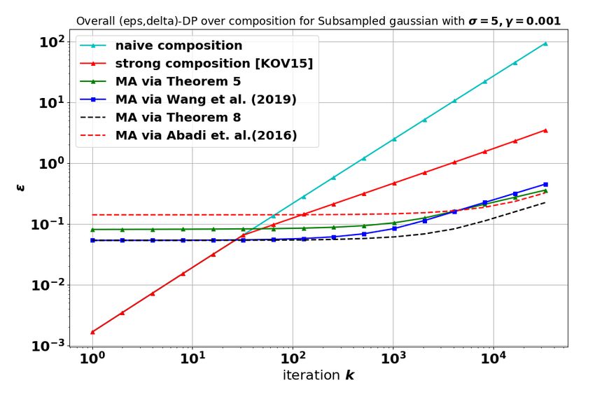
(a) Gaussian mechanism (σ = 5) (b) Laplace mechanism (b = 2) (c) Randomized response (p = 0.6)
(d) Gaussian mechanism (σ = 1) (e) Laplace mechanism (b = 0.5) (f) Randomized response (p = 0.9)
Figure 4. Illustration of the use of our bounds in moments accountant. We plot the the privacy loss ϵ for δ = 1e − 8 (using (2)) after k
rounds of composition. The x-axis is the number of composition k,and the y-axis is the privacy loss after k’s composition. The green
curve is based on general upper bound for all parametrized random mechanism obtained through Theorem 5. Short hand MA refer to
“moment accountant”. The upper three figures are in high privacy regime with parameter σ = 5, b = 2, p = 0.6, the lower three are in
low privacy regime with σ = 1, b = 0.5, p = 0.9.
perform as well as the tight bound when k is large (thanks Future work includes making use of the exact subsampled
to the tightness for small α). RDP bounds to tighten the existing results that made use
of subsampled-mechanisms, coming up with more general
5. Conclusion recipe to automatically check the nonnegativity condition
on the odd-order Pearson-Vajda χα -Divergences and de-
In this paper, we study the problem of privacy- sign differentially private learning algorithms with more
amplification by poisson subsampling, which involves complex and hetereogenous building blocks.
"add/remove" scheme instead of replacement strategy.
Specifically, we derive a tight upper bound for M ◦ Acknowledgements
PoissonSample for any mechanism satisfying that their odd
order Pearson-Vajda χα -Divergences are nonnegative. We YZ and YW were supported by a start-up grant of UCSB
showed that Gaussian mechanism and Laplace mechanism Computer Science Department and a Machine Learning Re-
have this property, as a result, finding the exact analytical search Award from Amazon Web Services. The authors
expression for the Poisson subsampled Gaussian mecha- thank Borja Balle, Shiva Kasiviswanathan, Alex Smola,
nism that has seen significant application in differentially Mu Li and Kunal Talwar for helpful discussions.
private deep learning. Our results imply that we can com-
pletely avoid numerical integration in moments accounts References
and track the entire range of α without paying unbounded
memory. In addition, we propose an efficiently τ -term ap- Abadi, M., Chu, A., Goodfellow, I., McMahan, H. B.,
proximation scheme which only calculates the first and last Mironov, I., Talwar, K., and Zhang, L. Deep learning
τ terms in the Binomial expansion when evaluating the with differential privacy. In ACM SIGSAC Conference
RDP of subsampled mechanisms. This greatly simplifies on Computer and Communications Security (CCS-16),
the computation for computing ϵ given δ as is used in the pp. 308–318. ACM, 2016.
moments accountant. The experiment result of τ -term ap-
proximate part reveals that approximate bound matches up
Balle, B. and Wang, Y.-X. Improving gaussian mechanism
the lower bound quickly even for a relative small τ .
for differential privacy: Analytical calibration and op-Poission Subsampled RDP
timal denoising. International Conference in Machine Li, N., Qardaji, W., and Su, D. On sampling, anonymiza-
Learning (ICML), 2018. tion, and differential privacy or, k-anonymization meets
differential privacy. In The 7th ACM Symposium on In-
Balle, B., Barthe, G., and Gaboardi, M. Privacy amplifi- formation, Computer and Communications Security, pp.
cation by subsampling: Tight analyses via couplings and 32–33. ACM, 2012.
divergences. In Advances in Neural Information Process-
ing Systems (NIPS-18), 2018. McMahan, H. B., Ramage, D., Talwar, K., and Zhang, L.
Learning differentially private recurrent language mod-
Bassily, R., Smith, A., and Thakurta, A. Private empirical els. In International Conference on Learning Represen-
risk minimization: Efficient algorithms and tight error tations (ICLR-18), 2018.
bounds. In Foundations of Computer Science (FOCS-
14), pp. 464–473. IEEE, 2014. Mironov, I. Rényi differential privacy. In Computer Secu-
rity Foundations Symposium (CSF), 2017 IEEE 30th, pp.
Beimel, A., Nissim, K., and Stemmer, U. Characterizing 263–275. IEEE, 2017.
the sample complexity of private learners. In Conference
on Innovations in Theoretical Computer Science (ITCS- Nielsen, F. and Nock, R. On the chi square and higher-order
13), pp. 97–110. ACM, 2013. chi distances for approximating f-divergences. IEEE Sig-
nal Processing Letters, 21(1):10–13, 2014.
Bun, M. and Steinke, T. Concentrated differential privacy:
Simplifications, extensions, and lower bounds. In The- Papernot, N., Song, S., Mironov, I., Raghunathan, A., Tal-
ory of Cryptography Conference, pp. 635–658. Springer, war, K., and Úlfar Erlingsson. Scalable private learning
2016. with pate. In International Conference on Learning Rep-
resentations (ICLR-18), 2018.
Bun, M., Nissim, K., Stemmer, U., and Vadhan, S. Differ-
entially private release and learning of threshold func- Park, M., Foulds, J., Chaudhuri, K., and Welling, M. Vari-
tions. In Foundations of Computer Science (FOCS), ational bayes in private settings (vips). arXiv preprint
2015 IEEE 56th Annual Symposium on, pp. 634–649. arXiv:1611.00340, 2016.
IEEE, 2015.
Särndal, C.-E., Swensson, B., and Wretman, J. Model as-
Bun, M., Dwork, C., Rothblum, G. N., and Steinke, T. sisted survey sampling. Springer Science & Business
Composable and versatile privacy via truncated cdp. In Media, 2003.
Proceedings of the 50th Annual ACM SIGACT Sympo-
Song, S., Chaudhuri, K., and Sarwate, A. D. Stochastic
sium on Theory of Computing, pp. 74–86. ACM, 2018.
gradient descent with differentially private updates. In
Dwork, C. and Rothblum, G. N. Concentrated differential Conference on Signal and Information Processing, 2013.
privacy. arXiv preprint arXiv:1603.01887, 2016.
Vajda, I. χα -divergence and generalized fisher information.
Dwork, C., McSherry, F., Nissim, K., and Smith, A. Cal- In Prague Conference on Information Theory, Statisti-
ibrating noise to sensitivity in private data analysis. In cal Decision Functions and Random Processes, pp. 223.
Theory of cryptography, pp. 265–284. Springer, 2006. Academia, 1973.
Foulds, J., Geumlek, J., Welling, M., and Chaudhuri, K. On Wang, Y.-X., Fienberg, S., and Smola, A. Privacy for
the theory and practice of privacy-preserving bayesian free: Posterior sampling and stochastic gradient monte
data analysis. In Conference on Uncertainty in Artificial carlo. In International Conference on Machine Learning
Intelligence (UAI-16), pp. 192–201. AUAI Press, 2016. (ICML-15), pp. 2493–2502, 2015.
Geumlek, J., Song, S., and Chaudhuri, K. Renyi differential Wang, Y.-X., Lei, J., and Fienberg, S. E. Learning with
privacy mechanisms for posterior sampling. In Advances differential privacy: Stability, learnability and the suffi-
in Neural Information Processing Systems (NIPS-17), pp. ciency and necessity of erm principle. Journal of Ma-
5295–5304, 2017. chine Learning Research, 17(183):1–40, 2016.
Kairouz, P., Oh, S., and Viswanath, P. The composition Wang, Y.-X., Balle, B., and Kasiviswanathan, S. Subsam-
theorem for differential privacy. In International Confer- pled rényi differential privacy and analytical moments
ence on Machine Learning (ICML-15), 2015. accountant. In International Conference on Artificial In-
telligence and Statistics (AISTATS-19), 2019.
Kasiviswanathan, S. P., Lee, H. K., Nissim, K., Raskhod-
nikova, S., and Smith, A. What can we learn privately?
SIAM Journal on Computing, 40(3):793–826, 2011.You can also read