Practical Deep Stereo (PDS): Toward applications-friendly deep stereo matching.
←
→
Page content transcription
If your browser does not render page correctly, please read the page content below
Practical Deep Stereo (PDS): Toward
                                                   applications-friendly deep stereo matching.

                                                        Stepan Tulyakov                                  Anton Ivanov
                                                   Space Engineering Center at                     Space Engineering Center at
                                            École Polytechnique Fédérale de Lausanne        École Polytechnique Fédérale de Lausanne
                                                  stepan.tulyakov@epfl.ch                           anton.ivanov@epfl.ch
arXiv:1806.01677v1 [cs.CV] 5 Jun 2018

                                                                                  Francois Fleuret
                                                                      École Polytechnique Fédérale de Lausanne
                                                                             and Idiap Research Institute
                                                                          francois.fleuret@idiap.ch

                                                                                    Abstract

                                                 End-to-end deep-learning networks recently demonstrated extremely good perfor-
                                                 mance for stereo matching. However, existing networks are difficult to use for
                                                 practical applications since (1) they are memory-hungry and unable to process even
                                                 modest-size images, (2) they have to be trained for a given disparity range.
                                                 The Practical Deep Stereo (PDS) network that we propose addresses both issues:
                                                 First, its architecture relies on novel bottleneck modules that drastically reduce
                                                 the memory footprint in inference, and additional design choices allow to handle
                                                 greater image size during training. This results in a model that leverages large
                                                 image context to resolve matching ambiguities. Second, a novel sub-pixel cross-
                                                 entropy loss combined with a MAP estimator make this network less sensitive to
                                                 ambiguous matches, and applicable to any disparity range without re-training.
                                                 We compare PDS to state-of-the-art methods published over the recent months, and
                                                 demonstrate its superior performance on FlyingThings3D and KITTI sets.

                                        1   Introduction

                                        Stereo matching consists in matching every point from an image taken from one viewpoint to
                                        its physically corresponding one in the image taken from another viewpoint. The problem has
                                        applications in robotics Menze and Geiger [2015], medical imaging Nam et al. [2012], remote
                                        sensing Shean et al. [2016], virtual reality and 3D graphics and computational photography Wang
                                        et al. [2016], Barron et al. [2015].
                                        Recent developments in the field have been focused on stereo for hard / uncontrolled environ-
                                        ments (wide-baseline, low-lighting, complex lighting, blurry, foggy, non-lambertian) Verleysen and
                                        De Vleeschouwer [2016], Jeon et al. [2016], Chen et al. [2015], Galun et al. [2015], QUeau et al.
                                        [2017], usage of high-order priors and cues Hadfield and Bowden [2015], Güney and Geiger [2015],
                                        Kim and Kim [2016], Li et al. [2016], Ulusoy et al. [2017], and data-driven, and in particular, deep
                                        neural network based, methods Park and Yoon [2015], Chen et al. [2015], Žbontar and LeCun [2015],
                                        Zbontar and LeCun [2016], Luo et al. [2016], Tulyakov et al. [2017], Seki and Pollefeys [2017],
                                        Knöbelreiter et al. [2017], Shaked and Wolf [2017], Gidaris and Komodakis [2017], Kendall et al.
                                        [2017], Mayer et al. [2016], Pang et al. [2017], Chang and Chen [2018], Liang et al. [2018], Zhong
                                        et al. [2017]. This work improves on this latter line of research.

                                        Preprint. Work in progress.
Table 1: Number of parameters, inference memory footprint, 3-pixels-error (3PE) and mean-absolute-
error on FlyingThings3D (960 × 540 with 192 disparities). DispNetCorr1D Mayer et al. [2016],
CRL Pang et al. [2017], iResNet-i2 Liang et al. [2018] and LRCR Jie et al. [2018] predict disparities
as classes and are consequently over-parameterized. GC Kendall et al. [2017] omits an explicit
correlation step, which results in a large memory usage during inference. Our PDS has a small
number of parameters and memory footprint, the smallest 3PE and second smallest MAE, and it is
the only method able to handle different disparity ranges without re-training. Note that we follow
the protocol of PSM Chang and Chen [2018], and calculate the errors only for ground truth pixel
with disparity < 192. Inference memory footprints are our theoretical estimates based on network
structures and do not include memory required for storing networks’ parameters (real memory
footprint will depend on implementation). Error rates and numbers of parameters are taken from the
respective publications.
Params Memory 3EP MAE Modify.
Method
[M] [GB] [%] [px] Disp.
PDS (proposed) 2.2 0.4 3.38 1.12 3
PSM Chang and Chen [2018] 5.2 0.6 n/a 1.09 7
CRL Pang et al. [2017] 78 0.2 6.20 1.32 7
iResNet-i2 Liang et al. [2018] 43 0.2 4.57 1.40 7
DispNetCorr1D Mayer et al. [2016] 42 0.1 n/a 1.68 7
LRCR Jie et al. [2018] 30 9.0 8.67 2.02 7
GC Kendall et al. [2017] 3.5 4.5 9.34 2.02 7
The first successes of neural networks for stereo matching were achieved by substitution of hand-
crafted similarity measures with deep metrics Chen et al. [2015], Žbontar and LeCun [2015], Zbontar
and LeCun [2016], Luo et al. [2016], Tulyakov et al. [2017] inside a legacy stereo pipeline for the post-
processing (often Mei et al. [2011]). Besides deep metrics, neural networks were also used in other
subtasks such as predicting a smoothness penalty in a CRF model from a local intensity pattern Seki
and Pollefeys [2017], Knöbelreiter et al. [2017]. In Shaked and Wolf [2017] a “global disparity”
network smooth the matching cost volume and predicts matching confidences, and in Gidaris and
Komodakis [2017] a network detects and fixes incorrect disparities.
End-to-end deep stereo. Recent works attempt at solving stereo matching using neural network
trained end-to-end without post-processing Dosovitskiy et al. [2015], Mayer et al. [2016], Kendall
et al. [2017], Zhong et al. [2017], Pang et al. [2017], Jie et al. [2018], Liang et al. [2018], Chang
and Chen [2018]. Such a network is typically a pipeline composed of embedding, matching,
regularization and refinement modules:
The embedding module produces image descriptors for left and right images, and the (non-
parametric) matching module performs an explicit correlation between shifted descriptors to compute
a cost volume for every disparity Dosovitskiy et al. [2015], Mayer et al. [2016], Pang et al. [2017], Jie
et al. [2018], Liang et al. [2018]. This matching module may be absent, and concatenated left-right
descriptors directly fed to the regularization module Kendall et al. [2017], Chang and Chen [2018],
Zhong et al. [2017]. This strategy uses more context, but the deep network implementing such
a module has a larger memory footprint as shown in Table 1. In this work we reduce memory
use without sacrificing accuracy by introducing a matching module that compresses concatenated
left-right image descriptors into compact matching signatures.
The regularization module takes the cost volume, or the concatenation of descriptors, regularizes
it, and outputs either disparities Mayer et al. [2016], Dosovitskiy et al. [2015], Pang et al. [2017],
Liang et al. [2018] or a distribution over disparities Kendall et al. [2017], Zhong et al. [2017], Jie
et al. [2018], Chang and Chen [2018]. In the latter case, sub-pixel disparities can be computed as
a weighted average with SoftArgmin, which is sensitive to erroneous minor modes in the inferred
distribution.
This regularization module is usually implemented as a hourglass deep network with shortcut
connections between the contracting and the expanding parts Mayer et al. [2016], Dosovitskiy et al.
[2015], Pang et al. [2017], Kendall et al. [2017], Zhong et al. [2017], Chang and Chen [2018],
Liang et al. [2018]. It composed of 2D convolutions and not treat all disparities symmetrically in
2some models Mayer et al. [2016], Dosovitskiy et al. [2015], Pang et al. [2017], Liang et al. [2018],
which makes the network over-parametrized and prohibits the change of the disparity range without
modification of its structure and re-training. Or it can use 3D convolutions that treat all disparities
symmetrically Kendall et al. [2017], Zhong et al. [2017], Jie et al. [2018], Chang and Chen [2018]. As
a consequence these networks have less parameters, but their disparity range is still is non-adjustable
without re-training due to SoftArgmin as we show in § 3.3. In this work, we propose to use a novel
sup-pixel MAP approximation for inference which computes a weighted mean around the disparity
with maximum posterior probability. It is more robust to erroneous modes in the distribution and
allows to modify the disparity range without re-training.
Finally, some methods Pang et al. [2017], Liang et al. [2018], Jie et al. [2018] also have a refinement
module, that refines the initial low-resolution disparity relying on attention map, computed as left-
right warping error. The training of end-to-end networks is usually performed in fully supervised
manner (except of Zhong et al. [2017]).
All described methods Dosovitskiy et al. [2015], Mayer et al. [2016], Kendall et al. [2017], Zhong
et al. [2017], Pang et al. [2017], Jie et al. [2018], Liang et al. [2018], Chang and Chen [2018] use
modest-size image patches during training. In this work, we show that training on a full-size images
boosts networks ability to utilize large context and improves its accuracy. Also, the methods, even
the ones producing disparity distribution, rely on L1 loss, since it allows to train network to produce
sub-pixel disparities. We, instead propose to use more “natural” sub-pixel cross-entropy loss that
ensures faster converges and better accuracy.
Our contributions can be summarize as follows:
1. We decrease the memory footprint by introducing a novel bottleneck matching module. It
compresses the concatenated left-right image descriptors into compact matching signatures, which
are then concatenated and fed to the hourglass network we use as regularization module, instead
of the concatenated descriptors themselves as in Kendall et al. [2017], Chang and Chen [2018].
Reduced memory footprint allows to process larger images and to train on a full-size images, that
boosts networks ability to utilize large context.
2. Instead of computing the posterior mean of the disparity and training with a vanilla L1
penalty Chang and Chen [2018], Jie et al. [2018], Zhong et al. [2017], Kendall et al. [2017]
we propose for inference a sub-pixel MAP approximation that computes a weighted mean around
the disparity with maximum posterior probability, which is robust to erroneous modes in the
disparity distribution and allows to modify the disparity range without re-training. For training we
similarly introduce a sub-pixel criterion by combining the standard cross-entropy with a kernel
interpolation, which provides faster convergence rates and higher accuracy.
In the experimental section, we validate our contributions. In § 3.2 we show how the reduced
memory footprint allows to train on full-size images and to leverage large image contexts to improve
performance. In § 3.3 we demonstrate that, thanks to the proposed sub-pixel MAP and cross-entropy,
we are able to modify the disparity range without re-training, and to improve the matching accuracy.
Than, in § 3.4 we compare our method to state-of-the-art baselines and show that it has smallest
3-pixels error (3PE) and second smallest mean absolute error (MAE) on the FlyingThings3D set and
ranked third and fourth on KITTI’15 and KITTI’12 sets respectively.
2 Method
2.1 Network structure
Our network takes as input the left and right color images {xL , xR } of size W × H and produces a
“cost tensor” C = N et(xL , xR | Θ, D) of size D 2 × W × H, where Θ are the model’s parameters,
an D ∈ N is the maximum disparity.
The computed cost tensor is such that Ck,i,j is the cost of matching the pixel xL
i,j in the left image to
R
the pixel xi−2k,j in the right image, which is equivalent to assigning the disparity di,j = 2k to the
left image pixel.
This cost tensor C can then be converted into an a posterior probability tensor as
P d | xL , xR = softmax (−C) .
332 x W x H 32 x W/4 x H/4 Inference
Right Right 8
image descriptor WxH
Compact
Sub-pix. MAP
8 x D/4
matching Disparity
signatures
estimator
Cost
volume
Regularization
H/4
D / 4 pairs
Match network
(3D conv.) H Training
W/4 D/2 WxH
W Sub-pix. Ground
Cross Entropy truth
32 x W x H
Left
image Left
descriptor
32 x W/4 x H/4
Figure 1: Network structure and processing flow during training and inference. Input / output
quantities are outlined with thin lines, while processing modules are drawn with thick ones. Following
the vocabulary introduced in § 1, the yellow shapes are embedding modules, the red rectangle the
matching module and the blue shape the the regularization module. The matching module is a
contribution of our work, as in previous methods Kendall et al. [2017], Chang and Chen [2018] left
and shifted right descriptors are directly fed to the regularization module (hourglass network). Note
that the concatenated compact matching signature tensor is a 4D tensor represented here as 3D by
combining the feature indexes and disparities along the vertical axis.
The overall structure of the network and processing flow during training and inference are shown in
Figure 1, and we can summarize for clarity the input/output to and from each of the modules:
• The embedding module takes as input a color image 3×W ×H, and computes an image descriptor
32 × W H
4 × 4.
• The matching module takes as input, for each disparity d, a left and a (shifted) right image
descriptor both 32 × W H W H
4 × 4 , and computes a compact matching signature 8 × 4 × 4 . This
module is unique to our network and described in details in § 2.2.
• The regularization module is a hourglass 3D convolution neural network with shortcut connections
between the contracting and the expanding parts. It takes a tensor composed of concatenated
compact matching signatures for all disparities of size 8 × D W H
4 × 4 × 4 , and computes a matching
D
cost tensor C of size 2 × W × H.
Additional information such as convolution filter size or channel numbers is provided in the Supple-
mentary materials.
According to the taxonomy in Scharstein and Szeliski [2001] all traditional stereo matching methods
consist of (1) matching cost computation, (2) cost aggregation, (3) optimization, and (4) disparity
refinement steps. In the proposed network, the embedding and the matching modules are roughly
responsible for the step (1) and the regularization module for the steps (2-4).
Besides the matching module, there are several other design choices that reduce test and training
memory footprint of our network. In contrast to Kendall et al. [2017] we use aggressive four-
times sub-sampling in the embedding module, and the hourglass DNN we use for regularization
module produces probabilities only for even disparities. Also, after each convolution and transposed
convolution in our network we place Instance Normalization (IN) Ulyanov et al. [2016] instead of
Batch Normalization (BN) as show in the Supplementary materials, since we use individual full-size
images during training.
2.2 Matching module
The core of state-of-the-art methods Kendall et al. [2017], Zhong et al. [2017], Jie et al. [2018], Chang
and Chen [2018] is the 3D convolutions Hourglass network used as regularization module, that
takes as input a tensor composed of concatenated left-right image descriptor for all possible disparity
values. The size of this tensor makes such networks have a huge memory footprint during inference.
We decrease the memory usage by implementing a novel matching with a DNN with a “bottle-
neck” architecture. This module compresses the concatenated left-right image descriptors into a
compact matching signature for each disparity, and the results is then concatenated and fed to the
Hourglass module. This contrasts with existing methods, which directly feed the concatenated
descriptors Kendall et al. [2017], Zhong et al. [2017], Jie et al. [2018], Chang and Chen [2018].
4Target distribution
Sub-pixel MAP SoftArgmin Sub-pixel MAP SoftArgmin
estimation estimation estimation estimation
Ground Truth
(a) (b)
Figure 3: Target distri-
Figure 2: Comparison the proposed Sub-pixel MAP with the standard bution of sub-pixel cross-
SoftArgmin: (a) in presence of a multi-modal distribution SoftArgmin entropy is a discretized
blends all the modes and produces an incorrect disparity estimate. (b) Laplace distribution cen-
when the disparity range is extended (blue area), SoftArgmin estimate tered at sub-pixel ground-
may degrade due to additional modes. truth disparity.
This module is inspired by CRL Pang et al. [2017] and DispNetCorr1D Pang et al. [2017], Mayer
et al. [2016] which control the memory footprint (as shown in Table 1 by feeding correlation results
instead of concatenated embeddings to the Hourglass network and by Zagoruyko and Komodakis
[2015] that show superior performance of joint left-right image embedding. We also borrowed some
ideas from the bottleneck module in ResNet He et al. [2016], since it also encourages compressed
intermediate representations.
2.3 Sub-pixel MAP
In state-of-the-art methods, a network produces an posterior disparity distribution and then use a
SoftArgmin module Kendall et al. [2017], Zhong et al. [2017], Jie et al. [2018], Chang and Chen
[2018], introduced in Kendall et al. [2017], to compute the predicted sub-pixel disparity as an
expectation of this distribution:
X
dˆ = d · P d = d | xL , xR .
d
This SoftArgmin approximates a sub-pixel maximum a posteriori (MAP) solution when the distri-
bution is unimodal and symmetric. However, as illustrated in Figure 2, this strategy suffers from
two key weaknesses: First, when these assumptions are not fulfilled, for instance if the posterior is
multi-modal, this averaging blends the modes and produces a disparity estimate far from all of them.
Second, if we want to apply the model to a greater disparity range without re-training, the estimate
may degrade even more due to additional modes.
The authors of Kendall et al. [2017] argue that when the network is trained with the SoftArgmin, it
adapts to it during learning by rescaling its output values to make the distribution unimodal. However,
the network learns rescaling only for disparity range used during training. If we decide to change the
disparity range during the test, we will have to re-train the network.
To address both of these drawbacks, we propose to use for inference a sub-pixel MAP approximation
that computes a weighted mean around the disparity with maximum posterior probability as
X
d˜ = d · P d = d | xL , xR , where dˆ = arg max P d = d | xL , xR ,
(1)
1≤d≤D
d:|d−d
ˆ |≤δ
with δ a meta-parameter (in our experiments we choose δ = 4 based on small scale grid search
experiment on the validation set). The approximation works under assumption that the distribution is
symmetric in a vicinity of a major mode.
In contrast to the SoftArgmin, the proposed sup-pixel MAP is used only for inference. During training
we use the posterior disparity distribution and the sub-pixel cross-entropy loss discussed in the next
section.
2.4 Sub-pixel cross-entropy
Many methods use the L1 loss Chang and Chen [2018], Jie et al. [2018], Zhong et al. [2017], Kendall
et al. [2017], even though the “natural” choice for the network that produces the posterior distribution
is a cross-entropy. The L1 loss is often selected because it empirically Kendall et al. [2017] performs
5better than cross-entropy, and because when it is combined with SoftArgmin, it allows to train a
network with sub-pixel ground truth.
In this work, we propose a novel sub-pixel cross-entropy that provides faster convergence and better
accuracy. The target distribution of our cross-entropy loss is a discretized Laplace distribution
centered at the ground-truth disparity dgt , shown in Figure 3 and computed as
|d − dgt | |i − dgt |
1 X
Qgt (d) = exp − , where N = exp − ,
N b i
b
where b is a diversity of the Laplace distribution (in our experiments we set b = 2, reasoning that the
distribution should reasonably cover at least several discrete disparities). With this target distribution
we compute cross-entropy as usual
X
Qgt (d) · log P d = d | xL , xR , Θ .
L(Θ) = (2)
d
The proposed sub-pixel cross-entropy is different from soft cross entropy Luo et al. [2016], since
in our case probability in each discrete location of the target distribution is a smooth function of a
distance to the sub-pixel ground-truth. This allows to train the network to produce a distribution from
which we can compute sub-pixel disparities using our sub-pixel MAP.
3 Experiments
Our experiments are done with the PyTorch framework PyTorch. We initialize weights and biases of
the network using default PyTorch initialization and train the network as shown in Table 2. During the
training we normalize training patches to zero mean and unit variance. The optimization is performed
with the RMSprop method with standard settings.
Table 2: Summary of training settings for every dataset.
FlyingThings3D KITTI
Mode from scratch fine-tune
Lr. schedule 0.01 for 120k, half every 20k 0.005 for 50k, half every 20k
Iter. # 160k 100k
Tr. image size 960 × 540 full-size 1164 × 330
Max disparity 255 255
Augmentation not used mixUp Zhang et al. [2018], anisotropic zoom, random crop
We guarantee reproducibility of all experiments in this section by using only available data-sets, and
making our code available online under open-source license after publication.
3.1 Datasets and performance measures
We used three data-sets for our experiments: KITTI’12 Geiger et al. [2012] and KITTI’15 Menze
and Geiger [2015], that we combined into a KITTI set, and FlyingThings3D Mayer et al. [2016]
summarized in Table 3. KITTI’12, KITTI’15 sets have online scoreboards KITTY.
The FlyingThings3D set suffers from two problems: (1) as noticed in Pang et al. [2017], Zhang et al.
[2018], some images have very large (up to 103 ) or negative disparities; (2) some images are rendered
with black dots artifacts. For the training we use only images without artifacts and with disparities
∈ [0, 255].
We noticed that this is dealt with in some previous publications by processing the test set using the
ground truth for benchmarking, without mentioning it. Such pre-processing may consist of ignoring
pixels with disparity > 192 Chang and Chen [2018], or discarding images with more than 25% of
pixels with disparity > 300 Pang et al. [2017], Liang et al. [2018]. Although this is not commendable,
for the sake of comparison we followed the same protocol as Chang and Chen [2018] which is the
method the closest to ours in term of performance. In all other experiments we use the unaltered test
set.
6We make validation sets by withholding 500 images from the FlyingThings3D training set, and 58
from the KITTI training set, respectively.
Table 3: Datasets used for experiments. During benchmarking, we follow previous works and use
maximum disparity, that is different from absolute maximum for the datasets, provided between
parentheses.
Dataset Test # Train # Size Max disp. Ground truth Web score
KITTI 395 395 1226 × 370 192 (230) sparse, ≤ 3 px. 3
FlyingThings3D 4370 25756 960 × 540 192 (6773) dense , unknown 7
We measure the performance of the network using two standard measures: (1) 3-pixel-error (3PE),
which is the percentage of pixels for which the predicted disparity is off by more than 3 pixels, and
(2) mean-absolute-error (MAE), the average difference of the predicted disparity and the ground truth.
Note, that 3PE and MAE are complimentary, since 3PE characterize error robust to outliers, while
MAE accounts for sub-pixel error.
3.2 Training on full-size images
In this section we show the effectiveness of training on full-size images. For that we train our network
till convergence on FlyingThings3D dataset with the L1 loss and SoftArgmin twice, the first time
we use 512 × 256 training patches randomly cropped from the training images as in Kendall et al.
[2017], Chang and Chen [2018], and the second time we used full-size 960 × 540 training images.
Note, that the latter is possible thanks to the small memory footprint of our network.
As seen in Table 4, the network trained on small patches, performs better on larger than on smaller
test images. This suggests, that even the network that has not seen full-size images during training
can utilize a larger context. As expected, the network trained on full-size images makes better use of
the said context, and performs significantly better.
3.3 Sub-pixel MAP and cross-entropy
Sub-pix CrossEntropy
8 L1
7
validation set 3PE
6
5
4
3
2.5 5.0 7.5 10.0 12.5 15.0 17.5 20.0
epoch
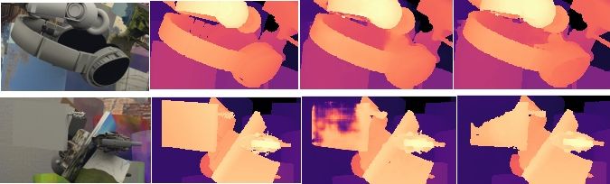
Figure 4: Example of disparity estimation errors with the Sof- Figure 5: Comparison of the
tArgmin and sup-pixel MAP on FlyingThings3d set. The first convergence speed on FlyingTh-
column shows image, the second – ground truth disparity, the third ings3d set with sub-pixel cross
– SoftArgmin estimate and the fourth sub-pixel MAP estimate. Note entropy and L1 loss. Note that
that SoftArgmin estimate, though completely wrong, is closer to with the proposed sub-pixel cross-
the ground truth than sub-pixel MAP estimate. This can explain entropy loss (blue) network con-
larger MAE of the sub-pixel MAP estimate. verges faster.
Table 4: Error of the proposed PDS network on FlyingThings3d set as a function of training patch
size. The network trained on full-size images (highlighted), outperforms the network trained on small
image patches. Note, that in this experiment we used SoftArgmin with L1 loss during training.
Train size Test size 3PE, [%] MAE, [px]
512 × 256 512 × 256 8.63 4.18
512 × 256 960 × 540 5.28 3.55
960 × 540 960 × 540 4.50 3.40
7In this section, we firstly show the advantages of the sub-pixel MAP over the SoftArgmin. We train
the our PDS network till convergence on FlyingThings3D with SoftArgmin, L1 loss and full-size
training images and then test it twice: the first time with SoftArgmin for inference, and the second
time with our sub-pixel MAP for inference instead.
As shown in Table 5, the substitution leads to the reduction of the 3PE and slight increase of the
MAE. The latter probably happens because in the erroneous area SoftArgmin estimate are completely
wrong, but nevertheless closer to the ground truth since it blends all distribution modes, as shown in
Figure 4.
Table 5: Performance of the sub-pixel MAP estimator and cross-entropy loss on FlyingThings3d set.
Note, that: (1) if we substitute SoftArgmin with sub-pixel MAP during the test we get lower 3PE and
similar MAE; (2) if we increase disparity range twice MAE and 3PE of the network with sub-pixel
MAP almost does not change, while errors of the network with SoftArgmin increase; (3) if we train
network with with sub-pixel cross entropy it has much lower 3PE and only slightly worse MAE.
Loss Estimator 3PE, [%] MAE, [px]
Standard disparity range ∈ [0, 255]
L1 + SoftArgmin SoftArgmin 4.50 3.40
L1 + SoftArgmin Sub-pixel MAP 4.22 3.42
Sub-pixel cross-entropy. Sub-pixel MAP 3.80 3.63
Increased disparity range ∈ [0, 511]
L1 + SoftArgmin SoftArgmin 5.20 3.81
L1 + SoftArgmin Sub-pixel MAP 4.27 3.53
When we test the same network with the disparity range increased from 255 to 511 pixels the
performance of the network with the SoftArgmin plummets, while performance of the network with
sub-pixel MAP remains almost the same as shown in Table 5. This shows that with Sub-pixel MAP
we can modify the disparity range of the network on-the-fly, without re-training.
Next, we train the network with the sub-pixel cross-entropy loss and compare it to the network trained
with SoftArgmin and the L1 loss. As show in Table 5, the former network has much smaller 3PE
and only slightly larger MAE. The convergence speed with sub-pixel cross-entropy is also much
faster than with L1 loss as shown in Figure 5. Interestingly, in Kendall et al. [2017] also reports faster
convergence with one-hot cross-entropy than with L1 loss, but contrary to our results, they found that
L1 provided smaller 3PE.
3.4 Benchmarking
In this section we show the effectiveness of our method, compared to the state-of-the-art methods.
For KITTI, we computed disparity maps for the test sets with withheld ground truth, and uploaded
the results to the evaluation web site. For the FlyingThings3D set we evaluated performance on the
test set ourselves, following the protocol of Chang and Chen [2018] as explained in § 3.1.
FlyingThings3D set benchmarking results are shown in Table 1. Notably, the method we propose
has lowest 3PE error and second lowest MAE. Moreover, in contrast to other methods, our method has
small memory footprint, number of parameters, and it allows to change the disparity range without
re-training.
KITTI’12, KITTI’15 benchmarking results are shown in Table 6. The method we propose ranks
third on KITTI’15 set and fourth on KITTI’12 set, taking into account state-of-the-art results published
a few months ago or not officially published yet iResNet-i2 Liang et al. [2018], PSMNet Chang and
Chen [2018] and LRCR Jie et al. [2018] methods.
4 Conclusion
In this work we addressed two issues precluding the use of deep networks for stereo matching in
many practical situations in spite of their excellent accuracy: their large memory footprint, and the
inability to adjust to a different disparity range without complete re-training.
8Table 6: KITTI’15 (top) and KITTI’12 (bottom) snapshots from 15/05/2018 with top-10 methods,
including published in a recent months on not officially published yet: iResNet-i2 Liang et al. [2018],
PSMNet Chang and Chen [2018] and LRCR Jie et al. [2018]. Our method (highlighted) is 3rd in
KITTI’15 and 4th in KITTI’12 leader boards.
# dd/mm/yy Method 3PE (all pixels), [%] Time, [s]
1 30/12/17 PSMNet Chang and Chen [2018] 2.16 0.4
2 18/03/18 iResNet-i2 Liang et al. [2018] 2.44 0.12
3 15/05/18 PSN (proposed) 2.58 0.5
4 24/03/17 CRL Pang et al. [2017] 2.67 0.47
5 27/01/17 GC-NET Kendall et al. [2017] 2.87 0.9
6 15/11/17 LRCR Jie et al. [2018] 3.03 49
7 15/11/16 DRR Gidaris and Komodakis [2017] 3.16 0.4
8 08/11/17 SsSMnet Zhong et al. [2017] 3.40 0.8
9 15/12/16 L-ResMatch Shaked and Wolf [2017] 3.42 48
10 26/10/15 Displets v2 Güney and Geiger [2015] 3.43 265
# dd/mm/yy Method 3PE (non-occluded), [%] Time, [s]
1 31/12/17 PSMNet Chang and Chen [2018] 1.49 0.4
2 23/11/17 iResNet-i2 Liang et al. [2018] 1.71 0.12
3 27/01/17 GC-NET Kendall et al. [2017] 1.77 0.9
4 15/05/18 PSN (proposed) 1.92 0.5
5 15/12/16 L-ResMatch Shaked and Wolf [2017] 2.27 48
6 11/09/16 CNNF+SGM Zhang and Wah [2018] 2.28 71
7 15/12/16 SGM-NET Seki and Pollefeys [2017] 2.29 67
8 08/11/17 SsSMnet Zhong et al. [2017] 2.30 0.8
9 27/04/16 PBCP Seki and Pollefeys [2016] 2.36 68
10 26/10/15 Displets v2 Güney and Geiger [2015] 2.37 265
We showed that by carefully revising conventionally used networks architecture to control the memory
footprint and adapt analytically the network to the disparity range, and by using a new loss and
estimator to cope with multi-modal posterior and sub-pixel accuracy, it is possible to resolve these
practical issues and reach state-of-the-art performance.
References
Jonathan T Barron, Andrew Adams, YiChang Shih, and Carlos Hernández. Fast bilateral-space stereo
for synthetic defocus. In CVPR, 2015.
Jia-Ren Chang and Yong-Sheng Chen. Pyramid stereo matching network. CoRR, 2018.
Zhuoyuan Chen, Xun Sun, and Liang Wang. A Deep Visual Correspondence Embedding Model for
Stereo Matching Costs. ICCV, 2015.
Alexey Dosovitskiy, Philipp Fischer, Eddy Ilg, Philip Hausser, Caner Hazirbas, Vladimir Golkov,
Patrick van der Smagt, Daniel Cremers, and Thomas Brox. Flownet: Learning optical flow with
convolutional networks. In CVPR, 2015.
Meirav Galun, Tal Amir, Tal Hassner, Ronen Basri, and Yaron Lipman. Wide baseline stereo matching
with convex bounded distortion constraints. In ICCV, 2015.
Andreas Geiger, Philip Lenz, and Raquel Urtasun. Are we ready for autonomous driving? the kitti
vision benchmark suite. In CVPR, 2012.
Spyros Gidaris and Nikos Komodakis. Detect, replace, refine: Deep structured prediction for pixel
wise labeling. CVPR, 2017.
Fatma Güney and Andreas Geiger. Displets: Resolving Stereo Ambiguities using Object Knowledge.
CVPR, 2015.
9Simon Hadfield and Richard Bowden. Exploiting high level scene cues in stereo reconstruction. In
ICCV, 2015.
Kaiming He, Xiangyu Zhang, Shaoqing Ren, and Jian Sun. Deep residual learning for image
recognition. In CVPR, 2016.
Hae-Gon Jeon, Joon-Young Lee, Sunghoon Im, Hyowon Ha, and In So Kweon. Stereo matching
with color and monochrome cameras in low-light conditions. In CVPR, 2016.
Zequn Jie, Pengfei Wang, Yonggen Ling, Bo Zhao, Yunchao Wei, Jiashi Feng, and Wei Liu. Left-right
comparative recurrent model for stereo matching. In CVPR, 2018.
Alex Kendall, Hayk Martirosyan, Saumitro Dasgupta, Peter Henry, Ryan Kennedy, Abraham
Bachrach, and Adam Bry. End-to-end learning of geometry and context for deep stereo regression.
ICCV, 2017.
K. R. Kim and C. S. Kim. Adaptive smoothness constraints for efficient stereo matching using texture
and edge information. In ICIP, 2016.
KITTY. Kitti stereo scoreboards. http://www.cvlibs.net/datasets/kitti/ Accessed: 05
May 2018.
Patrick Knöbelreiter, Christian Reinbacher, Alexander Shekhovtsov, and Thomas Pock. End-to-end
training of hybrid cnn-crf models for stereo. CVPR, 2017.
Ang Li, Dapeng Chen, Yuanliu Liu, and Zejian Yuan. Coordinating multiple disparity proposals for
stereo computation. In CVPR, 2016.
Zhengfa Liang, Yiliu Feng, Yulan Guo Hengzhu Liu Wei Chen, and Linbo Qiao Li Zhou Jianfeng
Zhang. Learning for disparity estimation through feature constancy. CoRR, 2018.
Wenjie Luo, Alexander G Schwing, and Raquel Urtasun. Efficient deep learning for stereo matching.
In CVPR, 2016.
Nikolaus Mayer, Eddy Ilg, Philip Hausser, Philipp Fischer, Daniel Cremers, Alexey Dosovitskiy, and
Thomas Brox. A large dataset to train convolutional networks for disparity, optical flow, and scene
flow estimation. In CVPR, 2016.
Xing Mei, Xun Sun, Mingcai Zhou, Shaohui Jiao, Haitao Wang, and Xiaopeng Zhang. On building
an accurate stereo matching system on graphics hardware. In ICCV Workshops, 2011.
Moritz Menze and Andreas Geiger. Object scene flow for autonomous vehicles. In CVPR, 2015.
Kyoung Won Nam, Jeongyun Park, In Young Kim, and Kwang Gi Kim. Application of stereo-imaging
technology to medical field. Healthcare informatics research, 2012.
Jiahao Pang, Wenxiu Sun, JS Ren, Chengxi Yang, and Qiong Yan. Cascade residual learning: A
two-stage convolutional neural network for stereo matching. In ICCVW, 2017.
Min-Gyu Park and Kuk-Jin Yoon. Leveraging stereo matching with learning-based confidence
measures. In CVPR, 2015.
PyTorch. Pytorch web site. http://http://pytorch.org/ Accessed: 05 May 2018.
Yvain QUeau, Tao Wu, François Lauze, Jean-Denis Durou, and Daniel Cremers. A non-convex
variational approach to photometric stereo under inaccurate lighting. In CVPR, 2017.
Daniel Scharstein and Richard Szeliski. A Taxonomy and Evaluation of Dense Two-Frame Stereo
Correspondence Algorithms. IJCV, 2001.
Akihito Seki and Marc Pollefeys. Patch based confidence prediction for dense disparity map. In
BMVC, 2016.
Akihito Seki and Marc Pollefeys. Sgm-nets: Semi-global matching with neural networks. 2017.
10Amit Shaked and Lior Wolf. Improved stereo matching with constant highway networks and reflective
confidence learning. CVPR, 2017.
David E Shean, Oleg Alexandrov, Zachary M Moratto, Benjamin E Smith, Ian R Joughin, Claire
Porter, and Paul Morin. An automated, open-source pipeline for mass production of digital
elevation models (DEMs) from very-high-resolution commercial stereo satellite imagery. {ISPRS},
2016.
S. Tulyakov, A. Ivanov, and F. Fleuret. Weakly supervised learning of deep metrics for stereo
reconstruction. In ICCV, 2017.
Ali Osman Ulusoy, Michael J Black, and Andreas Geiger. Semantic multi-view stereo: Jointly
estimating objects and voxels. In CVPR, 2017.
Dmitry Ulyanov, Andrea Vedaldi, and Victor S. Lempitsky. Instance normalization: The missing
ingredient for fast stylization. CoRR, 2016.
Cedric Verleysen and Christophe De Vleeschouwer. Piecewise-planar 3d approximation from wide-
baseline stereo. In CVPR, 2016.
Ting-Chun Wang, Manohar Srikanth, and Ravi Ramamoorthi. Depth from semi-calibrated stereo and
defocus. In CVPR, 2016.
Sergey Zagoruyko and Nikos Komodakis. Learning to compare image patches via convolutional
neural networks. 2015.
Jure Žbontar and Yann LeCun. Computing the Stereo Matching Cost With a Convolutional Neural
Network. CVPR, 2015.
Jure Zbontar and Yann LeCun. Stereo matching by training a convolutional neural network to
compare image patches. JMLR, 2016.
F. Zhang and B. W. Wah. Fundamental principles on learning new features for effective dense
matching. IEEE Transactions on Image Processing, 27(2):822–836, Feb 2018. ISSN 1057-7149.
doi: 10.1109/TIP.2017.2752370.
Hongyi Zhang, Moustapha Cisse, Yann N. Dauphin, and David Lopez-Paz. mixup: Beyond empirical
risk minimization. In International Conference on Learning Representations, 2018.
Yiran Zhong, Yuchao Dai, and Hongdong Li. Self-supervised learning for stereo matching with
self-improving ability. CoRR, 2017.
11You can also read