Predicting The Invasion Risk of Non-Native Reptiles as Pets in The Middle East
←
→
Page content transcription
If your browser does not render page correctly, please read the page content below
Predicting The Invasion Risk of Non-Native Reptiles as Pets in The Middle
East
Azita Farashi ( farashi@um.ac.ir )
Ferdowsi University of Mashhad
Mohammad Alizadeh-Noughani
Ferdowsi University of Mashhad
Research
Keywords: SDM, Pet, Habitat, Distribution, Potential range.
Posted Date: June 29th, 2021
DOI: https://doi.org/10.21203/rs.3.rs-633913/v1
License: This work is licensed under a Creative Commons Attribution 4.0 International License. Read Full License
Page 1/14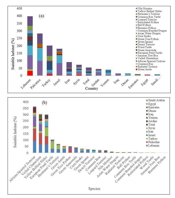
Abstract
Wildlife trade for non-native pets is an important and increasing driver of biodiversity loss and often compromises the standards required for protection.
However, the growing interest in non-native pets has posed the issue of invasive non-native species to wildlife managers and conservationists. Instituting
effective policies regarding non-native species requires a thorough understanding of the potential range of the species in new environments. In this study, we
used an ensemble of ten species distribution models to predict the potential distribution for 23 commonly traded species of reptiles across the Middle East.
We used ten modeling techniques implemented in the Biomod2 package and ensemble forecasts. Final models contained fourteen environmental variables,
including climatic, topographic, and land cover/land use variables. Our results indicate that all Middle Eastern countries included suitable habitats for at least
six species, except Qatar, Kuwait and Bahrain for which the models did not predict any suitable habitats. Our study showed that Lebanon, Palestine, Turkey,
and Israel face the highest risk of biological invasion by the species on the whole. Also, the results showed that Centrochelys sulcata, Chamaeleo calyptratus,
and Trachemys scripta posed the highest risk of spreading in this area. Information on which species pose a greater danger as invaders and the possible
impacts of their introduction will be a valuable contribution to the development of conservation plans and policies.

Introduction
Over the past two decades, non-native pet trade has become the main source of non-native reptile and amphibian species worldwide (Capinha et al., 2017;
Stringham & Lockwood, 2018). The aesthetic and entertainment value of some species has made them coveted non-native pets (Reed, 2005) and created a
market around capturing, breeding and selling them (Bush et al., 2014) while docility in captivity, large size and rarity has contributed to the popularity of other
species as pets (e.g. pythons and boas) (Luiselli et al., 2012; Reed, 2005). As a result, over half a million live reptiles are traded annually across the globe
(Karesh et al., 2005). “Non-native pets” refers to species without a history of domestication by humans which are sold as pets; these species are caught from
their natural habitats or grown in human-made environments. These animals are not sold with the goal of being released into the wild. However, non-native
species are frequently observed as free-living, indicating that large numbers of these species eventually find their way into natural ecosystems (Hulme, 2015).
The released individuals might establish populations in the wild, which could in turn lead to negative consequences for native species and the environment
(Stringham & Lockwood, 2018).

Invasive reptiles can disturb ecosystems through predation, herbivory, competition, genetic hybridization (Kraus, 2015), or introduction of non-native
pathogens (Burridge et al., 2000; Nowak, 2010). The introduction of non-native species can lead to disturbance in local ecosystems and cause decline or
change in local populations (Holbrook & Chesnes, 2011); extinction of native species as a consequence of the introduction of non-native species has also
been reported (Savidge, 1987). The detrimental consequences of invasive reptiles are not limited to ecosystems and can extend into economic and social
realms as well (Bomford et al., 2005). Wildlife managers should also take note that many of the illegally traded reptile species are venomous (García-Díaz et
al., 2017) which could pose a threat to both humans and native animal populations if it becomes established in the region.

Reptiles are commonly traded as pets in the Middle East. Turtles such as Trachemys scripta (Thunberg in Schoepff, 1792) are widely traded as pets while
other species such as snakes and chameleons are chiefly kept and traded by seasoned enthusiasts. Although there are no records of non-native reptiles
establishing a population in some countries such as Iran (Rastegar-Pouyani et al., 2015), reptilian species might have already established populations in other
countries (Soorae et al., 2010). Very little research has been conducted to catalog non-native reptiles in the Middle East. However, the growing interest in non-
native pets has posed the issue of invasive non-native species to wildlife managers and conservationists.

Knowledge about the invasion range of these species plays a vital role in understanding the ecology of invasive species and in creating a sustainable
conservation and management plan. Predictive models, such as species distribution models (SDMs), have become an essential tool for researchers to predict
and assess the distribution of non-native species by quantifying species–environment relationships (Guisan and Thuiller, 2005; Elith and Leathwick, 2009).
SDM first became species in Australia (Guisan and Thuiller, 2005). In the 1990s the approach experienced a renaissance caused by simultaneous
developments in computer- and statistical sciences (Elith and Leathwick, 2009). Another 20 years later, within the past decade significant advancements in
predictive modelling have occurred with thousands of new publications on SDM, and their applications, in the fields of ecology, conservation, biogeography
and evolution (Zimmermann et al., 2010; Choudhary et al., 2019; Jha and Jha, 2021). There are now many methods used for distribution modelling, varying in
how they approach model selection, how they define fitted functions and interactions, whether they can handle imperfect detection and sampling biases and
so on (Franklin, 2010; Guisan et al., 2017). Predictive outcomes across SDM methods are known to be variable, and the choice of modelling method can
significantly affect model predictive performance. However, no one method is consistently superior in performance across species, regions and applications
(Segurado & Araujo, 2004). This makes it difficult to choose which method (individual model hereafter) to use, prompting the idea of combining predictive
outputs from different models in a so-called ensemble (Araújo & New, 2007). The underlying philosophy of ensemble modelling is that each individual model
carries both some true “signal” about the relationships the model is aiming to capture, and some “noise” created by errors and uncertainties in the data and the
model structure. Ensembles combine models with the intention of obtaining better separation of the signal from noise (Araújo & New, 2007; Dormann et al.,
2018). These types of ensembles have been shown in many cases to have superior predictive performance to individual models (Seni & Elder, 2010).

In this study, an ensemble framework of ten SDMs was used to investigate the potential distribution of the 23 most commonly traded non-native reptile
species in the Middle East. Thus, the aims of this study were as follows: (1) to identify potential distributions of the 23 most commonly traded non-native
reptile species in the Middle East; (2) to determine the important environmental variables that shape the variations in the potential geographic range of non-
native species; and (3) identify countries in the Middle East that are at risk of biological invasion by these 23 species.

Methods
Studied species and presence points

                                                                            Page 2/14
In this study, 23 species which met two criteria were selected: 1) the species had to be widely traded globally and 2) an adequate number of presence points
had to be accessible for the species (more than 50 presence points). We initially found 89 species that were traded on social media, unofficial platforms, and
on the black market, but only 23 species of the initial set had enough presence points to be used for modeling. We compiled presence points for the 23 species
from the Global Biodiversity Information Facility (GBIF), VertNet, iNaturalist, and Berkeley Ecoinformatics Engine. GBIF is an international platform aiming to
provide publicly-available data on life on Earth. GBIF focuses on providing templates, standards, and tools for sharing information between institutions and
individuals. Data available on GBIF come from a number of sources including field observations by experts and citizen scientists, museum records, and
surveys. VertNet is an NSF-funded project created through the combination of four taxon-specific repositories (FishNet, MaNIS, HerpNET, ORNIS) to make
biodiversity data available online. iNaturalist, jointly funded by California Academy of Sciences and National Geographic is a crowdsourced species
identification system and a platform to record presence points. Berkeley Ecoinformatics Engine allows access to several biodiversity information repositories
(https://holos.berkeley.edu/LearnMore/datasources/) through its R package. Each database was accessed through their respective packages in R (“rgbif”,
“rvertnet”, “rinat”, and “ecoengine” respectively). Queries were made using the scientific name of the species, and georeferenced presence points from January
1, 1998 to January 1, 2018 were extracted. In this study, we used data from the last 20 years to minimize the error in the data (Alhajeri and Fourcade, 2019).
Here, we used the datasets for both native and non-native geographical ranges of the specie. In order to obtain more accurate results in modelling, presence
points were compared with the native range of the species. In the next step, only the none-native range in countries where established populations of the
species had been reported was included (Cordier et al., 2020). In cases where the same data point was recorded more than once, duplicates were omitted in R.
After removing duplicates, presence points were used to model the potential distribution of the species. Moran's correlograms were created in Spatial Analysis
in Macroecology (SAM; Rangel et al., 2006) to determine spatial autocorrelation for the species. The significance of Moran’s I was tested using a
randomization test with 9,999 Monte Carlo permutations, adjusted for multiple testing. In instances where spatial autocorrelation was detected, we restricted
the testing and training data as follows: first, a distance threshold was set using distance lags which showed positive spatial autocorrelation (from 10 to 25
km); in the next step, the distance between data pairs was compared with the threshold, and pairs which had a distance smaller than the threshold were
placed in the same partition (Parolo et al., 2008). Given that we only had access to species presence points, a number of pseudo-absences were randomly
generated (Elith et al., 2011).
Environmental variables
Environmental variables include climatic, topographic, and land cover/land use variables. The variables were selected according to species ecology, the
factors determining the distribution of reptiles, and availability of data (e.g. Block et al., 2016; Ribeiro-Júnior & Amaral, 2016; Sanchooli, 2017). An initial set of
19 climatic variables were downloaded from WorldClim 1.4 (Hijmans et al., 2005) at 1-km resolution (https://www.worldclim.org/). Four topographic variables
(mean and standard deviation (SD) of elevation, and slope of all raster cells) were derived from the digital elevation model provided by the Shuttle Radar
Topography Mission (SRTM) digital elevation model at 90-m resolution (http://srtm.csi.cgiar.org). 16-day composite normalized difference vegetation index
(NDVI) data collected by the Moderate Resolution Imaging Spectrometer for the year 2019 at 500-m resolution (MODIS; http://lpdaac.usgs.gov). The land
cover map (including 17 classes: 11 natural vegetation classes, three human-altered classes, and three non-vegetated classes) were derived from
the combination of MODIS Terra and Aqua data at 500-m resolution (https://modis.gsfc.nasa.gov). To evaluate human impact on the reptile, we calculated
the human footprint index using data on settlements, land transformation, accessibility and infrastructure.
To exclude highly-correlated inputs, all pairs of variables were checked for correlation using Pearson’s correlation coefficient (r) in SDMToolbox (Brown, 2014)
for ArcGIS. r > 0.70 and r < -0.75 were considered as the threshold values, and variables with stronger correlation were excluded (Kalboussi & Achour, 2018),
resulting in a final set of 14 variables (including: 9 climatic, 2 topographic, and 3 land cover/land use variables) (Table 1).
Modelling techniques and ensemble forecasting
Four categories of modelling techniques, encompassing 10 algorithms, were implemented in the Biomod2 package with 80/20 calibration and evaluation,
bootstrapping with 10 cycles, 0.5 prevalence, and a high 0.70 quality threshold (Thuiller et al., 2009; 2014) for R version 3.1.25 (R Core Team, 2014).
Algorithms in the regression category included generalized linear models (GLMs) and generalized additive models (GAMs), which respectively calculate linear
and non-linear correlation between input variables and species presence. Algorithms in the machine learning category included, maximum entropy (MaxEnt),
boosted regression trees (BRT), random forest (RF), artificial neural networks (ANN), and multivariate adaptive regression splines (MARS). These algorithms
directly predict the environmental space of species according to training data. The classification algorithms included classification and regression trees
(CART) and flexible discriminate analyses (FDA), both of which divide data into homogeneous groups in a series of consecutive steps. Finally, the surface
range envelope (SRE) algorithm attempts to first describe the ecological conditions in which a species is found, and then find areas with similar conditions
(Elith and Leathwick, 2009; Franklin, 2010; Guisan and Thuiller, 2005; Merow et al., 2014).
Only algorithms that met the 0.7 quality threshold were included in the ensemble calculations; those that do not meet this standard were discarded (Thuiller et
al., 2009, 2014). To compensate for variation between the number of pseudo-absences (PA), replicates, and model runs based on which algorithm is used, we
grouped the 10 algorithms into three PA subsets to allow for optimal ensemble model performance Groups 1, 2, and 3 (Table 3; Barbet-Massin et al., 2012;
Brown and Yoder, 2015; Bevan et al., 2019). Group results were compared for accuracy using the true skill statistic (TSS; scaled -1 to +1, where performance ≤
0 means the model output is no better than random and > 0 means the proposed model successfully distinguishes between suitable and unsuitable habitat).
Models were also evaluated for sensitivity and specificity. Sensitivity is the accuracy rate for true positive outcomes (i.e., the probability that the model
correctly predicted presence). Specificity is the accuracy rate for true negative outcomes (i.e., the probability that the model correctly predicted absence)
(Allouche et al., 2006). Finally, we used a quality threshold to accept models and TSS, sensitivity and specificity values to compare and select among
alternative ensemble SDMs (Table 4).
Page 3/14Variable importance is determined in Biomod2 package using permutation as follows: after models are calibrated, a baseline prediction is generated. In the
next step, the values of one variable are randomized and a new prediction is generated using the randomized values of the randomized variable and the
unchanged values of other variables. The correlation between the baseline prediction and the new prediction (using one randomized variable) indicates the
relative importance of the variable that has been randomized (Thuiller et al., 2009). This procedure does not depend on the modelling algorithms employed.
Results
Evaluation of modeling results based on the TSS, sensitivity and specificity values showed that the ensemble SDMs performed better than individual models
(Table 4).
Results of variable importance tests showed that the importance of environmental variables varied for different species. The three most important
environment variables that determine species potential geographic distributions are shown in Table 2. The most important environmental variables in
predicting potential geographic distribution for most of the species were temperature seasonality, land cover, and NDVI.
The potential distribution maps of the ensemble model for each species are presented in Fig 1. The current overlap between suitable habitats and the Middle
East is shown in Table 5. The results show that only small parts of the Middle East are suitable for most species. The results also demonstrated that different
countries vary in terms of the percentage of their land area that can be considered suitable for different species. Among Middle Eastern countries, Iran and
Oman have the potential to host more species than others, whereas Iraq and UAE provide suitable habitats for fewer species. Yellow Bellied Slider had the
highest (17.25%), and Amazon Tree Boa and Burmese Python had the lowest (0%) the area of suitable habitats among all studied species in the Middle East
as a whole. The models did not predict suitable habitats for any of the species in Bahrain, Kuwait, and Qatar. No Middle Eastern country showed the potential
distribution for Amazon Tree Boa and Burmese Python. More than 50% of the land area of Palestine, Lebanon, and Israel is a suitable habitat for Veiled
Chameleon and African Spurred Tortoise. The risk of invasion by African Spurred Tortoise is high in Lebanon and Palestine since more than 90% of the land
area of these countries is suitable habitat for African Spurred Tortoise. Similarly, more than 60% percent of the land area of Turkey, Palestine and Lebanon
were defined as suitable for Yellow Bellied Slider. Turkey was the only country with suitable areas for Reticulated Python and Wood Turtle. While the model
predicted suitable habitats for Radiated Tortoise to be located exclusively in Yemen, all countries except Bahrain, Kuwait, and Qatar contain regions that are
potentially suitable habitats for Veiled Chameleon. Furthermore, the model showed that African Spurred Tortoise’s suitable habitat can be found in all
countries except Bahrain, Kuwait, Qatar, and Yemen.
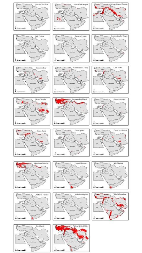
Considering the area of suitable habitats for the studied species, this study showed that Lebanon, Palestine, Turkey, and Israel face the highest risk of
biological invasion by the species on the whole. We ranked countries in the Middle East in the order of highest to lowest risk of biological invasion (Fig 2a). We
also ranked the studied species based on their risk of biological invasion; accordingly, African Spurred Tortoise, Veiled Chameleon, and Yellow Bellied Slider
had the highest risk of spreading in this area (Fig 2b).
Discussion And Conclusion
The results revealed the significant role of climatic and land cover/land use variables in determining the suitable habitat for the studied species. Our results
are in line with findings by similar studies in other regions such as the Zagros Mountains, western Iran (Hosseinzadeh et al., 2017), South Central USA (Salas
et al., 2017), Northwest China (Xu, 2015), North Africa (Martínez-Freiría et al., 2013), Egypt (El-Gabbas et al., 2016), northern Mexico (Gadsden et al., 2012), and
India (Rakholia et al., 220).
Our results indicate that all Middle Eastern countries included suitable habitats for at least six species, except Qatar, Kuwait and Bahrain for which the models
did not predict any suitable habitats. Our study showed that Lebanon, Palestine, Turkey, and Israel face the highest risk of biological invasion by the species
on the whole (Fig. 2a). Previous studies in these countries have not paid much attention to the invasion and trade of non-native reptiles, which makes the
management and conservation of these species difficult or even impossible. Also, the results showed that African Spurred Tortoise, Veiled Chameleon, and
Yellow Bellied Slider posed the highest risk of spreading in this area (Fig. 2b). Although these species have limited global range, their ability to spread in other
parts of the word should be taken into consideration.
The Veiled Chameleon is natively found in Saudi Arabia and Yemen, mostly in plateaus and grasslands (Showler, 1995; Schmidt, 2001). The species has been
introduced in Hawaii (Kraus and Duvall, 2004; Kraus 2009) and Florida (Gillette and Krysko, 2012; Edwards et al., 2014; Dalaba et al., 2019) in the United
States, where it is now commonly found. The Yellow Bellied Slider naturally occurs in the Mississippi Valley, its range stretching from Illinois to the Gulf of
Mexico. In the last five decades, the Yellow Bellied Slider has been grown commercially in the US for pet trade, and grown turtles have been accidentally
released into urban and natural landscapes (Cadi, et al., 2004). The species has been reported from a number of countries including Australia (Burgin, 2006),
Brazil (Ferronato et al., 2009), France (Prévot-Julliard et al., 2007), Japan (Oi et al., 2012), and South Africa (Newbery, 1984). Due to its extensive global spread,
the species has been categorized as one of the 100 worst invasive species (ISSG, 2021). The African Spurred Tortoise ranks second among terrestrial turtles in
terms of size, and naturally occurs in the western parts of the Sahel region. Although it is a threatened species and its population has been in decline through
its range, little information is available about the causes of this decline. Researchers have pointed to competition with cattle, wildfires, and pet trade as the
possible drivers of the decline in its population (Petrozzi et al., 2018). Despite the species having been reported from other countries, it is not clear whether it
has been able to establish populations outside its native range.
Wildlife managers should pay attention to species potential of invasion when making decisions about the import of non-native species into their countries.
Although the model did not indicate any areas with a potential distribution for Amazon Tree Boa and Burmese Python, managers should exercise caution
when making decisions about these species as well, and refer to previous studies or conduct more detailed research to further assess the risks associated with
non-native species.
Page 4/14SDMs take into account only the bioclimatic realized niche of species, meaning that the model assumes the species is only able to establish in areas with a
similar climate to its native range (Kearney 2006). It is obvious that biotic and abiotic factors and their interactions can alter a species’ realized niche
(Broennimann et al., 2007). This leads to the generated niche predictions in the new environments being only rough approximations. Consequently, a
mismatch between bioclimatic conditions in the native and introduced range can lead models to underestimate the extent of suitable areas. Further studies
focusing on each species and utilizing a wider range of data with better accuracy, including biotic variables, abiotic variables, and their interactions are needed
to make more nuanced judgments about each species. Such studies would also benefit from a comparison with areas that have the studied species as
invasive species.
In the meantime, managers should not interpret the absence of suitable habitats for some of the studies species as a license for unrestricted import or
introduction. Thus, the findings of this study are mainly helpful as a basis for imposing restrictions on species for which a suitable habitat was found; our
findings should not be seen as justification for allowing the introduction of species or loosening regulations. However, SDMs can still serve as the first step in
understanding the biological invasion history of species (Silva Rocha et al., 2015). The results of the current model need refinement and further investigation
to clarify the role of different factors in determining species distributions. Future studies should address niche shift and resolve the most important factors
underlying species distribution.
Declarations
Ethics approval and consent to participate
Not applicable
Consent for publication
Not applicable
Availability of data and materials
Some or all data, models, or code that support the findings of this study are available from the corresponding author upon reasonable request.
Competing interests
Not applicable
Funding
Not applicable
Authors' contributions
Azita Farashi: Writing and modelling, Mohammad Alizadeh-Noughani: Writing
Acknowledgements
We thank Pourya sardari who provided the research idea. This work was supported by Ferdowsi university of Mashhad [grant number 52250].
References
1. Alhajeri BH, Fourcade Y. High correlation between species-level environmental data estimates extracted from IUCN expert range maps and from GBIF
occurrence data. J Biogeogr. 2019;46(7):1329–41.
2. Allouche O, Tsoar A, Kadmon R. Assessing the accuracy of species distribution models: prevalence kappa and the true skill statistic (TSS). Journal of
applied ecology. 2006;43(6):1223–32.
3. Araújo MB, New M. Ensemble forecasting of species distributions. Trends Ecol Evol. 2007;22(1):42–7.
4. Barbet-Massin M, Jiguet F, Albert CH, Thuiller W. Selecting pseudo‐absences for species distribution models: how, where and how many? Methods in
ecology evolution. 2012;3(2):327–38.
5. Bevan HR, Jenkins DG, Campbell TS. From pet to pest? Differences in ensemble SDM predictions for an exotic reptile using both native and nonnative
presence data. Frontiers of Biogeography. 2019;11(2):e42596.
6. Block C, Pedrana J, Stellatelli OA, Vega LE, Isacch JP. Habitat suitability models for the sand lizard Liolaemus wiegmannii based on landscape
characteristics in temperate coastal dunes in Argentina. Austral ecology. 2016;41(6):671–80.
7. Bomford M, Kraus F, Braysher M, Walter L, Brown L. Risk assessment model for the import and keeping of exotic reptiles and amphibians, A report
produced for the. Department of Environment and Heritage, Bureau of Rural Sciences Canberra; 2005. p. 110.
8. Breiman L. Random forests. Machine learning. 2001;45(1):5–32.
9. Broennimann O, Treier UA, Müller-Schärer H, Thuiller W, Peterson AT, Guisan A. Evidence of climatic niche shift during biological invasion. Ecology letters.
2007;10(8):701–9.
Page 5/1410. Brown JL. SDMtoolbox: a python-based GIS toolkit for landscape genetic, biogeographic and species distribution model analyses. Methods Ecol Evol.
2014;5(7):694–700.
11. Brown JL, Yoder AD. Shifting ranges and conservation challenges for lemurs in the face of climate change. Ecology Evolution. 2015;5(6):1131–42.
12. Burgin S. Confirmation of an established population of exotic turtles in urban Sydney. Australian Zoologist. 2006;33(3):379–84.
13. Burridge MJ, Simmons LA, Allan SA. Introduction of potential heart water vectors and other exotic ticks into Florida on imported reptiles. J Parasitol.
2000;86(4):700–4.
14. Busby J. BIOCLIM-a bioclimate analysis and prediction system. Plant protection quarterly (Australia); 1991.
15. Bush ER, Baker SE, Macdonald DW. Global trade in exotic pets 2006–2012. Conserv Biol. 2014;28(3):663–76.
16. Cadi A, Delmas V, Prévot-Julliard AC, Joly P, Pieau C, Girondot M. Successful reproduction of the introduced slider turtle (Trachemys scripta elegans) in the
South of France. Aquatic conservation: Marine Freshwater ecosystems. 2004;14(3):237–46.
17. Capinha C, Seebens H, Cassey P, García-Díaz P, Lenzner B, Mang T, … Winter M. Diversity, biogeography and the global flows of alien amphibians and
reptiles. Divers Distrib. 2017;23(11):1313–22.
18. Choudhary JS, Mali SS, Fand BB, Das B. Predicting the invasion potential of indigenous restricted mango fruit borer, Citripestis eutraphera (Lepidoptera:
Pyralidae) in India based on MaxEnt modelling. Curr Sci. 2019;116(4):636.
19. Cordier JM, Loyola R, Rojas-Soto O, Nori J. Modeling invasive species risk from established populations: Insights for management and conservation.
Perspectives in Ecology Conservation. 2020;18(2):132–8.
20. Dalaba JR, Rochford MR, Metzger EF, Gillette CR, Schwartz NP, Gati EV, … Mazzotti FJ. New county records for introduced reptiles in St. Lucie County,
Florida, with some observations on diets. Reptiles Amphibians. 2019;26(2):155–8.
21. Dormann CF, Calabrese JM, Guillera-Arroita G, Matechou E, Bahn V, Bartoń K, … Hartig F. Model averaging in ecology: A review of Bayesian, information‐
theoretic, and tactical approaches for predictive inference. Ecol Monogr. 2018;88(4):485–504.
22. Edwards JR, Rochford MR, Mazzotti FJ, Krysko KL. New county record for the veiled chameleon (Chamaeleo calyptratus Dumeril and Bibron 1851), in
Broward County, Florida, with notes on intentional introductions of chameleons in southern Florida. Reptiles Amphibians. 2014;21(2):83–5.
23. El-Gabbas A, El Din SB, Zalat S, Gilbert F. Conserving Egypt's reptiles under climate change. J Arid Environ. 2016;127:211–21.
24. Elith J, Leathwick JR. Species distribution models: ecological explanation and prediction across space and time. Annual review of ecology evolution
systematics. 2009;40:677–97.
25. Elith J, Leathwick JR, Hastie T. A working guide to boosted regression trees. J Anim Ecol. 2008;77(4):802–13.
26. Elith J, Phillips SJ, Hastie T, Dudík M, Chee YE, Yates CJ. A statistical explanation of MaxEnt for ecologists. Diversity distributions. 2011;17(1):43–57.
27. Ferronato BO, Marques TS, Guardia I, Longo AL, Piña CI, Bertoluci J, Verdade LM. (2009). The turtle Trachemys scripta elegans (Testudines, Emydidae) as
an invasive species in a polluted stream of southeastern Brazil, 109, (29–34).
28. Franklin J. Mapping species distributions: spatial inference and prediction. Cambridge University Press; 2010.
29. Friedman JH. 1991. Multivariate adaptive regression splines. The annals of statistics 1–67.
30. Gadsden H, Ballesteros-Barrera C, de la Garza OH, Castañeda G, García-De la Peña C., Lemos-Espinal JA. 2012. Effects of land-cover transformation and
climate change on the distribution of two endemic lizards Crotaphytus antiquus and Sceloporus cyanostictus of northern Mexico. Journal of arid
environments 83:1–9.
31. García-Díaz P, Ross JV, Woolnough AP, Cassey P. The illegal wildlife trade is a likely source of alien species. Conservation Letters. 2017;10(6):690–8.
32. Gillette CR, Krysko KL. New county record for the Veiled Chameleon, Chamaeleo calyptratus Duméril and Bibron 1851 (Sauria: Chamaeleonidae), in
Florida. Reptiles Amphibians. 2012;19(2):130–1.
33. Guisan A, Edwards TC, Hastie T. 2002. Generalized linear and generalized additive models in studies of species distributions: setting the scene. Ecological
modelling 157(2).
34. Guisan A, Thuiller W. Predicting species distribution: offering more than simple habitat models. Ecology letters. 2005;8(9):993–1009.
35. Guisan A, Thuiller W, Zimmermann NE. Habitat suitability and distribution models: with applications in R. Cambridge University Press; 2017.
36. Hastie T, Tibshirani R, Buja A. Flexible discriminant analysis by optimal scoring. Journal of the American statistical association. 1994;89(428):1255–70.
37. Hijmans RJ, Cameron SE, Parra JL, Jones PG, Jarvis A. Very high resolution interpolated climate surfaces for global land areas. International journal of
climatology. 2005;25(15):1965–78.
38. Holbrook J, Chesnes T. 2011. An effect of Burmese pythons (Python molurus bivittatus) on mammal populations in southern Florida. Florida Scientist
17–24.
39. Hosseinzadeh MS, Ghezellou P, Kazemi SM. Predicting the potential distribution of the endemic snake Spalerosophis microlepis (Serpentes: Colubridae):
in the Zagros Mountains western Iran. Salamandra. 2017;53(2):294–8.
40. Hulme PE. Invasion pathways at a crossroad: policy and research challenges for managing alien species introductions. J Appl Ecol. 2015;52(6):1418–24.
41. ISSG. (2021). (Invasive Species Specialist Group, International Union for the Conservation of Nature) Global Invasive Species Data Base. (Accessed: April
2021).
42. Jha KK, Jha R. Study of Vulture Habitat Suitability and Impact of Climate Change in Central India Using MaxEnt. Journal of Resources Ecology.
2021;12(1):30–42.
43. Kalboussi M, Achour H. Modelling the spatial distribution of snake species in northwestern Tunisia using maximum entropy (Maxent) and Geographic
Information System (GIS). Journal of Forestry Research. 2018;29(1):233–45.
Page 6/1444. Karesh WB, Cook RA, Bennett EL, Newcomb J. Wildlife trade and global disease emergence. Emerg Infect Dis. 2005;11(7):1000.
45. Kearney M. Habitat environment and niche: what are we modelling? Oikos. 2006;115(1):186–91.
46. Keller RP, Lodge DM, Finnoff DC. 2007. Risk assessment for invasive species produces net bioeconomic benefits. Proceedings of the National Academy of
Sciences 104(1): 203–207.
47. Kraus F. Impacts from invasive reptiles and amphibians. Annu Rev Ecol Evol Syst. 2015;46:75–97.
48. Lek S, Guégan JF. Artificial neural networks as a tool in ecological modelling an introduction. Ecological modelling. 1999;120(2):65–73.
49. Luiselli L, Bonnet X, Rocco M, Amori G. Conservation implications of rapid shifts in the trade of wild African and Asian pythons. Biotropica.
2012;44(4):569–73.
50. Martínez-Freiría F, Argaz H, Fahd S, Brito JC. Climate change is predicted to negatively influence Moroccan endemic reptile richness, Implications for
conservation in protected areas. Naturwissenschaften. 2013;100(9):877–89.
51. Merow C, Smith MJ, Edwards TC, Guisan A, McMahon SM, Normand S, … Elith J. 2014. What do we gain from simplicity versus complexity in species
distribution models?. Ecography 37(12): 1267–1281.
52. Newbery R. The American red-eared terrapin in South Africa. African Wildlife. 1984;38(5):186–9.
53. Nowak M. The international trade in reptiles (Reptilia)—the cause of the transfer of exotic ticks (Acari: Ixodida) to Poland. Veterinary parasitology.
2010;169(3–4):373–81.
54. Oi M, Araki J, Matsumoto J, Nogami S. Helminth fauna of a turtle species introduced in Japan, the red-eared slider turtle (Trachemys scripta elegans). Res
Vet Sci. 2012;93(2):826–30.
55. Parolo G, Rossi G, Ferrarini A. Toward improved species niche modelling: Arnica montana in the Alps as a case study. J Appl Ecol. 2008;45(5):1410–8.
56. Petrozzi F, Eniang EA, Akani GC, Amadi N, Hema EM, Diagne T, … Luiselli L. Exploring the main threats to the threatened African spurred tortoise
Centrochelys sulcata in the West African Sahel. Oryx. 2018;52(3):544–51.
57. Phillips SJ, Anderson RP, Schapire RE. Maximum entropy modeling of species geographic distributions. Ecological modelling. 2006;190(3):231–59.
58. Prévot-Julliard AC, Gousset E, Archinard C, Cadi A, Girondot M. Pets and invasion risks: is the slider turtle strictly carnivorous? Amphibia-Reptilia.
2007;28(1):139–43.
59. Pyšek P, Richardson DM, Pergl J, Sixtova JV, Weber Z E. Geographical and taxonomic biases in invasion ecology. Trends in Ecology Evolution.
2008;23(5):237–44.
60. Rakholia S, Mehta A, Suthar B. Forest fire monitoring of Shoolpaneshwar Wildlife Sanctuary, Gujarat, India using geospatial techniques. Curr Sci.
2020;119(12):1974–81.
61. Rangel TFL, Diniz-Filho JAF, Bini LM. Towards an integrated computational tool for spatial analysis in macroecology and biogeography. Global ecology
biogeography. 2006;15(4):321–7.
62. Rastegar-Pouyani N, Gholamifard A, Karamiani R, Bahmani Z, Mobaraki A, Abtin E, … Ahsani N. Sustainable management of the herpetofauna of the
Iranian Plateau and coastal Iran. Amphibian Reptile Conservation. 2015;9(1):1–15.
63. Reed RN. An ecological risk assessment of nonnative boas and pythons as potentially invasive species in the United States. Risk Anal. 2005;25(3):753–
66.
64. Ribeiro-Júnior M, Amaral S. Diversity, distribution, and conservation of lizards (Reptilia: Squamata) in the Brazilian Amazonia. Neotropical Biodiversity.
2016;2(1):195–421.
65. Salas EAL, Seamster VA, Harings NM, Boykin KG, Alvarez G, Dixon KW. Projected Future Bioclimate-Envelope Suitability for Reptile and Amphibian Species
of Concern in South Central USA. Herpetological Conservation Biology. 2017;12(2):522–47.
66. Sanchooli N. Habitat suitability and potential distribution of Laudakia nupta (De Filippi, 1843) (Sauria: Agamidae) in Iran. Russian Journal of Ecology.
2017;48(3):275–9.
67. Savidge JA. Extinction of an island forest avifauna by an introduced snake. Ecology. 1987;68(3):660–8.
68. Schmidt W. Chamaeleo calyptratus, the Yemen Chameleon. Berlin: Matthias Schmidt Publications, Natur und Tier-Verlag; 2001.
69. Segurado P, Araujo MB. An evaluation of methods for modelling species distributions. Journal of biogeography. 2004;31(10):1555–68.
70. Seni G, Elder JF. Ensemble methods in data mining: improving accuracy through combining predictions. Synthesis lectures on data mining knowledge
discovery. 2010;2(1):1–126.
71. Showler DA. (1995). Reptile observations in Yemen, March-May 1993. BULLETIN-BRITISH HERPETOLOGICAL SOCIETY, 13–23.
72. Silva Rocha I, Salvi D, Sillero N, Mateo JA, Carretero MA. Snakes on the Balearic Islands: an invasion tale with implications for native biodiversity
conservation. PloS one. 2015;10(4):e0121026.
73. Soorae PS, Al Quarqaz M, Gardner AS. An overview and checklist of the native and alien herpetofauna of the Emirates. Herpetological Conservation
Biology. 2010;5(3):529–36.
74. Stringham OC, Lockwood JL. Pet problems: biological and economic factors that influence the release of alien reptiles and amphibians by pet owners. J
Appl Ecol. 2018;55(6):2632–40.
75. Thuiller W, Georges D, Engler R. 2014. biomod2: Ensemble platform for species distribution modeling, R package version 3,1–64, Availablt at: http://CRAN,
R-project, org/package = biomod2 (accessed February 2015).
76. Thuiller W, Lafourcade B, Engler R, Araújo MB. BIOMOD–a platform for ensemble forecasting of species distributions. Ecography. 2009;32(3):369–73.
Page 7/1477. Vayssières MP, Plant RE, Allen-Diaz BH. Classification trees: An alternative non‐parametric approach for predicting species distributions. Journal of
vegetation science. 2000;11(5):679–94.
78. Xu Z. Potential distribution of invasive alien species in the upper Ili river basin: determination and mechanism of bioclimatic variables under climate
change. Environ Earth Sci. 2015;73(2):779–86.
79. Zimmermann NE, Edwards TC Jr, Graham CH, Pearman PB, Svenning JC. New trends in species distribution modelling. Ecography. 2010;33(6):985–9.
Tables
Table 1
Pearson correlation coefficient matrix of environmental variables (values in bold are r > 0.70 and r <
Variable C19 C18 C17 C16 C15 C14 C13 C12 C11 C10 C9 C8 C7 C6 C5 C4 C3 C2
C19
C18 0.34
C17 0.67 0.55
C16 0.50 0.77 0.39
C15 -0.29 -0.09 -0.52 0.16
C14 0.65 0.53 0.99 0.36 -0.51
C13 0.47 0.74 0.35 0.99 0.21 0.32
C12 0.68 0.82 0.71 0.91 -0.14 0.68 0.87
C11 0.19 0.13 0.01 0.38 0.42 -0.01 0.38 0.30
C10 -0.13 -0.20 -0.28 -0.02 0.48 -0.28 0.01 -0.15 0.71
C9 0.15 -0.11 -0.06 0.15 0.29 -0.08 0.16 0.10 0.84 0.74
C8 -0.12 0.17 -0.12 0.20 0.47 -0.13 0.22 0.09 0.58 0.62 0.24
C7 -0.42 -0.41 -0.32 -0.59 -0.12 -0.29 -0.58 -0.61 -0.79 -0.17 -0.56 -0.30
C6 0.24 0.20 0.08 0.43 0.37 0.06 0.44 0.37 0.99 0.65 0.82 0.56 -0.85
C5 -0.21 -0.27 -0.35 -0.11 0.51 -0.35 -0.08 -0.25 0.64 0.98 0.69 0.72 -0.05 0.56
C4 -0.33 -0.30 -0.19 -0.52 -0.25 -0.17 -0.51 -0.50 -0.89 -0.32 -0.66 -0.39 0.96 -0.92 -0.24
C3 0.07 0.05 0.03 0.10 0.07 0.03 0.10 0.09 0.18 0.12 0.14 0.12 -0.14 0.17 0.11 -0.17
C2 -0.36 -0.76 -0.46 -0.37 0.44 -0.45 -0.35 -0.50 0.24 0.52 0.31 0.26 0.28 0.12 0.67 0.01 0.08
C1 0.07 0.03 -0.10 0.26 0.48 -0.11 0.27 0.16 0.96 0.87 0.85 0.65 -0.62 0.64 0.66 -0.64 0.17 0.3
TMS 0.01 0.03 0.01 0.03 0.03 0.01 0.03 0.03 0.03 0.01 0.01 0.03 0.00 0.01 0.03 -0.03 0.02 0.1
TSS 0.01 0.03 0.01 0.03 0.03 0.01 0.03 0.03 0.03 0.01 0.01 0.03 0.00 0.01 0.03 -0.03 0.02 0.1
TME -0.10 -0.05 -0.14 -0.06 0.11 -0.14 -0.06 -0.09 -0.10 -0.20 -0.09 -0.17 0.08 -0.13 -0.11 0.01 0.04 0.2
TSE -0.10 -0.05 -0.14 -0.06 0.11 -0.14 -0.06 -0.09 -0.10 -0.20 -0.09 -0.17 0.08 -0.13 -0.11 0.01 0.04 0.2
LV 0.00 0.00 0.00 0.00 0.00 0.00 0.00 0.00 0.00 0.00 0.00 0.00 0.00 0.00 0.00 0.00 0.00 0.0
NDVI 0.06 0.03 0.00 0.30 0.71 -0.70 0.29 0.20 0.43 0.67 0.51 0.50 -0.41 0.64 0.71 -0.70 0.12 0.3
HFI 0.00 0.00 0.00 0.00 0.00 0.00 0.00 0.00 0.00 0.00 0.00 0.00 0.00 0.00 0.00 0.00 0.00 0.0
Climatic variables: C1 (Annual Mean Temperature), C2 (Mean Diurnal Range), C3 (Isothermality), C4 (Temperature Seasonality), C5 (Max Temperature of War
(Temperature Annual Range), C8 (Mean Temperature of Wettest Quarter), C9 (Mean Temperature of Driest Quarter), C10 (Mean Temperature of Warmest Qua
Precipitation), C13 (Precipitation of Wettest Month), C14 (Precipitation of Driest Month), C15 (Precipitation Seasonality), C16 (Precipitation of Wettest Quarte
Warmest Quarter), C19 (Precipitation of Coldest Quarter)
Topographic variables: TME (Mean of the Elevation), TSE (Standard Deviation of the Elevation), TMS (Mean of the Slope), TSS (Standard Deviation of the Slo
Land cover/land use variables: LV (Land Cover), NDVI (Normalized Difference Vegetation Index), HFI (Human Footprint Index)
Selected variables to model: C1, C3, C4, C5, C12, C16, C17, C18, C19, TME, TMS, LV, NDVI, HFI
Page 8/14Table 2
Studied reptile species and the three most important environmental variables that determine their potential geographic distributions.
Scientific name Common name Statues The number of presence Important environmental
points variables
IUCN CITES (Relative contribution, %)
Anolis carolinensis (Voigt, 1832) Green Anole LC - 9938 C17 C3 (10) TME (9)
(60)
Astrochelys radiate (Shaw, 1802) Radiated Tortoise CR I 62 C18 C3 (30) C4 (10)
(40)
Boa constrictor (Linnaeus, 1758) Common Boa DD II 585 C12 C6 (39) C16
(40) (11)
Centrochelys sulcata (Miller, 1779) African Spurred VU II 89 NDVI C12 NDVI
Tortoise (35) (28) (17)
Chamaeleo calyptratus (Duméril & Bibron, Veiled Chameleon LC II 84 C19 C3 (18) C12
1851) (54) (10)
Corallus hortulanus (Linnaeus, 1758) Amazon Tree Boa LC II 102 C4 (52) NDVI C12
(19) (11)
Emys orbicularis (Linnaeus, 1758) European Pond Turtle NT - 1136 C1 (47) C12 C4 (8)
(20)
Eunectes murinus (Linnaeus, 1758) Green Anaconda DD - 80 C19 C4 (20) NDVI
(49) (10)
Glyptemys insculpta (Le Conte, 1830) Wood Turtle EN II 344 C16 C17 C19
(32) (19) (11)
Gopherus agassizii (Cooper, 1863) Desert Tortoise VU II 614 C1 (51) C6 (21) C5 (9)
Iguana iguana (Linnaeus, 1758) Green Iguana DD II 4114 C6 (50) C4 (22) TME (5)
Morelia viridis (Schlegel, 1872) Green Tree Python LC II 134 C18 C4 (14) C1 (8)
(44)
Pantherophis guttatus (Linnaeus, 1766) Corn Snake LC - 667 C17 C16 TME (7)
(45) (28)
Physignathus Cocincinus (Cuvier, 1829) Asian Water Dragon DD - 60 C12 NDVI C18 (8)
(45) (30)
Pogona barbata (Cuvier, 1829) Common Bearded LC - 1921 C4 (48) C3 (26) C6 (11)
Dragon
Python bivittatus (Kuhl, 1820) Burmese Python VU II 855 C18 C6 (32) C4 (8)
(46)
Python regius (Shaw, 1802) Ball Python LC II 347 C19 C12 NDVI
(41) (30) (12)
Python reticulatus (Schneider, 1801) Reticulated Python DD II 51 C6 (51) C4 (31) C1 (7)
Stigmochelys pardalis (Bell, 1828) Leopard Tortoise LC II 308 C3 (49) C18 C1 (7)
(14)
Terrapene carolina (Linnaeus, 1758) Common Box Turtle VU II 7854 C17 C12 NDVI (5)
(61) (15)
Testudo hermanni (Gmelin, 1789) Hermann’s Tortoise NT II 498 C1 (51) C12 C19 (5)
(13)
Trachemys scripta (Thunberg in Schoepff, Yellow Bellied Slider LC - 9055 NDVI C12 NDVI
1792) (50) (19) (12)
Varanus niloticus (Linnaeus, 1766) Nile Monitor DD II 660 C3 (34) C4 (21) NDVI (8)
IUCN Red List Categories: CR (Critically Endangered), EN (Endangered), VU (Vulnerable), NT (Near Threatened), LC (Least Concern), and DD (Data
Deficient).
CITES Appendices: I (it lists species that are the most endangered among CITES-listed animals and plants), and II (it lists species that are not necessarily
now threatened with extinction but that may become so unless trade is closely controlled).
Page 9/14Table 3
The species distribution models in Biomod2 used in this research and their required type of dependent variables
Group Algorithms Replicates Runs Number of pseudo-absences
1 Artificial neural networks (ANN) (Lek and Guegan, 1999) 5 10 1000
Surface range envelope (SRE) (Busby, 1991)
Generalized additive models (GAM) (Guisan et al., 2002)
Generalized linear models (GLM) (Guisan et al., 2002)
Maximum entropy (MaxEnt) (Phillips et al., 2006)
2 Random forest (RF) (Breiman, 2001) 5 10 1000
Boosted regression trees (BRT) (Elith et al., 2008)
Classification and regression trees (CART) (Vayssieres et al., 2000)
3 Flexible discriminant analysis (FDA) (Hastie et al., 1994) 7 10 100
Multivariate adaptive regression splines (MARS) (Friedman, 1991)
Page 10/14Table 4
Accuracy metrics for all models (SEN: sensitivity, SPE: specificity, T
Species ANN SRE GAM GLM MaxEnt RF B
SEN SPE TSS SEN SPE TSS SEN SPE TSS SEN SPE TSS SEN SPE TSS SEN SPE TSS S
Green 0.76 0.73 0.81 0.70 0.70 0.71 0.81 0.77 0.70 0.88 0.73 0.81 0.82 0.83 0.71 0.74 0.75 0.73 0
Anole
Radiated 0.84 0.72 0.88 0.66 0.70 0.73 0.81 0.90 0.90 0.85 0.90 0.73 0.80 0.73 0.92 0.73 0.70 0.80 0
Tortoise
Common 0.81 0.90 0.83 0.72 0.59 0.73 0.92 0.72 0.76 0.72 0.84 0.85 0.69 0.80 0.78 0.91 0.72 0.72 0
Boa
African 0.85 0.72 0.85 0.59 0.70 0.72 0.90 0.89 0.89 0.76 0.69 0.89 0.72 0.65 0.82 0.69 0.89 0.74 0
Spurred
Tortoise
Veiled 0.82 0.84 0.81 0.70 0.70 0.73 0.81 0.76 0.84 0.66 0.84 0.81 0.89 0.70 0.73 0.80 0.85 0.81 0
Chameleon
Amazon 0.85 0.70 0.90 0.59 0.65 0.72 0.83 0.69 0.89 0.69 0.76 0.81 0.65 0.84 0.70 0.84 0.66 0.74 0
Tree Boa
European 0.73 0.84 0.78 0.76 0.70 0.72 0.79 0.70 0.76 0.85 0.85 0.92 0.85 0.72 0.72 0.89 0.73 0.74 0
Pond
Turtle
Green 0.81 0.73 0.83 0.65 0.59 0.73 0.88 0.81 0.81 0.66 0.65 0.84 0.80 0.66 0.73 0.69 0.70 0.74 0
Anaconda
Wood 0.73 0.85 0.83 0.70 0.70 0.72 0.90 0.73 0.75 0.65 0.80 0.75 0.81 0.85 0.85 0.72 0.66 0.85 0
Turtle
Desert 0.72 0.76 0.81 0.59 0.69 0.70 0.80 0.65 0.84 0.81 0.76 0.73 0.81 0.66 0.76 0.65 0.81 0.74 0
Tortoise
Green 0.84 0.70 0.82 0.65 0.70 0.79 0.83 0.76 0.73 0.73 0.89 0.76 0.77 0.70 0.77 0.89 0.89 0.72 0
Iguana
Green Tree 0.81 0.72 0.92 0.65 0.70 0.70 0.83 0.80 0.89 0.80 0.81 0.89 0.76 0.76 0.81 0.70 0.76 0.74 0
Python
Corn 0.82 0.81 0.91 0.77 0.59 0.72 0.84 0.72 0.80 0.82 0.73 0.76 0.80 0.70 0.70 0.66 0.77 0.76 0
Snake
Asian 0.70 0.73 0.93 0.72 0.70 0.75 0.65 0.65 0.72 0.66 0.77 0.72 0.65 0.89 0.72 0.85 0.84 0.92 0
Water
Dragon
Common 0.73 0.82 0.88 0.72 0.70 0.73 0.85 0.66 0.85 0.84 0.72 0.77 0.84 0.85 0.89 0.69 0.70 0.80 0
Bearded
Dragon
Burmese 0.84 0.73 0.83 0.59 0.66 0.72 0.65 0.81 0.73 0.77 0.73 0.84 0.89 0.69 0.70 0.72 0.73 0.72 0
Python
Ball 0.72 0.73 0.84 0.70 0.70 0.73 0.81 0.65 0.90 0.72 0.80 0.89 0.80 0.72 0.76 0.80 0.90 0.84 0
Python
Reticulated 0.81 0.72 0.81 0.69 0.59 0.72 0.65 0.80 0.84 0.65 0.65 0.72 0.69 0.66 0.92 0.82 0.89 0.74 0
Python
Leopard 0.72 0.81 0.80 0.72 0.76 0.73 0.84 0.73 0.90 0.73 0.72 0.92 0.82 0.65 0.73 0.90 0.72 0.92 0
Tortoise
Common 0.73 0.69 0.90 0.69 0.72 0.76 0.65 0.70 0.70 0.77 0.76 0.76 0.89 0.76 0.89 0.76 0.90 0.85 0
Box Turtle
Hermann’s 0.84 0.70 0.85 0.70 0.69 0.73 0.73 0.69 0.90 0.73 0.77 0.73 0.73 0.73 0.76 0.90 0.73 0.80 0
Tortoise
Yellow 0.73 0.70 0.79 0.59 0.70 0.72 0.70 0.77 0.81 0.69 0.70 0.70 0.81 0.70 0.73 0.84 0.69 0.92 0
Bellied
Slider
Nile 0.89 0.77 0.75 0.70 0.77 0.73 0.77 0.89 0.77 0.89 0.80 0.77 0.89 0.90 0.80 0.90 0.77 0.89 0
Monitor
Page 11/14Table 5
The areas of suitable habitats for studied species (the highest values are in bold).
Species Suitable habitats for studied species
Emirates Egypt Iran Iraq Israel Jordan Lebanon Oman Palestine Saudi Syri
Arabia
Green Km2 38.59 0 24368.84 34.25 0 0 3156.97 38.53 0 0 139
Anole
% 0.05 0 1.50 0.01 0 0 31.53 0.01 0 0 7.52
Radiated Km2 0 0 0 0 0 0 0 0 0 0 0
Tortoise
% 0 0 0 0 0 0 0 0 0 0 0
Common Km2 38.59 0 19987.60 0 380.57 108.39 1225.33 1990.37 127.99 0 426
Boa
% 0.05 0 1.23 0 1.71 0.12 12.24 0.64 2.05 0 2.30
African Km2 57.91 39047.87 166030.71 53941.71 18415.04 21219.85 9391.26 2757.50 6057.29 1646.56 338
Spurred
Tortoise % 0.08 3.91 10.25 12.36 82.72 23.88 93.80 0.89 97.08 0.09 18.2
Veiled Km2 4171.19 4873.81 232053.38 2958.64 11803.12 8830.22 6469.14 25438.67 5511.16 104402.26 203
Chameleon
% 5.85 0.49 14.32 0.68 53.02 9.94 64.62 8.17 88.33 5.43 10.9
Amazon Km2 0 0 0 0 0 0 0 0 0 0 0
Tree Boa
% 0 0 0 0 0 0 0 0 0 0 0
European Km2 0 454.49 90487.52 0 0 0 3119.83 59.06 0 58.94 911
Pond
Turtle % 0 0.05 5.59 0 0 0 31.16 0.02 0 0.00 4.91
Green Km2 57.91 54.87 648.52 0 1756.87 0 2896.81 250.61 146.22 0 175
Anaconda
% 0.08 0.01 0.04 0 7.89 0 28.93 0.08 2.34 0 0.95
Wood Km2 0 0 0 0 0 0 0 0 0 0 0
Turtle
% 0 0 0 0 0 0 0 0 0 0 0
Desert Km2 0 0 216799.14 0 0 0 0 433.52 0 560.12 433
Tortoise
% 0 0 13.38 0 0 0 0 0.14 0 0.03 0.23
Green Km2 0 0 1185.07 0 0 0 2149.38 1308.34 0 1122.11 131
Iguana
% 0 0 0.07 0 0 0 21.47 0.42 0 0.06 0.71
Green Tree Km2 1774.32 677.79 38632.42 0 3623.75 1992.91 106.81 329.73 1459.78 780.48 89.7
Python
% 2.49 0.07 2.38 0 16.28 2.24 1.07 0.11 23.40 0.04 0.05
Corn Km2 0 0 25860.74 0 0 0 1821.93 253.31 0 0 126
Snake
% 0 0 1.60 0 0 0 18.20 0.08 0 0 6.82
Asian Km2 0 33725.08 3612.00 0 0 0 0 79.07 0 0 0
Water
Dragon % 0 3.37 0.22 0 0 0 0 0.03 0 0 0
Common Km2 0 0 996.29 0 0 0 0 2504.10 18.28 1152.75 0
Bearded
Dragon % 0 0 0.06 0 0 0 0 0.80 0.29 0.06 0
Burmese Km2 0 0 0 0 0 0 0 0 0 0 0
python
% 0 0 0 0 0 0 0 0 0 0 0
Ball Km2 0 0 532.52 0 468.76 126.47 106.62 134.91 0 0 123
Python
% 0 0 0.03 0 2.11 0.14 1.06 0.04 0 0 0.07
Reticulated Km2 0 0 0 0 0 0 0 0 0 0 0
Python
% 0 0 0 0 0 0 0 0 0 0 0
Leopard Km2 0 36.85 125.05 0 941.00 90.31 0 511.91 181.38 8691.56 0
Tortoise
Page 12/14% 0 0.00 0.01 0 4.23 0.10 0 0.16 2.91 0.45 0
Common Km2 0 0 2416.07 102.35 0 0 88.39 117.45 0 0 140
Box Turtle
% 0 0 0.15 0.02 0 0 0.88 0.04 0 0 0.76
Hermann’s Km2 0 0 28835.95 0 287.80 0 2881.39 0 0 0 452
Tortoise
% 0 0 1.78 0 1.29 0 28.78 0 0 0 2.44
Yellow Km2 77.22 0 614677.89 8218.48 2442.59 7977.13 6393.26 5340.91 4131.13 12577.05 310
Bellied
Slider % 0.11 0 37.94 1.88 10.97 8.98 63.86 1.72 66.21 0.65 16.7
Nile Km2 0 0 0 0 0 0 0 415.05 0 0 0
Monitor
% 0 0 0 0 0 0 0 0.13 0 0 0
Figures
Figure 1
Potential distribution map of the studied species in the world (red: suitable habitats, gray: unsuitable habitats)
Page 13/14Figure 2
The areas of suitable habitats for countries (a) and studied species (b).
Page 14/14You can also read