PROCEEDINGS OF SPIE Integrating bias and gain invariance with the generalized Anscombe transform for wavefront sensing - University of Rochester ...
←
→
Page content transcription
If your browser does not render page correctly, please read the page content below
PROCEEDINGS OF SPIE
       SPIEDigitalLibrary.org/conference-proceedings-of-spie

                   Integrating bias and gain invariance
                   with the generalized Anscombe
                   transform for wavefront sensing

                   Tang, Joseph, Fienup, James

                                  Joseph S. Tang, James R. Fienup, "Integrating bias and gain invariance with
                                  the generalized Anscombe transform for wavefront sensing," Proc. SPIE
                                  11443, Space Telescopes and Instrumentation 2020: Optical, Infrared, and
                                  Millimeter Wave, 1144348 (13 December 2020); doi: 10.1117/12.2562416

                                  Event: SPIE Astronomical Telescopes + Instrumentation, 2020, Online Only

Downloaded From: https://www.spiedigitallibrary.org/conference-proceedings-of-spie on 14 Jan 2021 Terms of Use: https://www.spiedigitallibrary.org/terms-of-use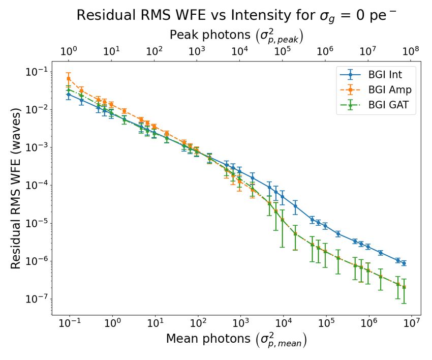
Integrating bias and gain invariance with the generalized
                             Anscombe transform for wavefront sensing
                                                             Joseph S. Tang and James R. Fienup
                                   Institute of Optics, University of Rochester, Rochester, NY USA 14620

                                                                                 ABSTRACT
                In image-based wavefront sensing by phase retrieval, the sum-squared difference (SSD) of simulated and measured
                PSF intensities, i.e., the intensity error metric (IEM), suffers from noise model mismatch. The IEM assumes
                additive Gaussian noise, but the true noise model is mixed Poisson-Gaussian (PG). The generalized Anscombe
                transform (GAT) addresses this issue by transforming the noise model from mixed PG to approximately additive
                Gaussian. We developed a method that uses the bias and gain terms derived for the bias-and-gain-invariant
                (BGI) IEM to create a BGI GAT error metric (GEM) and a BGI SSD of field amplitudes, i.e., amplitude error
                metric (AEM). We performed simulations comparing the retrieval accuracy of the three BGI metrics for various
                amounts of mixed PG noise. We found that the BGI GEM performs comparable or better than the BGI IEM
                and AEM for all amounts of mixed PG noise. Therefore, the BGI GEM is a good general-use error metric that
                works well for any mixed PG noise.
                Keywords: phase retrieval, wavefront sensing, bias and gain invariant, generalized Anscombe transform

                                                                          1. INTRODUCTION
                When performing image-based wavefront sensing using phase retrieval by nonlinear optimization, a simulated
                point-spread function (PSF), I, is calculated from a exit pupil wavefront estimate and compared to a measured
                data PSF, D, using an error metric, and the calculated error is used to refine the pupil wavefront estimate via
                nonlinear optimization. The error metric used is important because it can affect the accuracy and convergence
                rate of the retrieved wavefront. A highly desired property for an error metric is bias and gain invariance, i.e., the
                error metric is invariant to bias and gain errors between the simulated and data PSF.1 Bias and gain invariance
                allows for faster testing, as it removes the need for calibration steps needed to account for these factors and gives
                a more accurate estimate when the calibration is imperfect.
                    To emphasize the importance of bias and gain invariance, we can look at the history of error metrics used for
                phase retrieval by nonlinear optimization. Two error metrics that are most common that we will focus on are 1)
                the sum-squared difference in image field amplitude (i.e., magnitude, the square root of the PSF intensities),2
                and 2) the sum-squared difference in PSF intensities.3, 4 We will call the first error metric the amplitude error
                metric (AEM), and the second the intensity error metric (IEM). Initially, the AEM was preferred over the IEM
                for many reasons,3 but for now it will suffice to say that it is because the AEM would perform better than the
                IEM in some cases (which we will explain later). We will give the intuitive reason here first, but we will give a
                mathematical explanation later in this section. Intuitively, as the intensity increases, the variance of the Poisson
                noise also increases, and thus even though higher intensity pixels have higher signal-to-noise ratio (SNR), they
                also have more Poisson noise. Therefore, if in an error metric the intensity at each pixel is inversely weighted
                by the variance of the noise at that pixel, which is reasonable, then higher intensity pixels should be weighted
                less than lower intensity pixels. This is why the AEM may perform better than the IEM, because in effect the
                square root enforces this sort of relative weighting on the pixels. Connected with that, the AEM was known to
                give an approximately maximum likelihood estimate for a Poisson noise model and the IEM was known to give
                the maximum likelihood estimate for additive Gaussian noise, as described in Ref. 4. Then, in 2009, Thurman
                developed a bias-and-gain-invariant (BGI) form of the IEM.1 The BGI IEM had the significant advantages that
                1) it was much more convenient to not have to consider bias and gain errors, which are common with existing
                cameras, while still maintaining good retrieval performance, and 2) as will be discussed later, there was no
                     E-mail: jtang19@ur.rochester.edu

                                        Space Telescopes and Instrumentation 2020: Optical, Infrared, and Millimeter Wave, edited by
                                          Makenzie Lystrup, Marshall D. Perrin, Proc. of SPIE Vol. 11443, 1144348 · © 2020 SPIE
                                                         CCC code: 0277-786X/20/$21 · doi: 10.1117/12.2562416

                                                                        Proc. of SPIE Vol. 11443 1144348-1
Downloaded From: https://www.spiedigitallibrary.org/conference-proceedings-of-spie on 14 Jan 2021
Terms of Use: https://www.spiedigitallibrary.org/terms-of-use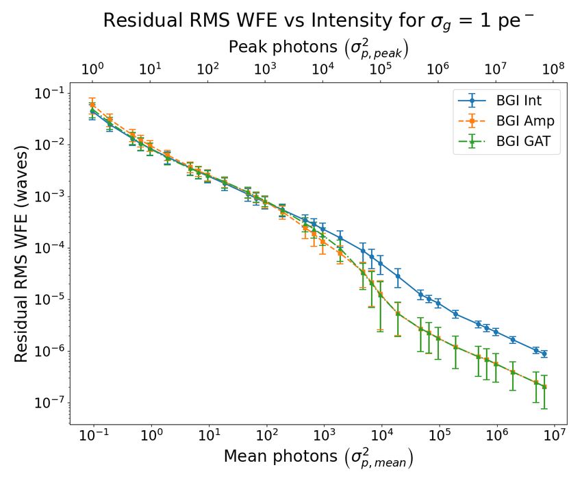
equivalent for the AEM, since the derivation for the bias and gain invariance for the IEM does not work for the
                AEM due to a square root. Thus, even though the AEM should have better performance than the IEM when
                Poisson noise dominates, we more often use the BGI IEM. Later in this paper, however, we will discuss a way
                to have a BGI form of the AEM, but it is more of a stepping stone to an even better error metric.
                    An issue of the IEM, however, is noise model mismatch. As mentioned previously, it has been shown that the
                IEM is the maximum likelihood estimate for an additive Gaussian noise model.4 Paxman et al. also derive an
                error metric for a pure Poisson noise case.4 However, in reality, the noise model is most accurately represented as
                a combination of signal-independent additive Gaussian noise and signal-dependent Poisson noise, which we will
                call mixed Poisson-Gaussian (PG) noise. Thus, because the IEM is maximum likelihood for additive Gaussian
                noise, but the true noise model is mixed PG noise, there is a noise model mismatch between the IEM and the
                noise in the data PSF. In previous work, we discussed how the generalized Anscombe transform (GAT) (shown
                in Eq. (4) later in this paper) can help with this noise model mismatch.5 This is because the GAT is a variance-
                stabilizing transform (VST) for mixed PG noise,6 which in short means that the variance for each pixel after
                the GAT is approximately the same, i.e., the variance is “stabilized.” In other words, the GAT transforms a
                mixed PG noise model to an approximately additive Gaussian noise model. Therefore, there should be a better
                noise model match between using the sum-squared error after performing the GAT on the simulated and data
                PSFs as the error metric compared to the IEM. We call this error metric of the sum-squared error between
                GAT-transformed simulated and data PSFs the GAT error metric (GEM). It also turns out that the square
                root function is a very simple VST that works well for Poisson noise at high intensity levels. This explains
                why the AEM may perform better than the IEM in some cases as mentioned before: when the noise model is
                more Poisson-like (i.e., high intensities), the AEM will out-perform the IEM, but when the noise model is more
                additive Gaussian-like (i.e., more dominated by read noise), then the IEM will out-perform the AEM. Note for
                the pure Poisson noise case, the GAT simplifies to the classical Anscombe transform, which has better variance-
                stabilization for pure Poisson noise than the simple square root function,7, 8 so the AEM could have been further
                improved by replacing the square root with the classical Anscombe transform for the pure Poisson noise model
                case, and it should have similar performance to using the Poisson error metric.4 However, once there is some
                additive Gaussian noise, we would expect the GEM to perform the best.
                   Since the GEM also has a square root function within it inside the GAT, the GEM has the same issue as the
                AEM in that the derivation of the bias and gain invariance that works for the IEM does not work for the GEM.
                However, in this paper, we developed a method that allows us to use the bias and gain terms derived for the
                BGI IEM case in service to the GEM and AEM, in effect creating BGI forms of the GEM and AEM. We then
                performed simulations to verify the validity of this method, and we demonstrate that the benefits of the GEM
                over the IEM and AEM as shown previously5 are maintained for the BGI GEM.

                                     2. INTENSITY, AMPLITUDE, AND GAT ERROR METRICS
                2.1 Intensity Error Metric
                The intensity error metric (IEM), EInt , is the normalized sum-squared error between the simulated and data
                PSFs, i.e.,                                       X
                                                                     w ◦ (I − D)2
                                                                                     x,y
                                                                          EInt =           X              ,                    (1)
                                                                                                 w ◦ D2
                                                                                           x,y

                where ◦ denotes a Hadamard product, w is a weighting function (such as a bad pixel mask), I is the simulated
                PSF, and D is the data PSF. This is a common error metric that is used in phase retrieval.1 The sum-
                squared difference in the IEM comes from its derivation of giving the maximum likelihood estimate for additive
                Gaussian noise model. While the true noise model is mixed Poisson-Gaussian, since the GAT (and the amplitude
                transform as well, though to a lesser extent) transforms the mixed PG noise model to an approximately additive
                Gaussian noise model, the GAT and amplitude error metrics will also contain a sum-squared difference but in
                the transformed space. Thus, the IEM, AEM, and GEM are similar to each other because they all contain a
                sum-squared difference.

                                                                        Proc. of SPIE Vol. 11443 1144348-2
Downloaded From: https://www.spiedigitallibrary.org/conference-proceedings-of-spie on 14 Jan 2021
Terms of Use: https://www.spiedigitallibrary.org/terms-of-use
2.2 Amplitude and GAT Error Metric
The amplitude error metric (AEM), EAmp , and GAT error metric (GEM), EGAT , can be thought of as performing
a transform on both the simulated and data PSFs before taking the normalized sum-squared error. The amplitude
transform is defined as (√
X for X > 0
A(X) = , (2)
0 otherwise
and accordingly the amplitude error metric is then
X
w ◦ [A(I) − A(D)]2
x,y
EAmp = X , (3)
w ◦ [A(D)]2
x,y
Similarly, the GAT error metric uses the generalized Anscombe transform (GAT), which is defined as
(q
X + 3/8 + σg2 for X + 3/8 + σg2 > 0
G(X) = , (4)
0 otherwise
and accordingly the GAT error metric is then
X
w ◦ [G(I) − G(D)]2
x,y
EGAT = X . (5)
w ◦ [G(D)]2
x,y
When σg = 0, the GAT simplifies to the classical Anscombe transform, which has better variance-stabilization
than the simple square root of the amplitude transform.7, 8
Note that the amplitude transform and GAT essentially clips negative values under the square root to 0.
While this prevents the problematic issue of dealing with complex values, this may introduces errors in cases
with negative numbers, which may be due to the bipolar Gaussian additive noise or negative bias. Thus, care
should be taken to ensure that not too many pixels are clipped when performing the transform. Another way to
deal with the clipped pixels is to mask them out with the weighting function, i.e., at the location of clipped pixels,
set wx,y = 0. This insures that the error metric is evaluated over the non-clipped pixels where no information is
lost, but it does sacrifice some information content of the data.
3. BIAS AND GAIN INVARIANT EXTENSION TO ERROR METRICS
Extending an error metric to be bias and gain invariant (BGI) typically involves replacing I with αI + β, where
α and β represent the gain and bias terms, respectively. Thus, the BGI forms of Eqs. (1), (3), and (5) are
X
w ◦ (αI + β − D)2
x,y
EBGIInt = X (6)
w ◦ D2
x,y
X
w ◦ [A(αI + β) − A(D)]2
x,y
EBGIAmp = X (7)
w ◦ [A(D)]2
x,y
X
w ◦ [G(αI + β) − G(D)]2
x,y
EBGIGAT = X , (8)
w ◦ [G(D)]2
x,y
Proc. of SPIE Vol. 11443 1144348-3
Downloaded From: https://www.spiedigitallibrary.org/conference-proceedings-of-spie on 14 Jan 2021
Terms of Use: https://www.spiedigitallibrary.org/terms-of-usefor the intensity, amplitude, and GAT error metrics, respectively. We have considered three methods to deal with
the bias and gain terms: 1) calibration is done to determine reasonable guesses for the bias and gain, and then
have α and β be fixed, 2) have α and β be unknown parameters, which are then solved for during optimization,
or 3) find analytic expressions that are functions of the simulated PSF that find reasonable estimates for α and
β, i.e., α and β become α(I) and β(I). These methods can be combined, such as doing a calibration in order
to have initial values when optimizing for α and β. Methods 2 and 3 have the advantage of not needing any
calibration, but between Method 2 and 3, it is not known whether Method 2 or Method 3 is guaranteed to be
better. For the work in this paper, we employ Method 3.
The analytic expressions used for α and β in Method 3 were initially done by Thurman1 and are explicitly
written in the appendix of Moore’s paper:9
h1i hD, Ii − hIi hDi
α= 2 (9)
h1i hI, Ii − hIi
hI, Ii hDi − hIi hD, Ii
β= 2 , (10)
h1i hI, Ii − hIi
where
X
hX, Y i = w◦X ◦Y (11)
x,y
X
hXi = w◦X (12)
x,y
X
h1i = w. (13)
x,y
These analytic expressions were derived for the IEM, where these values of α and β are such that ∂E/∂α =
∂E/∂β = 0. Using reverse-mode algorithmic differentiation (RMAD) to compute the gradient as proposed by
Jurling,10 and following his notation where X = ∂E/∂X: because α and β have the property that α = β = 0,
the gradient calculation when using the IEM is made simpler because there are no additional terms to I despite
α and β both having dependence on I due to chain rule of partial derivatives.9
A reasonable thought would be to do the same procedure (find α and β, then solve the system of equations
α = β = 0 to obtain analytic expressions for α and β) for AEM and GEM. However, the presence of the square
root in both the amplitude transform, Eq. (2), and GAT, Eq. (4), makes solving the system of equations for α
and β very complicated. Nevertheless, we have these expressions for α and β from the IEM in Eqs. (9) and (10),
so one may ask why not use them for AEM and GEM since they still provide reasonable estimates for α and β.
While this approach will work, and it will end up being the approach taken in this paper, special care needs to be
taken into account for the gradient calculation. For the AEM and GEM cases, using the expressions in Eqs. (9)
and (10) for α and β no longer guarantees that α = β = 0, so I will have additional gradient contributions
from the I dependence in both α and β. The derivation for these additional gradient terms is described in
Appendix A, and the full I gradient for all three metrics is described in Appendix B.
4. SIMULATIONS
To generate a simulated PSF, I, we had a circular exit pupil with a diameter of 128 pixels, and a wavefront was
generated over the exit pupil that was the linear superposition of Zernike polynomials up to 6th radial order,
ignoring piston (27 total polynomials). The Zernike coefficients were weighted such that the higher Zernike
terms had lower magnitudes than lower Zernike terms, and then the wavefront was scaled to have an RMS
wavefront error of 0.1 waves. The simulated PSFs were computed to be at 4 waves of defocus, so a quadratic
phase corresponding to 4 waves of defocus was added to the wavefront. The wavefront was zero-padded to have
an FFT size of 512 pixels before calculated the PSF as the squared magnitude of the Fourier transform of the
exit pupil. Then the center 256 pixel square of the PSF was used as the simulated PSF to reduce the effect of
Proc. of SPIE Vol. 11443 1144348-4
Downloaded From: https://www.spiedigitallibrary.org/conference-proceedings-of-spie on 14 Jan 2021
Terms of Use: https://www.spiedigitallibrary.org/terms-of-usealiasing. In terms of pupil and image sampling ratios, QP and QI , respectively, as defined by Jurling,11 QP = 4
and QI = 2.
To generate a noisy data PSF, D, with mixed PG noise, the simulated PSF was scaled to some amount
2
of peak photons, σp,peak before adding Poisson noise, and then Gaussian noise with standard deviation σg was
2
added. Then σp,peak and σg were changed to vary the amounts of Poisson and Gaussian noise. To have a slightly
better measure of the amount of Poisson noise in the data PSF, the mean intensity of the simulated PSF after
scaling for peak photons but before adding Poisson noise was calculated. The mean intensity corresponds to
2
σp,mean , and the average amount of Poisson noise in the data PSF is equal to σp,mean .
To test the accuracy of an error metric for a specific amount of mixed PG noise, 10 wavefronts were generated,
and for each wavefront, 100 noise realizations in D were generated. Then for each D, phase retrieval was
performed with that error metric starting from the true Zernike coefficients (ignoring piston), and then accuracy
was measured by the RMS difference between the true and retrieved wavefronts, also known as the residual RMS
wavefront error (WFE). We start from the true solution because we are testing accuracy, so this method allows
us to evaluate how much the retrieved wavefront deviates from the true solution for each error metric without
having to worry about issues of stagnation in local minima. The average and standard deviation of the accuracy
was found across all wavefronts and noise realizations, and the average σp,mean was found across the different
wavefronts. This was done for all three BGI error metrics, with the wavefronts and noise realizations being the
same across all error metrics.
To test the accuracy across various amounts of Poisson and Gaussian noise, σg would be fixed, and peak
2
photons σp,peak varied from 1 to 70 million photons. This was done for σg = 0, 1, 5 and 20 photo-electrons. The
accuracy of each error metric was found for each combination of Poisson and Gaussian noise.
5. RESULTS
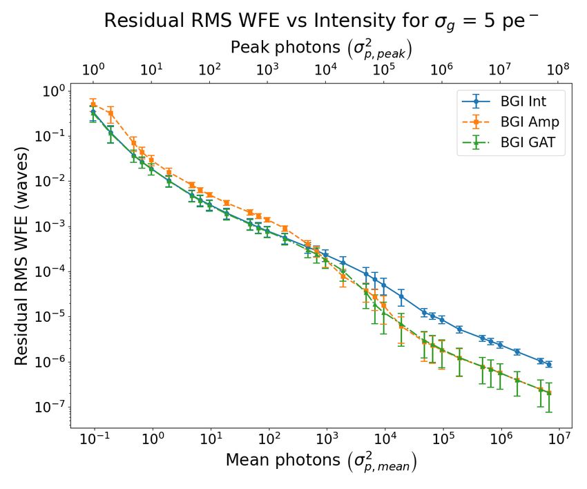
Figure 1 shows the residual RMS WFE as a function of different amounts of Poisson-Gaussian noise for each of
the three BGI error metrics. Lower residual RMS WFE is better and indicates higher retrieval accuracy. Subplots
(a), (b), (c), and (d) correspond to σg = 0, 1, 5, and 20 photo-electrons, respectively. The bottom horizontal axis
2
corresponds to mean photons of the true PSF, σp,mean , and the top horizontal axis corresponds to peak photons
2
of the true PSF, σp,peak , and these axes are also equal to the variances of the average and peak amount of Poisson
noise, respectively, in the data PSF. Note that σg = 0 is equivalent to pure Poisson noise. Moving from left to
right within a plot, the noise model moves from more Gaussian-like to more Poisson-like (except for σg = 0).
In subplot (d), the two large error bars for the BGI Amp error metric at low mean intensity indicate that the
retrieval accuracy was very inconsistent, and thus it should be interpreted that BGI Amp performs much more
poorly at those points than the mean accuracy might indicate.
6. DISCUSSION
In general, as the mean intensity increases, the residual RMS WFE decreases, regardless of error metric. This is
expected because as mean intensity increases, the signal-to-noise ratio increases, improving retrieval accuracy.
We expected that the IEM would perform better when the noise model is more Gaussian, the AEM to perform
better when the noise model is more Poisson. Since the noise model goes from more Gaussian to more Poisson as
mean intensity increases, we expected the IEM to perform better at lower intensities, and for AEM to perform
better at higher intensities, which we see in Figure 1. Thus, there is a cross-over point in each of the plots from
which IEM performs better to AEM performs better. In practice, it is difficult to know this point ahead of time,
as it is a function of the ratio between the amount of Poisson noise and Gaussian noise, the specific wavefront
under test, and system parameters (e.g., QP , QI , amount of defocus).
Because the GAT simplifies to the classical Anscombe transform when σg = 0, which has better variance-
stabilization for pure Poisson noise than the simple square root of the amplitude transform, we expected the
GEM to perform better than the AEM even for the pure Poisson noise case, which we seen for the lower levels
of mean photons in Fig. 1(a). At the higher levels of mean photons, the added term 3/8 in Eq. (4) is too small
to make a difference.
Proc. of SPIE Vol. 11443 1144348-5
Downloaded From: https://www.spiedigitallibrary.org/conference-proceedings-of-spie on 14 Jan 2021
Terms of Use: https://www.spiedigitallibrary.org/terms-of-use(a) (b)
(c) (d)
Figure 1. Residual RMS WFE vs various amounts of mixed Poisson-Gaussian noise for the different BGI error metrics.
Subplots (a), (b), (c), and (d) correspond to σg = 0, 1, 5, and 20 photo-electrons, respectively. The bottom horizontal
2 2
axis corresponds to the mean photons, σp,mean , and the top horizontal axis corresponds to the peak photons, σp,peak , for
two different estimates of the amount of Poisson noise in the data PSF. Lower residual RMS WFE is better and indicates
higher retrieval accuracy.
We expected the GEM to perform well for various mixed PG noise models, and Figure 1 shows this. In
general, the GEM performs comparable to or better than the IEM and AEM for all values of mixed PG noise.
Therefore, while for certain cases the IEM or AEM may perform slightly better than the GEM, the GEM is a
good general-use error metric that has comparable or better performance over all mixed PG noise cases.
Figures 1(a) and 1(b) do show that the IEM may perform better than the GEM for very low amounts of
Poisson noise when the Gaussian noise is low as well. This is likely due to the fact that the GAT has poor
variance-stabilization at very low intensities.8 However, interestingly, as the amount of Gaussian noise increases,
the variance stabilization of the GAT improves for low Poisson noise, which is why the GEM starts to perform
better than the IEM as seen in Fig. 1(c), and this improvement is more apparent in Fig. 1(d).
Future work involves comparing these results to Method 2 mentioned in Section 3, where α and β are
Proc. of SPIE Vol. 11443 1144348-6
Downloaded From: https://www.spiedigitallibrary.org/conference-proceedings-of-spie on 14 Jan 2021
Terms of Use: https://www.spiedigitallibrary.org/terms-of-useoptimization parameters; including analysis for a BGI form of an error metric that assumes pure Poisson noise;4
comparing convergence speed and convergence success rate of the different error metrics; and exploring whether
going between the different metrics is advantageous.
ACKNOWLEDGMENTS
We would like to thank Alden Jurling, NASA, for bringing to our attention the additional I gradient terms, as
well as allowing use of his python package WFSCore, which greatly simplified the phase retrieval process.
Funding: NASA Goddard Space Flight Center (GSFC) grant 80NSSC19K0650
APPENDIX A. GRADIENT CONTRIBUTIONS FROM BIAS AND GAIN
The gradient contributions to I from gain, α, and bias, β, denoted as I α and I β , respectively, were determined
through RMAD as described in Ref. 10. Starting from Eqs. (9) and (10), using quotient rule for derivatives, and
then simplifying, we obtain
− h1i w ◦ [αI + β − D] + α [I − µ(I, 1)]
Iα = 2 α (A.1)
h1i hI, Ii − hIi
hIi w ◦ 2 [αI + β − D] + [D − µ(D, I)]
Iβ = 2 β, (A.2)
h1i hI, Ii − hIi
where µ(X, Y ) = hX, Y i / hY i, which may be interpreted as the weighted average of X with weighting Y .
Note that the expressions for I α and I β are the same for all three error metrics, but α and β will be different
across error metrics, as seen by Eqs. (B.4), (B.9), and (B.14) for α and Eqs. (B.5), (B.10), and (B.15) for β in
the next section.
APPENDIX B. GRADIENTS FOR BGI IEM, AEM, AND GEM
The gradient expressions using RMAD for BGI IEM, AEM, and GEM only differ up to I, beyond which the
gradient expressions are the same and can be found in Ref. 9. It should also be noted that for AEM and GEM,
these gradients expressions are for pixels that are not clipped by the transform as discussed in Section 2.2. For
pixels that are clipped by the transform, the gradient for that pixel is zero. For the following gradient expressions,
Nc is the normalization constant for the error metric, α and β are calculated according to Eqs. (9) and (10),
respectively, I E is the gradient contribution to I from the error metric, and I α and I β are found according to
Eqs. (A.1) and (A.2), respectively.
B.1 Gradient for BGI Intensity Error Metric
Starting with Eq. (6):
X
Nc = w ◦ D2 (B.1)
x,y
1 X
EBGIInt = w ◦ (αI + β − D)2 (B.2)
Nc x,y
E=1
2
IE = αw ◦ (αI + β − D) E (B.3)
Nc
" #
2 X
α= w ◦ (αI + β − D) ◦ I E = 0 (B.4)
Nc x,y
" #
2 X
β= w ◦ (αI + β − D) E = 0 (B.5)
Nc x,y
Proc. of SPIE Vol. 11443 1144348-7
Downloaded From: https://www.spiedigitallibrary.org/conference-proceedings-of-spie on 14 Jan 2021
Terms of Use: https://www.spiedigitallibrary.org/terms-of-useI = IE + Iα + Iβ = IE .
Note that for the IEM, α and β are such that α = β = 0, which causes I α = I β = 0. This is not the case for the
BGI AEM and GEM.
B.2 Gradient for BGI Amplitude Error Metric
Starting with Eq. (7):
X
Nc = w ◦ [A(D)]2 (B.6)
x,y
1 X
EBGIAmp = w ◦ [A(αI + β) − A(D)]2 (B.7)
Nc x,y
E=1
1 A(D)
IE = αw ◦ 1 − E (B.8)
Nc A(αI + β)
!
1 X A(D)
α= w◦I ◦ 1− E (B.9)
Nc x,y
A(αI + β)
!
1 X A(D)
β= w◦ 1− E (B.10)
Nc x,y
A(αI + β)
I = IE + Iα + Iβ ,
where A(X) is defined by Eq. (2).
B.3 Gradient for BGI GAT Error Metric
Starting with Eq. (8):
X
Nc = w ◦ [G(D)]2 (B.11)
x,y
1 X
EBGIGAT = w ◦ [G(αI + β) − G(D)]2 (B.12)
Nc x,y
E=1
1 G(D)
IE = αw ◦ 1 − E (B.13)
Nc G(αI + β)
!
1 X G(D)
α= w◦I ◦ 1− E (B.14)
Nc x,y
G(αI + β)
!
1 X G(D)
β= w◦ 1− E (B.15)
Nc x,y
G(αI + β)
I = IE + Iα + Iβ ,
where G(X) is defined by Eq. (4). Note that the gradient expressions for BGI GAT look exactly the same as for
BGI Amp, only replacing the amplitude transform with the GAT.
Proc. of SPIE Vol. 11443 1144348-8
Downloaded From: https://www.spiedigitallibrary.org/conference-proceedings-of-spie on 14 Jan 2021
Terms of Use: https://www.spiedigitallibrary.org/terms-of-useREFERENCES
1. Thurman, S. T. and Fienup, J. R., “Phase retrieval with signal bias,” J. Opt. Soc. Am. A 26, 1008 (2009).
2. Fienup, J. R., “Phase retrieval algorithms: a comparison,” Appl. Opt. 21, 2758 (1982).
3. Fienup, J. R., “Phase-retrieval algorithms for a complicated optical system,” Appl. Opt. 32, 1737 (1993).
4. Paxman, R. G., Schulz, T. J., and Fienup, J. R., “Joint estimation of object and aberrations by using phase
diversity,” J. Opt. Soc. Am. A 9, 1072 (1992).
5. Tang, J. S. and Fienup, J. R., “Improving accuracy of phase retrieval with mixed Poisson-Gaussian noise
using the generalized Anscombe transform,” in Imaging and Applied Optics Congress , OSA Technical Digest
(Opt. Soc. Am.), paper CF2C.4 (2020).
6. Starck, J.-L., Murtagh, F., and Bijaoui, A., Image Processing and Data Analysis , Cambridge University
Press (1998).
7. Anscombe, F. J., “The transformation of Poisson, binomial and negative-binomial data,” Biometrika 35,
246 (1948).
8. Yu, G., “Variance stabilizing transformations of Poisson, binomial and negative binomial distributions,”
Statistics and Probability Letters 79, 1621 (2009).
9. Moore, D. B. and Fienup, J. R., “Ptychography for optical metrology with limited translation knowledge,”
Appl. Opt. 55, 4596 (2016).
10. Jurling, A. S. and Fienup, J. R., “Applications of algorithmic differentiation to phase retrieval algorithms,”
J. Opt. Soc. of Am. A 31, 1348 (2014).
11. Jurling, A. S., Bergkoetter, M. D., and Fienup, J. R., “Techniques for arbitrary sampling in two-dimensional
Fourier transforms,” J. Opt. Soc. of Am. A 35, 1784 (2018).
Proc. of SPIE Vol. 11443 1144348-9
Downloaded From: https://www.spiedigitallibrary.org/conference-proceedings-of-spie on 14 Jan 2021
Terms of Use: https://www.spiedigitallibrary.org/terms-of-useYou can also read