PROPERTIES OF STARS Lezione III-Fisica delle Galassie Laura Magrini - Capitolo 3 di Binney & Merrifield (1998)

PROPERTIES OF STARS
 Lezione III- Fisica delle Galassie

 Capitolo 3 di Binney & Merrifield (1998)
Lezione 4 di M. Pettini (https://www.ast.cam.ac.uk/~pettini/STARS/).
 Cap. ‘Binary Systems and Stellar Parameters’
 Carrol & Ostlie

 Laura Magrini

Aim of this lecture
■ Derive the main physical properties of stars from observations:

o Mass
o Radius
o Age
o Chemical composition (in the next lectures)

à Many physical relations involves these quantities
à They are often only theoretically determined

à Need strong observational constraints

The masses of stars
 The most important property of a star is its mass.

à It determines the lifetime in the main sequence
à It determines the final evolution
à It can can measured ONLY studying the gravitational interaction with other objects
à It can be measured in Binary (or Multiple) Systems

We consider here only binary systems, dividing them in:
■ Visual binaries
■ Eclipsing binaries
■ Spectroscopic binaries

How many binary stars?
 • More binaries in the youngest systems
 • Following the model of Stahler &
 Sadavoy (2017) all stars were born at
 least in binary system
 • Even the Sun had a companion, named
 Nemesis

 A radio image of a triple star system forming within a
 dusty disk in the Perseus molecular cloud obtained by
 ALMA in Chile.
 (Image: Bill Saxton, ALMA (ESO/NAOJ/NRAO), NRAO/AUI/NSF)

 • Their presence has an effect on the
 Colour-Magnitude diagram
 • Separate sequence for binary and
 single stars

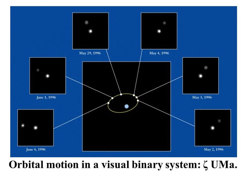
Binary systems: Visual binaries
 Stellar masses can be measured only in binary systems where we can estimate the effect of
 gravitational forces.

 There are about 1000 close-binary systems, in which both components are visible.
 • Detached à no interactions (material flowing from a star to the other)
 • Strong bias towards the more common stars: low-mass stars
 • Short or medium periods: observational bias again!

Binary systems: Visual binaries
1. Both stars are visible: systems relatively close to us so that the individual stars can be resolved
Visual Binary: their orbits can be studied à by monitoring them over the years
 • Observations repeated in time to derive orbital parameters
 • To separate parallax, proper motion and orbit effects

Binary systems: Visual binaries
 • Separate parallax, proper motion and orbit effects

 Single star

 Binary system of stars

 Triple system of stars

Binary systems: Visual binaries
Face-on systems: Face-on system

The distance from the centre of mass is inversely
proportional to the mass of the stars:

 m1 r1= m2 r2

We can measure the angular distances from the
 In this example m1=2 m2
centre of mass:

 From the general 3rd Kepler law we can derive
 1=r1/d also the total mass (where = 1 + 2):
 2=r2/d

Where d is the linear distance to the system.

 And having the mass ratio, we can have the
Thus the ratio between the angular distances of the masses of the two components
two stars is à We must also know the distance d to the
 m1/m2= 2/ 1 binary system
proportional to the mass ratio.

Binary systems: Visual binaries

From the ideal face-on case, to real observations….

To derive the masses from the angular distance measurements 1 and 2, we need:

i) Measure the parallax of the systemà they are usually close systems, thus their
 parallax can be measured à we need to observe the system for more than one year

ii) Measure the proper motion of the centre of mass à find the point of the system that
 move at constant velocity

iii) Derive the inclination of the plane of the orbit relative to the plane of the sky à it
 isn’t easy!

Binary systems: Visual binaries
 Consider the special case where the orbital plane
Line of Nodes:
intersection between is inclined at angle i to the plane of the sky.
the plane of the orbit
and the sky
 Reality is more complex, and orbit are often inclined
 along both the major and minor axes!

 If the system is inclined (angle i), the mass ratio
 does not change
 1’= 1 cos i
 2’= 2 cos i

 Thus the ratio between the angular distances of
 the two stars is:

 m1/m2= 2’/ 1’

 but it affects the estimation of the total mass, in
 which the uncertainty on the determination of
 the cosine remains.

Binary systems: Visual binaries
 To evaluate the sum of the masses properly à measure the inclination angle i

 • Estimate the differences in the location of the focus of the observed ellipse and the centre of mass
 (located at the position of the projection of the ‘true’ focus on the plane of the sky)

 • The real situation is even more complicated because in general the orbital plane is inclined along the
 minor and major axes!

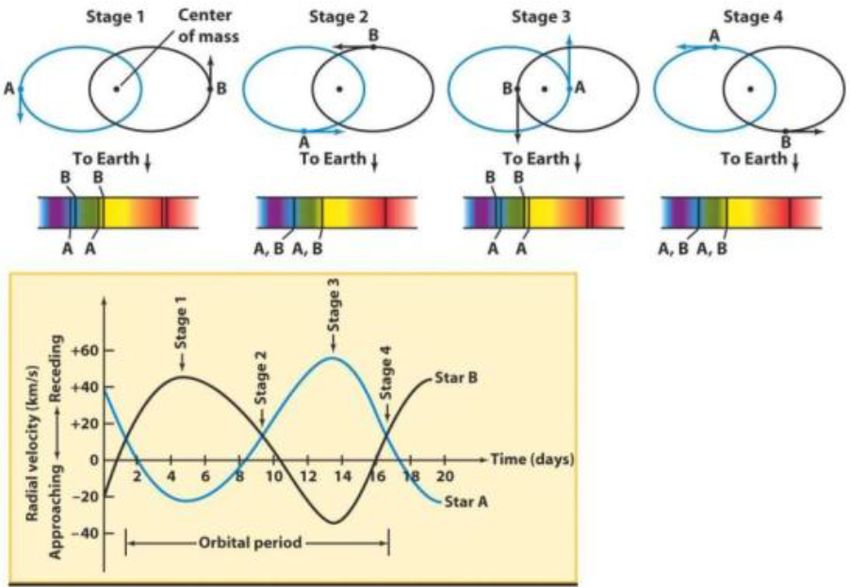
Binary systems: Spectroscopic binaries
2. The stars cannot be separated (more distant objects or more close orbits)
• the spectrum of the system is seen as the superposition of two set of spectral features (different
 if stars have different spectral type)à double-lined spectroscopic binaries
• their orbital motions are seen as Doppler shifts in their spectra.

Binary systems: Spectroscopic binaries
• The radial velocity component (to Earth) modify periodically the composite spectra of the
 system
• Need repeated observations

The maximum blueshift and redshift we measure within an orbit are lower limits to the true
velocities because of the unknown inclination i of the orbital plane to the line of sight:

 v1 rmax = v1 sin i and v2 rmax = v2 sin i.

 i=900

 V sin i

 Observer
 V

Binary systems: Spectroscopic binaries
Considering that spectroscopic binary are close systems, they tend to have circular orbits
(tidal forces) and their velocities can be expressed as:

• v1= 2 a1/P and v2= 2 a2/P à at small eccentricities e

The units of stellar mass
Stellar masses are measured in units of Solar mass
• Considering that the mass of the Sun
 is much larger than the Earth mass, we have:

 G M⊙ P⊕2=4 2 a ⊕ 3
 where P⊕ is the period of revolution (1 year), a is the mean distance Earth-Sun (1
 AU).

• Taking the ratio between the general equation and that for the Earth-Sun system
 (m1 + m2) P2 = a3

 So, if periods are expressed in years and distances in AU, star masses will be in
 Solar masses à we usually derive the total mass of the system

 M ⊙=1.99 X 1033 kg [the mass of the Sun is computed in the same way, considering the
 system Earth/Moon]

Binary systems: Eclipsing binaries
2. The stars cannot be separated
 • Eclipsing Binary: the total brightness drops when they periodically eclipse each other.
 • There is no ambiguity about the orientation of the orbit (the orbit on the same plane,
 edge-on, i=90o or close to it) à note that for i > 75o, sin(i) > 0.9, so the error in the masses,
 assuming i=90o is only 10%!

Binary systems: Stellar radii
We can both measure the mass of the system, and, moreover, the radii of the two stars.
When the eclipse is total, we can deduce the radii of both stars from accurate timing of the phases of the
eclipse.
With the assumption the the secondary stars is moving perpendicularly to our line-of-sight during the
eclipse, the radius can be derived:

 Secondary star

 Primary star

Where ta and tb are the times of the first contact and
minimum light, respectively, and v=va+vb is the relative
velocity of the two stars

Binary systems: effective temperatures
The ratio of the effective temperatures of two stars in an eclipsing system can be estimated assuming
that they are Black Bodies, and measuring the among of light received during the eclipse.

 Fr= σ T4 à radiative surface flux
 When both stars are visible:

 Frl and Frs are the radiative flux of the primary and secondary
 stars.
 Primary minimum: when the hotter star (in this case the
 smallest one) pass behind the primary companion.

 Secondary minimum: when the hotter star (in this case the
 smallest one) pass behind the primary companion.

Binary systems: effective temperatures

What we usually measure are magnitudes, so for instance, if the maximum magnitude (both stars
visible) is m0=6.3, and mprim_min=9.6, and msec_min=6.6, we can derive:

(m=2.5 log L à L= 10 (2 m/5)=100 m/5.....)

And thus, we can find the ratios between the radiative fluxes and the temperatures.

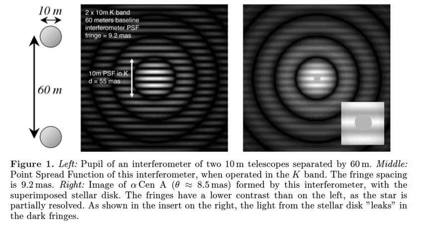
Interferometry: Stellar radii
• INTERFEROMETRY for nearby stars
Long baseline interferometers now measure the angular diameters of nearby stars with sub-percent
accuracy.

The finite angular size of a star (in Figure α-Cen A with an angular diameter of 8.5 mas) causes a
reduction of the contrast of the fringes, that can be measured with great accuracy.
There is a direct relation between the visibility of the fringes and the angular size of the star
(Zernike-Van Cittert theorem), that allows to retrieve the angular size of the star.
Telescope diameter Unresolved star Alpha Cen A d=8.5 mas
 Separation between telescopes

Lunar occultation: Stellar radii
• LUNAR OCCULTATIONS

The angular velocity of the Moon is 0”.52/s.
A star similar to the Sun, at 10 pc, has d= 0.00038”.

t=0.00038”/0.52”s-1 =0.0007 s

à We need to measure very short time intervals!
The occultation pattern varies:
• for dwarf is diffraction limited
• giant stars has a smooth profile

From the Stefan-Boltzmann law: Stellar radii
Stefan-Boltzmann Law gives us the energy radiated per sec per unit area on the surface of a
blackbody

 E = σ T4
where σ is a constant, σ = 5.67 10-5 erg s-1 cm-2 K-4

The total amount of energy radiated per second by a star (the luminosity) can be found by
multiplying E in the equation above by the total surface area of the star.
For a sphere, the area is 4πR2, where R is the radius of the star.

 L = (4 R2) σT4
We can also find the temperature using Wien’s law or from spectroscopy.
Therefore, we can then find the radius using

 R = √L/4 σT4

* Here we assume that the star is Black Body

From the Stefan-Boltzmann law: an example
Stellar radii are usually given in Solar units:
From the S-B law, we have
 L/L⦿ = (4 σR2T4)/(4 σR⦿T⦿4) = (R/R⦿)2(T/T⦿)4

 R/R ⦿ = (T ⦿ /T)2(L/L ⦿)1/2

To find the ratio L/L ⦿, we use the absolute magnitudes of the stars.
The magnitude scale is a logarithmic scale. For every decrease in brightness of 1 magnitude, the star
is 2.51 times as bright. Therefore, L/L ⦿ can be found from the equation

 L/L ⦿ = 2.51Δm
where Δm = m ⦿ - m

Sirius has a visual magnitude of -1.44 and a parallax of p=379.21 mas. From the parallax, we
estimate distance:
 d = 1/p = 1/0”.37921 = 2.63 pc

The absolute magnitude is:

 M = m - 5 log d + 5 = -1.44 - 5 log (2.63) + 5 = 1.46

The Sun has an absolute magnitude of 4.83, a temperature ~5800K and the temperature of Sirius is
~9500K.
 R/R ⦿ = (5800/9500)2(2.513.37)1/2 = 1.76

Comparing observations with theory:
 stellar radii in and out the main sequence
 Empirical stellar radii in the HR diagram

 Giant stars
Luminosity

 Dwarf stars

Comparing observations with theory:
 The mass-luminosity relationship

When we bring together the best determinations of stellar masses from different types of
binary stars, we find a well defined mass-luminosity relation for hydrogen burning dwarf
 • Theories of stellar evolution must be able to
stars: reproduce such a relationship

 • The location in the plane is determined only by
 the mass

 • Stars do not evolve along the main sequence,
 they evolve off the main sequence.

 Torres et al. 2010

 • If L ∝ dM/dT then T ∝ M/L = M-2.5
 the steep slope of the stellar mass luminosity
 relation implies a very strong dependence of the
 stellar lifetimes on their mass

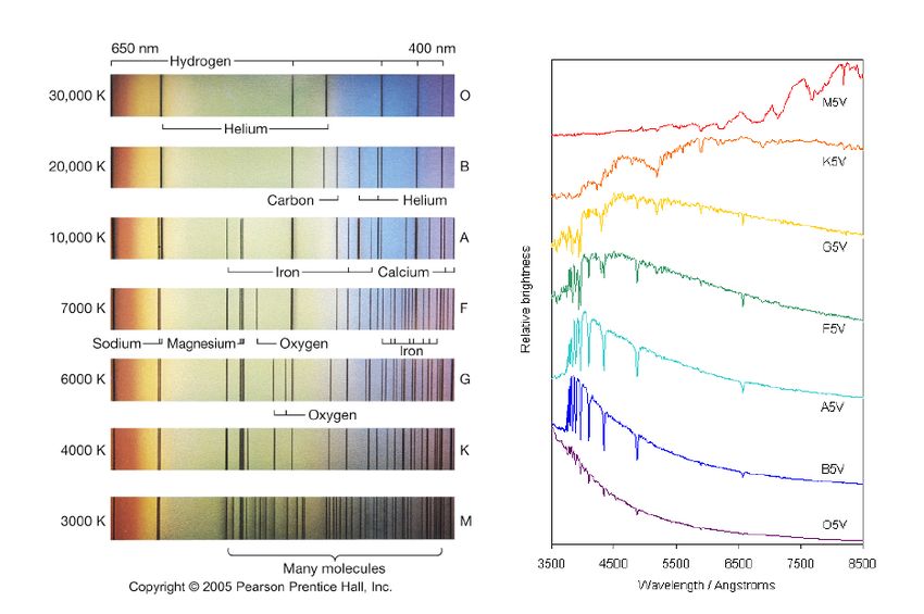
The spectral classification of stars
We have seen how the main parameters (mass and radius) can be measured, now we want
to infer other quantities form the spectral appearance of stars:

■ Stars are classified via their spectra

■ The classical classification schema:

 O B A F G M [R N S]

Based on the observed variation of ratios of line strengths of successive ionization stages
of chemical elements has then been recognized to be primarily a temperature sequence.

The spectral classification of stars

The spectral classification of stars
Each class is subdivided into 10 sub-classes, with Teff decreasing from sub-class 0 to 9. Thus
we have spectral classes O9 and B0, the former being just hotter than the latter.

 O and B à `early-type’
 K and M à `late-type'.

The spectral classification of stars
The meaning of the spectral sub-classes (luminosity classes):

Antonia Maury noticed difference between stars with the same temperature but with different
luminosity, call c-characteristic.

If we consider stars of the same Teff but different luminosity, we have, from the Stefan-Boltzmann law,
that the star should have a different radius.

 L=4 σ R2Teff4

For instance, the surface density and gravity are lower in stars of larger radii.

As a consequence, stars with different luminosities (at a given Teff) will have different conditions in their
photospheres and their spectra will contain different absorption lines.

 Thus, the absorption line widths provide a measure of the `Luminosity Class'.
 A0

 AV

The spectral classification of stars
 Luminosity classes are indicated
 by roman numerals, from I to V
 in order of decreasing
 luminosity.

 • Class I: supergiants
 • Class II: bright giants
 • Class III: giants
 • ClassIV: subgiants
 • ClassV: main sequence,
 sometimes referred as
 `dwarfs'.
Sun G2V B-V=+0.63 Teff=5777

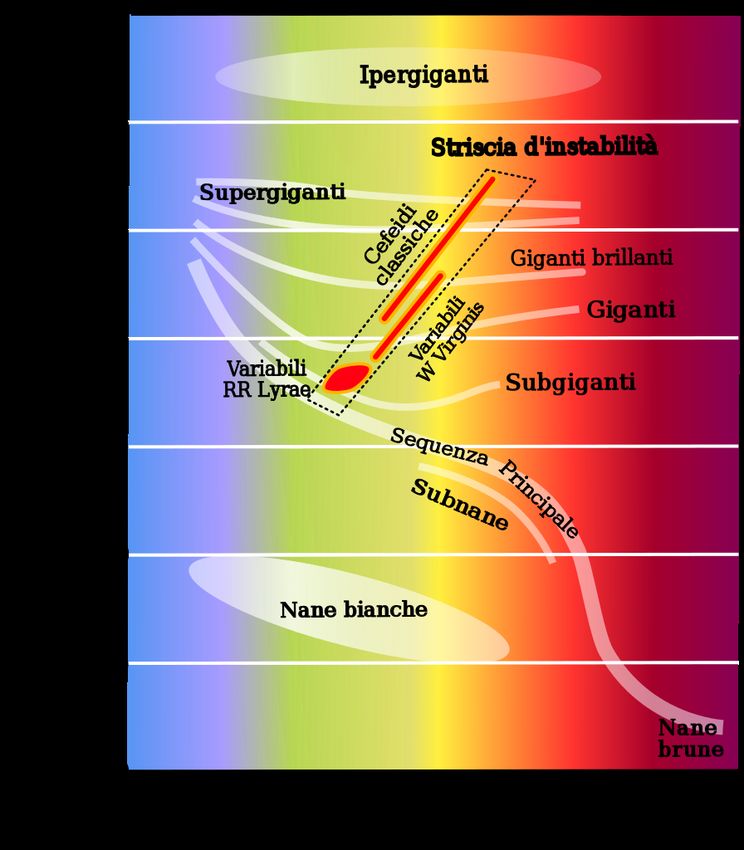
The classification of stars: variability

 Stars outside the standard
 classification system:

 • Cepheids
 • RR Lyrae
 • Variable stars

The classification of stars: variability

The HR diagram: classification based on the evolutionary
phase
 • MS: phase of burning hydrogen in
 cores
 P-AGB AGB • MSTO (turn-off): end of the MS
 BS phase.
 • SGB (sub-giant branch): H burning in
 shell, with increasing brightness
 • RGB (red giant brach): the star burns
 He, and loses mass and eventually
 SBG
 becomes a horizontal branch (HB) star.
 • AGB (asymptotic giant branch): after
 the He fusion in its core, energy comes
 from He fusion in a shell around the inert
 WD
 carbon-oxygen core
 • P-AGB (Post-AGB): towards the WD
 phase
 • Blue stragglers (BS) affected by close
 encounters in the dense cluster region
 • WD (white dwarf): no nuclear reaction

The HR diagram: classification based on the evolutionary
phase

• This classification is related to stellar evolution.
• Here an example of the evolution of a low- and intermediate mass stars in the HR
 diagram
• In a cluster (group of coeval stars) the presence of stars in some evolutionary stages
 is indicative of the cluster age.

From the HR diagram: information on the stellar age

 HR diagrams of star clusters
 (coeval and chemically
 homogeneous group of
 stars) allows us to analyze
 evolutionary effects.

 This image shows a combined HRD for 32 open clusters made with the second Gaia
 data release data.
 Colour indicates cluster age: stars that are members of younger clusters are shown in
 blue, stars belonging to older clusters - in red. The effects of cluster age can clearly be
 distinguished (T ∝ M-2.5, older cluster less massive MS-TO stars…)

Ages of stars
For stars that do no belong to star clusters, measuring ages is much more difficult.
A stellar population is a mixture of stars with different ages, stars in particular evolutionary phases can
give indication of the age of the population.

Ages of stars: Isochrone fitting
An isochrone is a curve on the CMD (or in the HR diagram) which defines the location of all stars of a
given age.
 The isochrone fitting technique allows to estimate the cluster ages
 Limits: rely on the assumptions of the stellar models, age can varies from isochrones to isochrones, …

Ages of stars: Isochrone fitting
• Isochronal Ages for field stars:

 o Compare a luminosity and color of a star to a grid of theoretical stellar models calibrated
 against empirical observations of globular and open clusters.
 o Gaia’s precise distances and photometry expands the volume isochronal ages

 Limits:
 • Reliable results for the turn-off stage and the
 sub-giant branch

 • For other populations there may exist many
 age-values estimations for the same object
 due to the overlapping of the different
 isochrones.

 • Need to know metallicity

Errors from Unified tool to estimate Distances, Ages, and Masses (UniDAM) (Mints and
Hekker, 2017)

Ages of stars: Isochrone fitting
 Limits:
 • For giant stars: isochrones of different
 ages are over posed
 • In the zoomed plot: log(age) from 7.8
 to 10.2
 • Large errors in the derived ages

Grid of PARSEC isochrones at solar metallicity

Ages of stars:
 stellar properties related to age
Comparison with theoretical models is not always applicable.
We can search for stellar properties related to the age of the star.
These relationships need to be calibrated against ages derived in different ways.

• Magnetic activity
• Stellar structure
• Nuclear cosmochronology
• Chemical composition

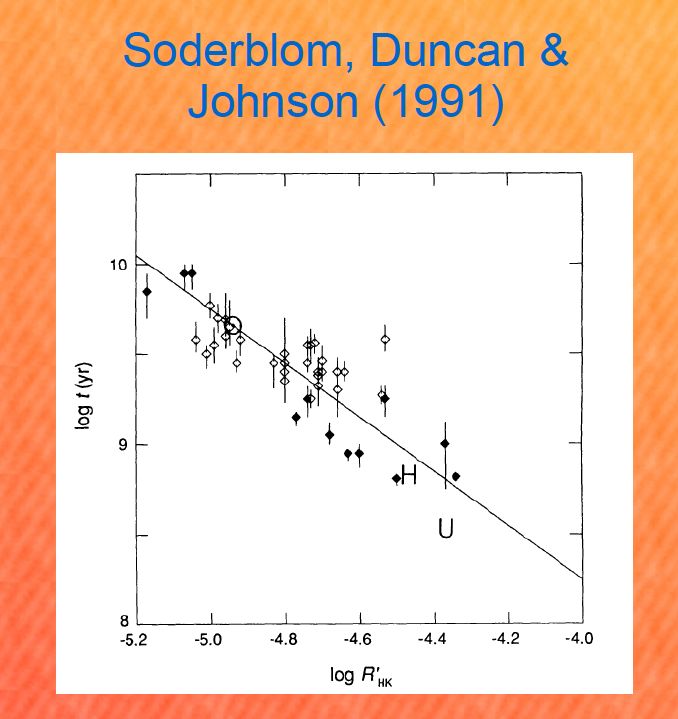
Ages of field stars:
 relationship with the magnetic field and rotational velocity

Magnetic fields play an important role in stellar evolution. It regulates stellar rotation from the early
stages of star formation until the ultimate stages of the life of a star.

‘Isolated’ stars slowly spin-down as their age increases, as observed by Skumanich (1972).
For G-type stars in the main-sequence (MS), the projected rotational velocity decreases with age

 v sin (i) ∝ t−1/2

The rotational braking is believed to be caused by stellar winds, which, outflowing along magnetic field
lines, are able to efficiently remove the angular momentum of the star.

Indicators of magnetic activity:
• surface spot coverage
• emission from the chromosphere, transition region or corona are closely linked to rotation

 See Vidotto et al. 2014

Ages of field stars: relationship with the magnetic field
• Gyrochronology:

 o Rotation, age, and magnetic field strength are tightly coupled for solar–type stars (fast rotators
 produce strong magnetic fields, giving rise to stellar winds that carry away angular
 momentum, reduce the interior rotational shear of the star, and thereby weaken its magnetic
 field)

 o Need to be calibrated with measurements of period of rotation in star clusters

 o Periods are measured estimating the variation of the magnitude due to rotation of the
 starspot.

 Limits:

 • The relationship saturates for
 fast rotators

 • Time consuming and precision
 photometry
 o
 • LSST (large Synoptic telescope)
 will improve and enlarge its
 applicability

Ages of field stars: relationship with the magnetic field
The rotational periods are longer for the older
populations Simulations for the LSST telescope
For a given population, they are longer for the
cooler (older) stars [on the left side]

 The photometric variation is very small, but still detectable

 mmag
 Period in days

Ages of field stars: relationship with the magnetic field
Age-activity relation:

 o Stellar flares, which trace the strength of the magnetic field of the star, are another
 photometric proxy for stellar age à activity decreases with increasing stellar age

 o Cluster observations will indicate how the frequency and intensity of stellar flares vary with
 stellar age and mass.

 Limits:
 • Can estimate ages
 for the youngest
 populations

 • Missing
 calibrations for the
 oldest populations

Ages of field stars: from stellar structure
Measuring the vibrational modes of stars, we can study the internal physical conditions and from them
to infer stellar chemical composition, rotation profiles and internal physical properties such as
temperatures and densities.

 A few examples of stellar vibration modes

Stellar oscillation can be measured only from the space.
There are several space missions aiming at: i) find planets, ii) measure stellar oscillations, as:
• CoRoT was a ESA space observatory mission which operated from 2006 to 2013,
• Kepler is a space observatory mission launched by NASA on 2009, which had a ‘second life’ as
 Kepler K2

• à They performed asteroseismology by measuring solar-like oscillation in stars.

In the next years: PLATO and TESS satellites

Ages of field stars: from stellar structure
Asteroseisomology
 o The oscillation frequencies of a star depend on the properties of stellar interior.

 o Since these are tightly linked with the mass and evolutionary status, the mass and age of a star
 can be estimated from the comparison of its oscillation spectrum with stellar model
 predictions.

 Limits:
 • Only for solar type and giant
 stars where convection is
 near to the surface

 • uncertainties due to
 chemical composition à
 need spectroscopy

 • Poor understanding of
 processes in stellar interiors

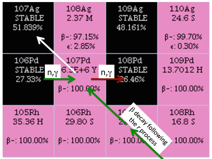
Ages of field stars
• Nuclear cosmochronology

 o High-precision method based on the spectroscopic abundances of heavy radioactive isotopes,
 taking into account the constant rate of radioactive decay, for example 238U and 232Th,
 compared to stable isotope.

 o Based on the knowledge about the half-life time for these elements, the age of the matter from
 which the star was created, can be estimated.

 Limits:
 • Scarce abundance of uranium
 and thorium lines in the stellar
 spectra

 • Poor knowledge of the initial
 isotopic ratios

Ages of field stars

• Chemical clocks [more details in the next lectures]:

As the time scales of the various nucleosynthetic processes are different, the chemical abundance ratio of
two elements produced by two different channels provides a time estimate.

 o [C/N] in giant stars: during the RGB phase the convection dredge-up material in the
 photosphere, changing the [C/N] abundance ratio. The change depends on the mass of the
 stars, and thus can trace its age.

 o [α/Fe] : α elements are synthesized in high-mass, very short-lived stars. Iron is produced by
 both SN II and type I supernovae (SN Ia), the latter with longer lifetimes >0.3 Gyr. Comparing
 their relative abundances provides a measure the age.

 o [Y/Mg]: Yttrium is produced by intermediate- and low-mass stars, while Mg by massive stars,
 on different timescales, making of this ratio another good proxy for stellar age dating.

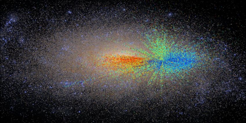
Map of the ages of the MW disc

Age distribution for a sample of red giant stars ranging from the galactic center to the
outskirts of the Milky Way, analyzed by Melissa Ness and colleagues. The sample is
embedded in a simulation of a Milky Way-like galaxy.
Age is color coded, with the youngest stars shown in blue, the oldest stars in red, and
middle-aged stars in green. The age distribution, including the obvious fact that the
oldest stars are concentrated closer to the galactic center, confirms current models of
galactic growth that have the Milky Way growing from the inside out.

How is the Milky Way composed? Which are the main stellar populations in the
different component of the Galaxy?

 The luminosity-weighted relative
 contribution of various evolutionary
 stages to the integrated bolometric
 luminosity of a simple stellar
 population as a function of age
 (Renzini & Buzzoni 1986) and their
 TO mass

 à directly linked to the age of the
 stellar population

Stellar population in the Milky Way

Classically the stellar populations of the Milky Way were divided in:
• PopI, younger and metal richer stars, located in the thin disc
• PopII, older, metal poorer, located in the thick disk and halo
 A modern classification is shown in the Table:

Stellar population in the Milky Way

 Characteristics of Pop I and Pop II stars

Halo:
 Globular clusters
 RR Lyrae
 Type II Cephedis Thick disk:
 12 < Age < 14 Gyr K M stars
 Miras
 RR Lyrae
 8 < Age < 14 Gyr
Bulge:
K M giants Thin disk:
RR Lyrae A M stars
A stars Subgiants
1 < Age < 14 Gyr Planetary Nebulae
 1< Age < 8 Gyr

 Spiral arms:
 O B stars (young and massive)
 Type I Cepheids
 Age < 0.1 Gyr

 Population I
 Population II
 Bulge Population(s)

The missing ingredient:
 population III stars

The first stars are a metal-free (massive) Population III stars formed after the Big Bang
• within a few hundred million years become supernovae and seed the interstellar
 space with sufficient heavy elements to produce Population II stars.

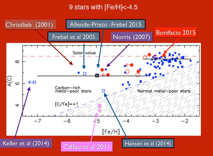
Low mass very metal poor stars open
new horizons:
■ Metal poor stars (first progenitors of possible PopIII stars) are usually
 enhanced in other elements, as C

■ They have sufficient global metallicity to allow their formation (with
 normal prescriptions…)

■ The Caffau star requires new mechanisms for low mass formation, e.g.,
 dust cooling or fragmentation

Summary
■ To calibrate models (stellar evolution, Galactic evolution, etc.) we need to have
 ‘direct’ measurement of basis ingredients:

■ Stellar masses à from gravitational forces in binary systems

■ Stellar radii à in eclipsing binaries (or interferometry, occultation)

Ø Stellar evolution models MUST much the empirical relationships found between:
 mass, radius, luminosity

§ Stellar ages à from isochrone fitting to chemical clocks, measuring the most
 difficult quantity in astrophysics

Ø With all this quantities in hand, we can map the properties of the stellar populations
 in our Galaxy (and beyond)

 à Missing piece of information: chemical composition and kinematics