QE-2021: Hands-on session - Day-2 - (Convergence-tests calculations) Anton Kokalj, Pietro Delugas, Paolo Giannozzi
←
→
Page content transcription
If your browser does not render page correctly, please read the page content below
QE-2021: Hands-on session – Day-2

          (Convergence-tests calculations)
         Anton Kokalj, Pietro Delugas, Paolo Giannozzi,
Matic Poberžnik, Cristiano Malica, Subrahmanyam Sappati, Lei Qiao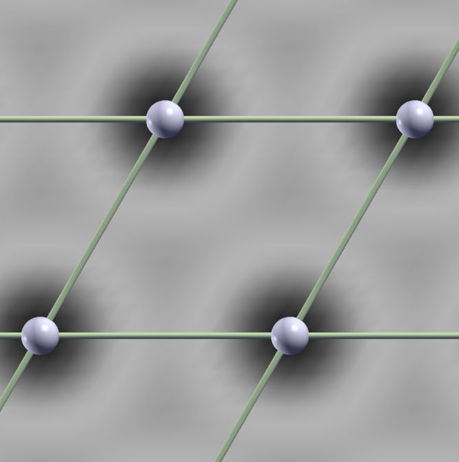
QE-2021: Hands-on session – Day-2

Topics of Day-2 hands-on session:

1. How to make basic convergence tests (example1.Si/)

2. How to deal with metals (example2.Al/)

3. How to deal with ultrasoft pseudopotentials and with spin polarization
   (example3.Fe/)

To get the latest version of the exercises, move to Day-2/ directory and execute:
     •   git pull
Beware: if you changed some input files in Day-1/ then git pull will fail and you
will need to do:
     •   git stash
     •   git pull
     •   git stash apply

QE-2021: MaX School on Advanced Materials and Molecular Modelling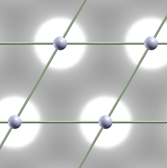
1. Bulk system: Silicon
Self-consistent calculation (and a series of tests) for Silicon in the diamond structure:

• move to Day-2/example1.Si/ directory

• look at the input file pw.si.scf.in. It is composed of three “namelists” &CONTROL
  (note that calculation = ’scf’ is the default value), &SYSTEM, &ELECTRONS,
  followed by three “cards” ATOMIC SPECIES, ATOMIC POSITIONS, K POINTS

• in the &CONTROL namelist notice the following two variables (they are commented):
    – outdir: temporary directory for large files. Must be writable, will be created if
      not existent. You may set environment variable ESPRESSO TMPDIR instead.
    – pseudo dir: directory where pseudopotential (PP) files are kept. It must exist,
      be readable, and contain the required PP file (in this example, Si.pz-vbc.UPF
      for Silicon). You may set environment variable ESPRESSO PSEUDO instead.

(note that for the hands-on exercises we rely on ESPRESSO TMPDIR and
ESPRESSO PSEUDO environmental variables, hence we don’t need to set outdir
and pseudo dir variables)

QE-2021: MaX School on Advanced Materials and Molecular Modelling    Example: Day-2/example1.Si/
Providing atomic structure in input
How is the crystal structure defined? This is a
very simple case: the diamond lattice is an fcc
(face-centered cubic) lattice with two atoms per
unit cell. You need to specify:
– What is the Bravais lattice?
ibrav=2, meaning fcc lattice
– How many and which parameters are needed to completely define Bravais lattice?
just one: celldm(1)=10.2, lattice parameter a in a.u.
– How many atoms there are in the unit cell?
nat=2: two atoms
– How many di↵erent atomic species are present?
ntyp=1: one species
– Which ones, described by which pseudopotential?
See card ATOMIC SPECIES
– Where the atoms are located in the unit cell?
See card ATOMIC POSITIONS: here, in Cartesian axes, in units of a (“alat”)
Notice that there are several alternative methods to specify an atomic structure!
QE-2021: MaX School on Advanced Materials and Molecular Modelling Example: Day-2/example1.Si/Brillouin zone (BZ) sampling
k-points are described in the K POINTS card. One has to choose
• Whether to provide a list of k-points or a uniform grid
• If a list is chosen: provide a list of k-points in the Irreducible BZ and corresponding
symmetry weights; the latter do not need to add up to 1, they are normalized by
the code
Frequently Asked Question: where do I find special k-points and their weights?
Answer: 1) in papers, 2) use an auxiliary code kpoints.x, 3) use uniform grids
• If a uniform grid is chosen: specify Monkhorst-Pack parameters (Phys. Rev. B 13,
5188 (1976)) and o↵sets along the three directions (uniform k-point grids are covered
in more detail in section 1.2 below).
QE-2021: MaX School on Advanced Materials and Molecular Modelling Example: Day-2/example1.Si/Running the pw.x code
For serial (single processor) execution you can use
• pw.x -in pw.si.scf.in > pw.si.scf.out
(note: input redirection pw.x < pw.si.scf.in works but it is not recommended on parallel machines)
Look at the directory specified by outdir (in our case $ESPRESSO TMPDIR) and its
content:
•ls $ESPRESSO TMPDIR
silicon.save silicon.xml
(to see only these files, you may need to use ls $ESPRESSO TMPDIR/silicon.*)
The directory contains a data directory (silicon.save/) with binary data files for
further processing and an XML file (silicon.xml) with general information on the
run. The name of the various files is determined by the value of the prefix variable
and by their content.
Do not run two instances of pw.x that access the same outdir with the same prefix!
Unpredictable behavior may follow (the directory is used for temporary files as well).
In case of trouble, clean outdir.
QE-2021: MaX School on Advanced Materials and Molecular Modelling Example: Day-2/example1.Si/Running the pw.x code (II)
Examine output file pw.si.scf.out, look how self-consistency proceeds:
$ grep -e "total energy" -e estimated pw.si.scf.out
total energy = -15.79103344 Ry
estimated scf accuracy < 0.06376674 Ry
total energy = -15.79409289 Ry
estimated scf accuracy < 0.00230109 Ry
total energy = -15.79447822 Ry
estimated scf accuracy < 0.00006291 Ry
total energy = -15.79449510 Ry
estimated scf accuracy < 0.00000448 Ry
! total energy = -15.79449593 Ry
estimated scf accuracy < 0.00000005 Ry
The total energy is the sum of the following terms:
Notice that there are 8 electrons in the cell: 2 (pseudo-)atoms/cell with 4 electrons.
The system is a non-magnetic insulator, so just the lowest 4 (= 8/2) valence bands
(Kohn-Sham states) are computed.
QE-2021: MaX School on Advanced Materials and Molecular Modelling Example: Day-2/example1.Si/1. Convergence tests for Si bulk Convergence tests for Si bulk consist of the following steps: 1. convergence with respect to basis-set, i.e., kinetic energy cuto↵ (variable ecutwfc) 2. convergence with respect to k-points (card K POINTS) 3. with converged ecutwfc and k-points, determine the lattice parameter of Si bulk 4. Bonus: with converged parameters (ecutwfc, k-points, and lattice parameter), calculate a band structure of Si-bulk QE-2021: MaX School on Advanced Materials and Molecular Modelling Example: Day-2/example1.Si/
1.1 Convergence w.r.t. the kinetic energy cuto↵

The kinetic energy cuto↵ ecutwfc (in Ry) determines the size of the Plane-Wave
(PW) basis set used to expand wave-functions (i.e. Kohn-Sham orbitals)
(the default for the charge density is ecutrho=4*ecutwfc, which is OK for norm-conserving PPs)

• A manual test of convergence w.r.t. kinetic energy cuto↵ entails the following tasks
  (BEWARE: we will not do it manually!)
   1. change ecutwfc in the pw.si.scf.in input to, e.g., 16, 20, 24, 28, 32 Ry
   2. for each value of ecutwfc, run pw.x and collect the final total energy
   3. collect the data in a file, say si.etot vs ecut (i.e. each line should contain
      two values: ecutwfc and “total-energy”)
   4. plot the energies collected in si.etot vs ecut using your preferred plotting
      program, for instance:
             •gnuplot
             gnuplot> plot ’si.etot vs ecut’ with lines

• because such a manual procedure is very cumbersome we use scripts instead

QE-2021: MaX School on Advanced Materials and Molecular Modelling          Example: Day-2/example1.Si/
1.1 Convergence w.r.t. kinetic energy cuto↵ (II)
To make convergence tests easier and faster, scripts are commonly used. To this
end, Unix shell-scripts have been traditionally used, yet there are other more ”fancy”
alternatives, e.g., PWTK scripts.
• A Unix shell-script is located in ex1.ecutwfc.classic/ sub-directory (file: ecutwfc.sh)
• A PWTK script is located in ex1.ecutwfc/ sub-directory (file: ecutwfc.pwtk)
Unix shell-script PWTK script
QE-2021: MaX School on Advanced Materials and Molecular Modelling Example: Day-2/example1.Si/PWTK scripting: basics
The basic philosophy is to keep the syntax close to original input syntax!
pw.Si.in
Si_bulk.pwtk
QE-2021: MaX School on Advanced Materials and Molecular ModellingPWTK scripting: basics
• PWTK scripts are basically Tcl-scripts, hence they use Tcl-syntax
• namelists and cards have the same names as in QE (with a few exceptions), but
they are all written in upper-case. Their content is encapsulated in curly braces:
CONTROL { calculation = ’scf’, outdir = ’/tmp/pwscf/’}
ATOMIC_POSITIONS { ... }
• instead of curly braces, one can also use double-quotes ("..."), e.g.:
SYSTEM " celldm(1) = $a "
• the di↵erence between curly braces {...} and double-quotes "..." is that inside
double-quotes the variable $a is substituted by its value, whereas inside curly braces
the $a is treated literally (i.e. no substitution)
• real numbers can be specified as mathematical expressions (e.g. ecutrho = 8*25.0)
• indices of ntyp-type array variables, such as starting magnetization(i), can
be specified with atomic labels, e.g.:
SYSTEM { starting_magnetization(Fe) = -0.8 }
where Fe is one among atomic species defined in the ATOMIC SPECIES card.
QE-2021: MaX School on Advanced Materials and Molecular Modelling• PWTK scripts are case sensitive, i.e., CONTROL { ... } is OK,
but control { ... } is not; namelist variables are also case sensitive!
• namelist variables can be set on the fly (we will use this heavily)
• the order of namelists and cards is not important; PWTK knows how to construct
proper input files
• namelists and cards can be called many times, but there is a big di↵erence how
multiple calls are handled for namelists and cards: cards are handled in overwrite
mode, whereas namelists are handled in a kind of append mode. For example,
the following is OK:
CONTROL { calculation = ’scf’ }
CONTROL { outdir = ’/tmp/qe’ }
and is equivalent to:
CONTROL { calculation = ’scf’ , outdir = ’/tmp/qe’ }
• to unset a namelist variable, set it to an empty-value; for example to unset the
outdir variable, use:
CONTROL { outdir = }
QE-2021: MaX School on Advanced Materials and Molecular Modelling• today we will use the following PWTK functions:
– load fromPWI – loads input data from an existing pw.x input file
– pwo totene – returns the converged total energy from pw.x output
– seq – like the Unix seq command (returns a sequence of numbers)
– runPW – constructs pw.x input file and runs a calculation
– runPP – similar as runPW but for the pp.x program
– runDOS – ... for the dos.x program
– runPROJWFC – ... for the projwfc.x program
• PWTK web-site:
http://pwtk.ijs.si/ or http://pwtk.quantum-espresso.org/
• PWTK documentation is available at:
http://pwtk.ijs.si/documentation.html
QE-2021: MaX School on Advanced Materials and Molecular Modelling1.1 Convergence w.r.t. the kinetic energy cuto↵ (III)
• To run the convergence test via the Unix shell-script move to
ex1.ecutwfc.classic/ sub-directory (read the README.md file) and execute
• ./ecutwfc.sh
• To run the convergence test via the PWTK script move to ex1.ecutwfc/ sub-
directory (read the README.md file) and execute
• pwtk ecutwfc.pwtk
QE-2021: MaX School on Advanced Materials and Molecular Modelling Example: Day-2/example1.Si/ex1.ecutwfc/1.1 Convergence w.r.t. the kinetic energy cuto↵ (IV) Notes: • Convergence w.r.t. cuto↵ is a property of the pseudopotential(s) used. • Convergence of the absolute energy is typically slower than convergence of interesting physical properties, e.g. structure. • Absolute values of total energy do not have any physical meaning (and depend upon the specific pseudopotential): only energy di↵erences have meaning QE-2021: MaX School on Advanced Materials and Molecular Modelling Example: Day-2/example1.Si/ex1.ecutwfc/
1.2 Convergence w.r.t. k-points

A sufficiently dense grid of k-points is needed in order to account for periodicity.

To test the convergence w.r.t. k-points, you need to edit the K POINTS card and
request automatic Monkhorst-Pack grids:

     K_POINTS automatic
     nk1 nk2 nk3   k1 k2 k3

then step-wise increase nk1=nk2=nk3 to, e.g., 2, 4, 6, 8 (keep k1=k2=k3=1) and
run pw.x calculation for each value of nk1=nk2=nk3.

For example, with PWTK this can be achieved with the following snippet:

     load_fromPWI pw.si.scf.in

     foreach k {2 4 6 8} {
        K_POINTS automatic "$k $k $k                                1 1 1"
        runPW pw.si.scf.$k.in
     }

QE-2021: MaX School on Advanced Materials and Molecular Modelling            Example: Day-2/example1.Si/ex2.kpoints/
1.2 Convergence w.r.t. k-points (II)
Description of the K POINTS card for automatic mode:
K_POINTS automatic
nk1 nk2 nk3 k1 k2 k3
The first three nk1 nk2 nk3 numbers mean “there are nk1,nk2,nk3 grid points along
crystal axis 1,2,3”; the second three k1 k2 k3 numbers, either 0 or 1, mean “grid
starts from 0” or ”displaced by half a step” along crystal axis 1,2,3
Also note that:
• Convergence is not necessarily monotonic: there is no variational principle w.r.t.
number of k-points
• The 2 2 2 1 1 1 Monkhorst-Pack grid is the same as the “two Chadi-Cohen
points” (see: D.J. Chadi and M.L. Cohen, Phys. Rev. B 8, 5747 (1973))
QE-2021: MaX School on Advanced Materials and Molecular Modelling Example: Day-2/example1.Si/ex2.kpoints/1.2 Convergence w.r.t. k-points (III)
The PWTK script for testing the convergence with respect to k-points is located
in Day-2/example1.Si/ex2.kpoints/ directory (see README.md for detailed
instructions).
Within this directory execute:
• pwtk kpoints.pwtk
You should get a plot like this one:
QE-2021: MaX School on Advanced Materials and Molecular Modelling Example: Day-2/example1.Si/ex2.kpoints/1.3 Equation of State: silicon
Equilibrium in Si is determined by the minimum-energy lattice parameter alone:
there are no forces on atoms due to symmetry (you can verify this by setting
tprnfor=.true. in namelist &CONTROL and looking for forces reprinted at the end).
To find the lattice parameter:
• Choose suitable values for ecutwfc and k-point grid (e.g. 30 Ry and 4 4 4 1 1 1)
• Run pw.x for values of celldm(1) ranging from 9.7 to 10.7 in steps of 0.1 a.u.
With PWTK this can be achieved with the following snippet:
load_fromPWI pw.si.scf.in
foreach alat [seq 9.7 0.1 10.7] {
SYSTEM "celldm(1) = $alat"
runPW pw.si.scf.$alat.in
}
QE-2021: MaX School on Advanced Materials and Molecular Modelling Example: Day-2/example1.Si/ex3.alat/1.3 Equation of State: silicon (II)
The corresponding PWTK script is located in Day-2/example1.Si/ex3.alat/
directory (see README.md for detailed instructions).
Within this directory execute: -15.775
'Etot-vs-alat.dat'
-15.780
• pwtk alat.pwtk
-15.785
Total energy (Ry)
The experimental lattice parameter for Si is -15.790
5.47 Å or 10.26 a.u.. This is a case where -15.795
plain simple LDA yields remarkable results. -15.800
You may experiment changing cuto↵, k- -15.805
points, pseudopotential, ...
-15.810
9.6 9.8 10.0 10.2 10.4 10.6 10.8
You should find that: Lattice parameter (Bohr)
• The energy vs lattice parameter E(a) curves are shifted down rather uniformly with
increasing cuto↵ and are not strongly dependent on k-points.
• Structural properties and energy di↵erences converge faster than total energies.
QE-2021: MaX School on Advanced Materials and Molecular Modelling Example: Day-2/example1.Si/ex3.alat/1.3 Equation of State: silicon (III)
Use the code ev.x to fit your results to a phenomenological equation-of-state (EOS,
e.g. Murnaghan) and to get accurate values for the lattice parameter and for the bulk
modulus.
The ev.x code prompts for some data and reads a data-file like the one produced
by the alat.pwtk script (the data-file is Etot-vs-alat.dat). For cubic systems a
data-file should contain the following rows:
a1 E(a1)
a2 E(a2)
a3 E(a3)
...
QE-2021: MaX School on Advanced Materials and Molecular Modelling Example: Day-2/example1.Si/ex3.alat/1.4 Band Structure of Silicon
The scheme to calculate the bands (spaghetti plot) is the following:
1. SCF pw.x calculation (calculation = ’scf’)
2. “bands”-type non-SCF pw.x calculation (fixed-potential)
with:
• calculation = ’bands’
• the number of Kohn-Sham states explicitly set (variable
nbnd)
• a suitable path of k-points specified in K POINTS (in
this example we use the L X W K L path)
3. bands.x calculation, which, among others, produces
data-files for the spaghetti plot
Important: outdir and prefix must be the same for “bands” and “scf” pw.x
calculations and for the bands.x calculation
Important: the k-point path must be continuous in k-space
QE-2021: MaX School on Advanced Materials and Molecular Modelling Example: Day-2/example1.Si/ex4.bands/1.4 Band Structure of Silicon (II)
The input for the bands.x program is the following:
&BANDS
prefix=’...’, outdir=’...’, filband = ’Si.bands.dat’, lsym=.true.
/
Two files are produced: Si.bands.dat.gnu, directly plottable with gnuplot, and
Si.bands.dat, for further processing by the auxiliary command plotband.x.
If option lsym=.true., bands.x performs a symmetry analysis. An additional file
Si.bands.dat.rep is generated, containing information on symmetry labels of the
various bands.
The snippet for running all three calculations manually is:
• pw.x -in pw.Si.scf.in > pw.Si.scf.out
• pw.x -in pw.Si.bands.in > pw.Si.bands.out
• bands.x -in bands.Si.in > bands.Si.scf.out
but we will use a PWTK script instead.
QE-2021: MaX School on Advanced Materials and Molecular Modelling Example: Day-2/example1.Si/ex4.bands/1.4 Band Structure of Silicon (III)
To execute the PWTK script that will perform all the needed calculations for plotting
the bands, proceed as follows:
• move to directory
Day-2/example1.Si/ex4.bands/ and read the
README.md file 15.0
10.0
• set suitable values for celldm(1), ecutwfc, and
K POINTS 5.0
Energy (Ry)
0.0
• and execute: pwtk bands.pwtk -5.0
-10.0
• you may set the Efermi value to the top of the -15.0
L Γ X W K L
occupied bands in the gnuplot file plot.gp (see the
instructions in README.md); then re-plot spaghetti
with: gnuplot plot.gp
Remark: in PWTK, once outdir and prefix are set, they are automatically inherited
for subsequent calculations.
QE-2021: MaX School on Advanced Materials and Molecular Modelling Example: Day-2/example1.Si/ex4.bands/Auxiliary program plotband.x plotband.x prompts for terminal input: • plotband.x Input file > Si.bands.dat Reading 8 bands at 39 k-points Range: -5.6940 16.4680eV Emin, Emax > -5.6940 16.4680 high-symmetry point: -0.5000 0.5000 0.5000 x coordinate 0.0000 high-symmetry point: 0.0000 0.0000 0.0000 x coordinate 0.8660 high-symmetry point: 0.0000 0.0000 1.0000 x coordinate 1.8660 high-symmetry point: 0.0000 0.5000 1.0000 x coordinate 2.3660 high-symmetry point: 0.0000 0.7500 0.7500 x coordinate 2.7196 high-symmetry point: -0.5000 0.5000 0.5000 x coordinate 3.3320 output file (gnuplot/xmgr) > Si.bands.plot bands in gnuplot/xmgr format written to file Si.bands.plot output file (ps) > (press Return) If symmetry analysis was performed in the previous step, the output is written to several plottable files Si.bands.plot.N.M, where N labels the high-symmetry lines, M labels irreducible representations. QE-2021: MaX School on Advanced Materials and Molecular Modelling Example: Day-2/example1.Si/ex4.bands/
2. A metallic example: Aluminum

Aluminum is even simpler than Silicon: one atom per unit cell in an fcc lattice.
BUT: it is a metal, only valence bands and a few k-points will not suffice.

• move to the Day-2/example2.Al/ directory

• read the pw.x input file pw.al.scf.in

• notice the presence of new variables: occupations, smearing, degauss;

• run pw.x as:
         •   pw.x -in pw.al.scf.in > pw.al.scf.out

• in the output file notice that
    – the number of bands (Kohn-Sham states) is automatically set to a value larger
      than the number of electrons divided by 2
    – the Fermi energy is computed.

QE-2021: MaX School on Advanced Materials and Molecular Modelling   Example: Day-2/example2.Al/
2.1 Convergence with respect to k-points, degauss, and smearing
This is a “three-dimensional” convergence test, where the number of k-points and
values of degauss and smearing variables are varied. In particular, we will vary:
• smearing variable, possible values: ’gauss’ (or ’g’), ’marzari-vanderbilt’
(or ’m-v’), ’methfessel-paxton’ (or ’m-p’)
• degauss variable, in range from 0.003 to 0.1
• k-points using the automatic grids of 4 4 4, 8 8 8, 12 12 12, and 16 16 16
With PWTK this can be achieved with the following snippet:
foreach nk {4 8 12 16} {
foreach smear {’gauss’ ’m-p’ ’m-v’} {
foreach degauss {0.003 0.01 0.03 0.1} {
SYSTEM " smearing = $smear
degauss = $degauss "
K_POINTS automatic "$nk $nk $nk 1 1 1"
runPW pw.Al.scf.$nk.$smear.$degauss.in
}
}
}
QE-2021: MaX School on Advanced Materials and Molecular Modelling Example: Day-2/example2.Al/ex1.degauss/2.1 Convergence with respect to k-points, degauss, and smearing
• move to Day-2/example2.Al/ex1.degauss/ directory
• execute: pwtk degauss.pwtk
Notice how much slower the convergence is for metals than for insulators!
Both m-v and m-p depend much less upon degauss and allow for faster and safer
convergence than simple Gaussian broadening. For Al and m-v or m-p smearing, good
convergence is achieved for a 12 12 12 k-point grid and degauss ⇠ 0.01 to 0.05 Ry.
'm-v' 'm-p'
'gauss'
Beware that you cannot reduce the broadening too much: the energy levels must have some overlap,
or else the advantage of broadening is lost!
QE-2021: MaX School on Advanced Materials and Molecular Modelling Example: Day-2/example2.Al/ex1.degauss/2.2 How to plot charge-density
Example Day-2/example2.Al/ex2.chdens/ shows how to calculate the valence and
the all electron charge density (the latter requires a PAW potential and a very large
cuto↵ energy)
• move to Day-2/example2.Al/ex2.chdens/ directory (chdens is an acronym for
charge-density)
• execute: pwtk 1-chdens.pwtk
this script calculates and “plots” the valence charge density; notice that the electron
charge is located mainly in interstitial regions (due to the use of a pseudo-potential,
there is almost no charge in close vicinity of nuclei; see the next page)
• the scheme to calculate and plot the charge-density is:
1. make an SCF pw.x calculation
2. make a post-processing pp.x calculation (plot num=0 for charge density) and
instruct the program to write charge density in a suitable format
3. plot the charge density by xcrysden (let’s plot density in contour/colorplane
style; follow the instructions of tutor and select density range from 0.0 to 0.05)
QE-2021: MaX School on Advanced Materials and Molecular Modelling Example: Day-2/example2.Al/ex2.chdens/2.2 How to plot charge-density (II)
• to calculate all-electron valence and total charge densities, execute:
• pwtk 2-chdens-paw.pwtk
(note that plot num=17 for all-electron valence density and plot num=21 for
all-electron total density)
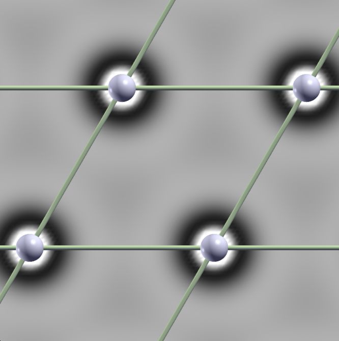
• comparison between pseudopotential (PP) valence-density vs. all-electron densities
(valence and total):
PP valence charge density all-electron valence charge density all-electron total charge density
QE-2021: MaX School on Advanced Materials and Molecular Modelling Example: Day-2/example2.Al/ex2.chdens/3. A magnetic example: Iron bulk Fe has two remarkable features: it is magnetic and it “calls for” an Ultrasoft PP (USPP) since its localized 3d atomic states are very hard. • move to the Day-2/example3.Fe/ directory and read the pw.x input file pw.fe fm.scf.in • the structure is bcc (ibrav=3) with one atom per unit cell • notice (i) variables nspin and of starting magnetization, indicating spin- polarized calculation (nspin=2) with unconstrained total magnetization with only the initial guess for the magnetization given and (ii) variables for metallic system (occupations, smearing, degauss) • notice that this calculation uses GGA (PBE): it is specified inside the PP file (can be guessed from the PP file name), reprinted on output as ”Exchange-correlation” • also notice that with USPP, it is typically needed to set ecutrho > 4⇤ecutwfc (it should be at least 8 to 12 times larger) QE-2021: MaX School on Advanced Materials and Molecular Modelling Example: Day-2/example3.Fe/
3. Magnetic structures

Run pw.x in the usual way (pw.x -in pw.fe fm.scf.in > pw.fe fm.scf.out).
In the output, notice:

• the number of k-points is doubled w.r.t the non-magnetic case: the first set of
  k-points contains spin-up states, the second set spin-down states
    (use verbosity=’high’ in namelist &CONTROL if there are more than 100 k-points)

• in the output notice such lines:

              total magnetization                               =   2.41 Bohr mag/cell
              absolute magnetization                            =   2.60 Bohr mag/cell

    Since there is a single (magnetic) atom per unit cell, the only possible magnetic
    structure is ferromagnetic.

QE-2021: MaX School on Advanced Materials and Molecular Modelling                Example: Day-2/example3.Fe/
3. Magnetic structures: going antiferromagnetic
• To reach antiferromagnetic states, you need to:
– introduce a supercell with two sublattices of di↵erent species of atoms (even if
they are the same, it is important that they are labeled as di↵erent)
– start with opposite initial magnetization for the two sublattices
• Can you write input data for an AFM structure?
hint: split bcc into two simple cubic sublattices, ibrav=1, with two atoms at (0,0,0) and ( 12 , 12 , 12 ).
As a convenience, an antiferromagnetic file is provided (pw.fe afm.scf.in)
You can compare the ferromagnetic and antiferromagnetic files by:
• diff pw.fe fm.scf.in pw.fe afm.scf.in
QE-2021: MaX School on Advanced Materials and Molecular Modelling Example: Day-2/example3.Fe/3.1 Convergence tests for ultrasoft pseudopotential(s)
For computational efficiency, it is convenient to keep ecutwfc as low as possible,
while ecutrho is less critical (look at the CPU time report at the end of an output: there are very
many fftw, depending upon ecutwfc, while a much smaller number of fft depends upon ecutrho)
Set the ecutrho/ecutwfc ratio (dual) to 4, 8, 12 and compute the energy vs
ecutwfc curve. For dual = 4 it will look funny: energy increases with increasing
cuto↵ (see next page), but for a higher dual (i.e. better description of augmentation
charge) the normal behavior is observed.
The corresponding PWTK snippet is:
load_fromPWI pw.fe_fm.scf.in
foreach dual {4 8 12} {
foreach ecut {25 30 35 40 45 50} {
SYSTEM "ecutwfc = $ecut
ecutrho = $ecut*$dual "
runPW pw.fe_fm.scf.$dual.$ecut.in
}
}
QE-2021: MaX School on Advanced Materials and Molecular Modelling Example: Day-2/example3.Fe/ex1.ecut/3.1 Convergence tests for ultrasoft pseudopotential(s)
A PWTK script to make convergence check for USPP is provided, i.e.:
-55.800
• move to directory: -55.805
Day-2/example3.Fe/ex1.ecut/ -55.810
-55.815
Total energy (Ry)
• execute: pwtk ecut.pwtk -55.820
-55.825
• you should obtain such a plot -55.830
(notice that curves for dual = 8 and 12 -55.835
dual=4
dual=8
almost coincide) -55.840
dual=12
25 30 35 40 45 50
ecutwfc (Ry)
Homework: for converged values of both cuto↵s and k-points, you may compare
the stability of iron in the bcc, fcc, hcp phases (the latter being a slightly more
complicated structure)
QE-2021: MaX School on Advanced Materials and Molecular Modelling Example: Day-2/example3.Fe/ex1.ecut/3.2 Density of States (DOS) and Projected DOS (PDOS)
1. move to Day-2/example3.Fe/ex2.dos/ directory and
2. edit the dos.pwtk script and set ecutwfc and ecutrho to appropriate values
3. execute: pwtk dos.pwtk
(this script calculates both total DOS and DOS projected (PDOS) to atomic orbitals)
Total DOS Orbital projected DOS - PDOS
( press in the terminal for the next plot ... )
3
3 majority spin: s-states
majority spin majority spin: d-states
minority spin minority spin: s-states
2 minority spin: d-states
2
1
1
PDOS
0
DOS
0
-1 -1
-2 -2
-3 -3
-8 -6 -4 -2 0 2 4 6 8 -8 -6 -4 -2 0 2 4 6 8
Energy (eV) Energy (eV)
QE-2021: MaX School on Advanced Materials and Molecular Modelling Example: Day-2/example3.Fe/ex2.dos/3.2 Density of States (DOS) and Projected DOS (PDOS)
The scheme to calculate DOS and PDOS consists of:
1. an SCF pw.x calculation (calculation=’scf’)
2. a non-SCF pw.x calculation (calculation=’nscf’), where:
• the same prefix and outdir are used as in the preceding SCF calculation
• a denser k-point mesh is specified
• in this example the linear tetrahedron method is used
(variable occupations=’tetrahedra’)
3. a dos.x calculation to calculate DOS (DOS is written to a file as specified by the fildos
variable in the dos.x input; also here the values of prefix and outdir are the same as for SCF
pw.x calculation)
4. a projwfc.x calculation to calculate PDOS projected to atomic states (this calculation
is analogous to dos.x one, inputs are also very similar; you can compare them as:
• diff dos.Fe.in projwfc.Fe.in
the di↵erence is that dos.x uses the fildos whereas projwfc.x uses the filpdos variable)
Explore the content of fildos and filpdos files!
QE-2021: MaX School on Advanced Materials and Molecular Modelling Example: Day-2/example3.Fe/ex2.dos/You can also read