QUANTIFYING THE QUALITY OF INDOOR MAPS - ISPRS Archives
←
→
Page content transcription
If your browser does not render page correctly, please read the page content below
The International Archives of the Photogrammetry, Remote Sensing and Spatial Information Sciences, Volume XLII-2/W13, 2019
                            ISPRS Geospatial Week 2019, 10–14 June 2019, Enschede, The Netherlands

                                 QUANTIFYING THE QUALITY OF INDOOR MAPS

          Moawiah Assali1, Georgios Pipelidis2∗, Vladimir Podolskiy1, Dorota Iwaszczuk3, Lukas Heinen4, Michael Gerndt1
            1
                 Chair of Computer Architecture and Parallel Systems, Dept. of Informatics, Technical University of Munich,
                          Munich, Germany - muawiya.asali@gmail.com, v.podolskiy@tum.de, gerndt@in.tum.de
             2
                 Software and Systems Engineering Research Group, Dept. of Informatics, Technical University of Munich,
                                               Munich, Germany - pipelidi@in.tum.de
                   3
                       Remote Sensing and Image Analysis Group, Dept. of Civil and Environmental Engineering Science,
                               Technische Universität Darmstadt, Germany - iwaszczuk@geod.tu-darmstadt.de
                                        4
                                            BMW Group IT, Munich, Germany - lukas.heinen@bmw.de

                                                           Commission I, WG I/7

KEY WORDS: Quality Metrics, Indoor Map, Robot Map, Dynamic Quality Assessment

ABSTRACT:

Indoor maps are required for multiple applications, such as, navigation, building maintenance and robotics. One of common methods
for map generation is laser scanning. In such maps, not only geometry of the map is of interest, but also its quality. This study aims
at developing methods for real-time generation of indoor maps using features extracted from pointclouds obtained by a robot with
their simultaneous quality assessment. We investigate, how this quality can be quantified for feature-based maps. First, we introduce
a method for modeling 2D maps into 3D models that enable their usage for localization. Second, we review and evaluate a number of
algorithms that can enable us to address features in a map. Hence, we enable the generation of objects from a pointcloud that has been
sensed. Finally, we study several aspects of the map quality and we formalize them into metrics that can be applied to quantify their
quality.

                         1. INTRODUCTION                                 difficult for storage and useless in some analysis where more ab-
                                                                         stract or vector data as well as semantics are required. Therefore
Indoor maps are used in various applications, such as, naviga-           feature based representation and their quality are more suitable
tion, building maintenance and robotics. One of the popular tech-        representation. In order to consider the quality of the map dur-
niques to obtain indoor maps is laser scanning. In order to seam-        ing the mapping process, both, mapping and quality assessment
lessly sense larger indoor spaces including multiple rooms and           should be performed in real time. Frank and Ester (2006) propose
corridors, mobile platforms are used. In such case, the indoor           a method to quantify the quality of a map after generalization
environment can be mapped using an approach called Simultane-            takes place. They analyze many deformations that may result af-
ous Localization And Mapping (SLAM) introduced by Durrant-               ter generalization and propose an approach to specify map quality
Whyte et al. (1996). Pointclouds obtained in that way can be             based on inaccuracies that can be detected. They provide a list of
compared with already existing maps, which can be used for po-           possible map operations that may result in increasing the uncer-
sitioning or map update. For this purposes, not only the geometry        tainty. According to them, those operations are: (1) Elimination,
of the existing an new map is needed, but also the quality of this       when all objects are not displayed, (2) Exaggeration, when ob-
map is of high interest, as it is one of the attributes which should     jects are enlarged, (3) Aggregation/Division, when multiple ob-
be considered during the map usage as well as it should be consid-       jects are combined or larger objects are decomposed to smaller
ered during the matching and co-registration. Sester and Förstner       ones, (4) Displacement, when objects have been shifted, (5) Re-
(1989); Iwaszczuk and Stilla (2017).                                     duction when object have been eliminated, (6) Typification, when
                                                                         objects are described via typical patterns.
Even though a lot of research focuses on map construction meth-
ods Karagiorgou and Pfoser (2012), there is a lack of methods            According to Pipino et al. (2002), quality metrics can be catego-
that can enable the quantification of the quality of a robot gener-      rized into groups based on objective or subjective approaches.
ated map. Additionally, publications that focus on map evaluation        They call the metrics subjective, when they focus on the user
(Frank and Ester, 2006; Podolskaya et al., 2009) do not provide          needs and objective when they are task-dependent or indepen-
a detailed analysis and comparison of criteria to be used for map        dent. They apply this analysis on maps by assigning weights to
quality assessment. Tran et al. (2019) focus on geometric com-           each metric based on its importance for a specific user segment.
parison of a 3D indoor model with a reference. However, we need          Schwertfeger (2012) compares robot maps to ground truth maps.
to consider the fact that maps may be used for a number of dif-          He makes use of map quality attributes such as:(a) Global Ac-
ferent applications and require different methods of comparison.         curacy that is defined by the difference in distance between the
                                                                         actual map feature and its corresponding estimated distance, (b)
In order to determine the quality of a map, the quality of the 3D
                                                                         Relative Accuracy that describes the amount of transformation
pointcloud can be calculated (Karam et al., 2018). 3D pointcloud,
                                                                         (i.e. shifting, rotating, etc) that has been introduced to the gener-
however, is an unorganized form of the 3D map and therefore
                                                                         ated map, (c) Local Consistencies that studies relative positions
  ∗ Corresponding      author                                            changes between objects, (d) Coverage, that describes the per-

                                                     This contribution has been peer-reviewed.
                        https://doi.org/10.5194/isprs-archives-XLII-2-W13-739-2019 | © Authors 2019. CC BY 4.0 License.                   739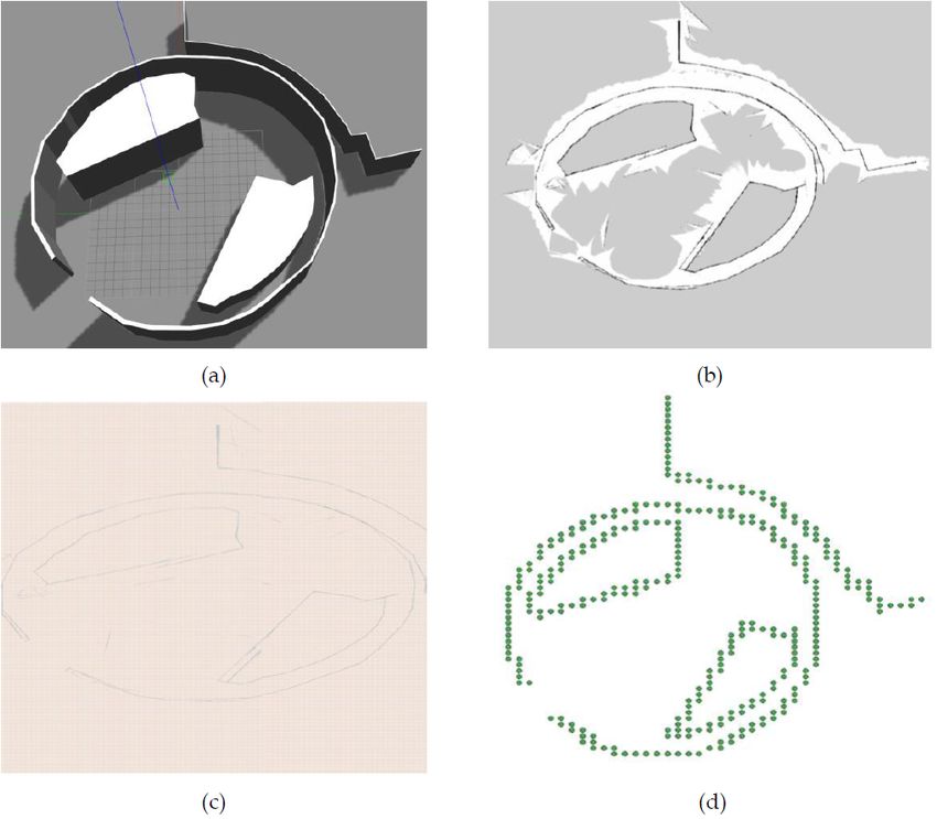
The International Archives of the Photogrammetry, Remote Sensing and Spatial Information Sciences, Volume XLII-2/W13, 2019
ISPRS Geospatial Week 2019, 10–14 June 2019, Enschede, The Netherlands
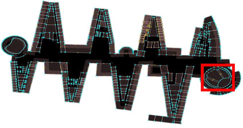
centage of features that have been mapped, (e) Resolution Quality 3. Scanning the environment via LiDAR sensors (Figure 1c).
that describes the number of map features that could be identified
based on the originals. 4. reasoning on the LiDAR sensed values and extraction of the
point cloud (Figure 1d).
Birk (2009) focuses on grid maps quality analysis. He introduces
a metric that he calls ‘brokeness’, responsible to control the num- Using this approach, we can ensure that the generated 3D map
ber of regions in a map as well as their spatial relations. He argues and 3D LiDAR poincloud are in the same coordinate system.
that a common error in map generation is rotated regions or par-
ticular regions that have been rotated due to technical problems
such as slipping wheels in a robot. When applying cross entropy
between cells at such situations will result in very low quality val-
ues despite the fact local contents of the wrong rotated room are
correct. Brokeness is introduced to quantify such errors, based on
a ground truth map. Zhang et al. (2011) propose a metric called
Feature Similarity Index for Image Quality Assessment - FSIM
for assessment of low level detail of an image, similar to what
the human visual system perceives. Their approach consist of
phase congruency, which specifies the local significance of a fea-
ture and image gradient magnitude. that involves three gradient
operators, such as Sobel, Prewitt, and Sharr operators as for the
estimation of the gradient magnitude. Cakmakov and Celakoska
(2004) discuss shape similarity of detected objects in an image or
a map. They distinguish two curve types, closed and free, where
Closed are those that describe an objects, while free which are
not closed, i.e. have no closing point. In such cases, a part of the
curve should be imagined as to be able to compare with others.
The authors define four perspectives possibilities for the match-
ing process: (a) Transformational - where representations such Figure 1. Pointcloud building: a) blender model of the
as turning functions are used, (b) Geometrical - where polygon environment; b) model in the Gazebo simulation tool; c)
representations are used. (c) Structural - where graph matching scanning the indoor environment via robot’s LiDAR sensors that
techniques are used. (d) Quantitative - where closed curves are Turtlebot3 robot is equipped with. The fourth step, in 1.(d), is to
identified for shape description. reason on the LiDAR sensed values and extract a point cloud
1.1 Contribution After the pointcloud is acquired, points are first clustered into
lines, which are later clustered into polylines or polygons. Clus-
In this study we aim at developing a set of methods for real-time tering points into objects is achieved via buffering, where each
generation of indoor maps using features extracted from point- point’s boundaries are extended until they overlap with bound-
clouds acquired by a robot with their simultaneous quality assess- aries of another point or reach a maximum threshold. After points
ment. Then we investigate, how this quality can be quantified for are structured into groups according to their nearest neighbors, a
feature-based maps. First, we introduce a method for modeling second level of clustering is applied that enables us to separate
2D maps into 3D models that enable their usage for localization. points that belong to different polygons .
Second, we review and evaluate a number of algorithms that can
enable us to address features in a map. Hence, we enable the gen- Based on the clustering results, polygons are recognized. We de-
eration of objects from a pointcloud that has been sensed. Finally, vised three different strategies for polygon specification. Those
we study several aspects of the map quality, and review existing approaches are based on a number of existing algorithms, such
methods for quality quantification. Based on analysis of exist- as the Concave Hull, Convex Hull, and Dijkstra Algorithm. We
ing metrics, we identify a need to introduce a new quality metric used and tested all the three algorithms and a detailed evaluation
- Characteristic Similarity, in order to quantify the rotation mis- is available in the evaluation section. Examples of the concave
match, which is not covered by existing metrics. hull and convex hull algorithms are presesnted in Figure 2.
2.1 Concave Hull
2. 3D MAP GENERATION
This algorithm aims to describe the region, which is occupied
We propose an approach to generate a dataset for our investiga- by a set of points. The algorithm operates based on a smooth-
tion based on Open Street Maps. We use them, to generate both: ness parameter that controls the corners of a polygon and their
the reference the 3D map and the LiDAR pointcloud. The re- allowed irregularity. For example, a polygon may be assembled
quiered data is being generated in four steps, as depicted in Figure from points that their interior angles are less than or equal to 180
1. degrees. Hence, a concave polygon is the polygon that surrounds
a set of points by the smallest possible area. An example of the
concave hull algorithm is available in Figure 2a.
1. Blender model of the environment (OSM2World, n.d.) (Fig-
ure 1a). 2.2 Convex Hull
2. Model introduced to the Gazebo simulation tool (Gazebo, The concave hull based algorithm operates based on the same
n.d.) (Figure 1b). principles with concave hull. Its main difference from Concave
This contribution has been peer-reviewed.
https://doi.org/10.5194/isprs-archives-XLII-2-W13-739-2019 | © Authors 2019. CC BY 4.0 License. 740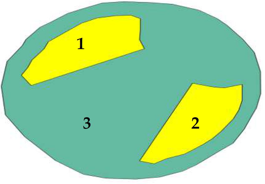
The International Archives of the Photogrammetry, Remote Sensing and Spatial Information Sciences, Volume XLII-2/W13, 2019
                               ISPRS Geospatial Week 2019, 10–14 June 2019, Enschede, The Netherlands

Hull is that instead of the level of smoothness, it tunes the tight-   The offset between those distances reflects the location similar-
ness of a polygon. As result, a polygon obtained through the           ity for each object, from which, it eventually computes a global
concave approach tends to obtain tighter areas around the same         Location Similarity value for the entire map as
set of points, when compared to a convex approach. An example
                                                                                                       [ pm=1 LSi (A, B)]
                                                                                                        P
of the convex hull algorithm is available in Figure 2b.                             LS(A, B) = 1 −                        ,          (2)
                                                                                                                n
                                                                       where LSi (A, B) is location similarity value for the ith object of
                                                                       maps A and B and n describes the number of objects in the map.

                                                                       3.2   Semantic Content Similarity - SCS

                                                                       This metric, introduced by Frank and Ester (2006), aims to quan-
                                                                       tify neglected objects that have been either merged with others,
                                                                       have not being included or their only partial represented in the
                                                                       map. This metric operates by estimating the Voronoi entropy of
Figure 2. Example of polygons obtained via the concave hull (a)        the identified objects as
           and convex hull (b). Franois Blair (n.d.).
                                                                                                 X
                                                                                     V Ei (A) =      ([Pi ∗ ln(Pi ) ∗ %V ]),        (3)
2.3    Clustering Based on the Dijkstra Algorithm
                                                                       where V Ei (A) indicates the entropy of the ith object category in
Dijkstra is commonly used to calculate the shortest path between
                                                                       the map A, %V is the percentage of Voronoi area of one object
two points or locations. However, in our scenario, it is used to
                                                                       class with respect to the entire Voronoi area, and P is the number
determine the sequence among the set of points, necessary for
                                                                       of objects of the category i. More specifically, this metric oper-
forming a polygon. More specifically, this step is executed fol-
                                                                       ates by first categorizing objects according to the their occupied
lowing three different sub-steps. The first step is to generate the
                                                                       area, usage and shape and then it estimates the entropy for each
sequence of points, by marking each feature with a value that rep-
                                                                       of the categories on the reference, as well as the generated map.
resents its location in reference to the previous nearest point. The
                                                                       Finally, it estimates the rate of change of Entropy between those
second step is to generate lines between all points, based on the
                                                                       two maps.
sequencing occurred above. The last step, is to fill enclosed areas
via the connected lines, which eventually enables us to reveal the     The final SCS score, is computed as
polygons.
                                                                                                    min[V Ei (A), V Ei (B)]
                                                                                   SCS(A, B) =                                          (4)
                                                                                                    max[V Ei (A), V Ei (B)]
                 3. QUALITY ASSESSMENT
                                                                       where V Ei (A) and V Ei (B) describes the Voronoi entropy of
In this section, we describe the set of quality metrics that we ap-    the maps A and B respectively. This formula allows to obtain the
plied to the dynamically generated maps to quantify their quality.     ratio of entropy change. When reference and new maps obtain
                                                                       the same entropy values, then the two maps are identical.
3.1    Location Similarity - LS
                                                                       3.3   Characteristic Similarity - CS
This metric, introduced by Frank and Ester (2006), aims at quan-
tifying the difference between locations of the same feature in the    This metric is introduced by us and aims at quantifying how each
generated map, when compared against the reference map (dis-           polygons attributes preserved after generalization.
placement error). The metric makes use of Voronoi cells, aiming
to reveal offsets between objects, by estimating the shifting that     The most important step here is to design a suitable list of char-
has occurred to the center of gravity between each object. The         acteristics to be used for comparison:
main idea behind Voronoi cells is to divide the map area into seg-
ments of equal surface, while the center of each cell remains to
be the object’s center.                                                  • Prepare and compute an attribute list which supports the area
                                                                           and perimeter of a polygon.
The component’s execution begins by applying the Voronoi algo-
rithm on the map and obtain a list of neighbors for each feature.        • Compare each polygon with its corresponding one in the ref-
The next step is to calculate distances between each feature and           erence map .
its direct neighbors. Finally, it computes the differences of those
                                                                         • Provide each attribute with a specific weight reflecting its
distances as
                                                                           importance.
                         [ pm=1 | distAmax(dist(i))
                                        (i,m)−distB (i,m)
                          P
                                                          |]
     LSi (A, B) = 1 −                                        ,  (1)
                                         p                             After obtaining a numerical list of attributes for each object in the
                                                                       map, the metric
where, LSi (A, B) is a value that describes the location similar-
ity of the ith object of map A and map B. The distance between                                       min[Ci (A), Ci (B)]
two objects i and m of the map A and map B is described by                           CS(A, B) =                          ,              (5)
                                                                                                     max[Ci(A), Ci(B)]
distA (i, m) and distB (i, m) respectively. The maximum dis-
tance between two objects is expressed by max(dist(i)) and fi-         where Ci is characteristic of ith element in maps A and B. The
nally, the number of neighbors of an object is described by p.         value is normalized to be between 0 and 1.

                                                 This contribution has been peer-reviewed.
                    https://doi.org/10.5194/isprs-archives-XLII-2-W13-739-2019 | © Authors 2019. CC BY 4.0 License.                     741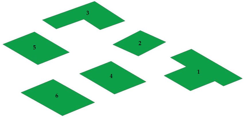
The International Archives of the Photogrammetry, Remote Sensing and Spatial Information Sciences, Volume XLII-2/W13, 2019
                               ISPRS Geospatial Week 2019, 10–14 June 2019, Enschede, The Netherlands

3.4    Shape Similarity - SS

This metric was introduced by Frank and Ester (2006). Its goal
is to quantify the difference of the shape of the objects that be-
long to the maps. For achieving this, it makes use of the turning
function. The turning function is a step-function that describes
a shape by plotting its perimeter against its slope, steps on the
function reflect rotations that a perimeter performs to construct
the shape.

More specifically, this subcomponent is implemented by first es-
timating the turning function of each object using the Formula
6. Later, it subtracts the turning function of each object from                                Figure 3. Test area
each of object’s turning function on the reference map, since the
area between the two curves describes the difference between two        In Figure 4 it can be seen the extracted polygons. They were
turning functions. Finally, it normalizes this value based on the       extracted via the concave hull algorithm, with tightness range be-
maximum difference.                                                     tween 0.36 and 0.51. Table 1 lists the obtained quality results for
                                                                        all polygons.

                                Area(Ni )
  SSi (Ni ) = 1 −                                                (6)
                     max([Area(T Fi , A), Area(T Fi , A)])

where T Fi , A is the turning function that describes the shape of
the ith object in the map A, while Ni is the area between the two
turning functions.

3.5    Polygon Assessment - PA
                                                                          Figure 4. Polygons extracted in test area via the concave hull
Polygon Assessment, introduced by Podolskaya et al. (2009), is
                                                                                                   approach
an aggregation of the Shape Similarity and Characteristic Simi-
larity, with an additional metric, the Vertices of each object. It            Quality Metric   Polygon 1     Polygon 2     Polygon 3
expresses the trade-off between the reduced amount of data and                LS               0.98          0.96          0.99
the generalized characteristics of the map.                                   CS               0.95          0.95          0.89
                                                                              SS               0.77          0.90          0.89
This metric is calculated by first computing the turning function             PA               0.79          0.86          0.77
for each object in order to compute the shape similarity, as well
as computing the area for each available object for assessing the             Table 1. Calculated quality measures for each polygon
characteristic similarity. Finally, we compute the number of ver-             calculated using Concave Hull approach (Scenario 1)
tices for each available object. The final numerical metric value
can be then computed by                                                 As can be seen in Table 2 the obtained quality scores are high,
                                                                        since the robot did not suffer from displacement shifts or errors.
                                                                        We can notice, that the Shape Similarity (SS) and Polygon As-
           P A = WSS ∗ SS + WCS ∗ CS + WV ∗ V,                   (7)    sessment (PA) values are low compared to other metrics. SS is
                                                                        highly dependable on vertices because it is computed based on a
where SS is the shape similarity, CS is the characteristic similar-     turning function. We could observe that large polygons contain-
ity and V describes the vertex characteristics, while WSS , WCS         ing large number of vertices achieve the lowest SS values. Also
and WV are weights for each corresponding metric.                       PA metric uses vertices as an integral part of its computation in
                                                                        conjunction with the Shape Similarity.

                       4. EVALUATION                                    4.1   Scenario 2

Two different shaped areas were selected to evaluate the devel-         The second scenario builds on the outdoor area from the Rus-
oped framework. The data was acquired by the Turtlebot3 us-             sel Road in London (Figure 5). This scenario was chosen due to
ing the Gazebo simulation tool Gazebo (n.d.). The two scenarios         the presence of inner and outer angles that follow L or T shape.
were composed based on the variety of polygons in these areas:          Such shapes allow to evaluate the limits of the proposed algo-
                                                                        rithm when it is applied to the areas encompassing concave and
Scenario 1 The first scenario is placed at Technical University         convex hulls. Additionally, in this scenario objects have more di-
of Munich, which is marked red square in Figure 3. The room             rect neighbors. This is expected to influence the quality of the
is a lecture hall and it consists of three polygons, which are com-     result due to the additional displacement of the objects. How-
posed by a collection of arc, circular and straight vertices, the two   ever, more neighbors imply more relations which increases the
smaller polygons are overlapping with the larger polygon, which         map processing time.
influences the Voronoi diagrams generation. Additionally, the
place consists of narrow corridors and cantilever points, which         In Figure 6 can be seen the identified polygons, while in Table
could cause a drop to the LiDAR accuracy.                               3 the results for the second scenario using polygon specification

                                                 This contribution has been peer-reviewed.
                    https://doi.org/10.5194/isprs-archives-XLII-2-W13-739-2019 | © Authors 2019. CC BY 4.0 License.                    742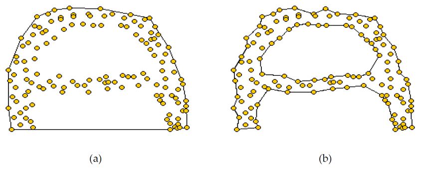
The International Archives of the Photogrammetry, Remote Sensing and Spatial Information Sciences, Volume XLII-2/W13, 2019
                            ISPRS Geospatial Week 2019, 10–14 June 2019, Enschede, The Netherlands

                      Concave     Convex      Dijkstra                                        Concave      Convex     Dijkstra

              LS        0.98        0.98        0.97                                   LS        0.99       0.99        0.99
             SCS        0.99        0.98        0.98                                 SCS         0.99       0.97        0.99
              CS        0.93        0.92        0.84                                   CS        0.97       0.94        0.87
              SS        0.78        0.60        0.29                                   SS        0.37       0.59        0.03
              PA        0.80        0.78        0.56                                   PA        0.62       0.70        0.45

  Table 2. Map quality calculated based on introduced quality                           Table 3. Scenario 2 - Final Results
                    measures (Scenario 1)
                                                                         Qual. Metr.     Pol 1     Pol 2   Pol 3    Pol 4      Pol 5   Pol 6
                                                                         LS              0.99      0.99    0.99     0.99       0.99    0.98
                                                                         CS              0.98      0.97    0.98     0.99       0.98    0.93
                                                                         SS              0.13      0.53    0.24     0.80       0.21    0.261
                                                                         PA              0.54      0.7     0.60     0.76       0.59    0.58

                                                                              Table 4. Calculated quality measures for each polygon
                                                                              calculated using Concave Hull approach (Scenario 2)

                                                                        ues for the algorithm) may result in a situation where line seg-
                                                                        ments start breaking around local cantilever points creating more
                                                                        additional vertices deforming the shape which in turn deforms the
                                                                        quality of the shape. This observation implies that a smoothness
                                                                        value should be chosen to avoid two extremes of having many
                                                                        broken segments producing new unnecessary vertices and cutting
                                                                        inner angles in a way that deforms shapes.

   Figure 5. Scenario 2 - Customized Russel Road Buildings              5.1   Straight Trajectories:

with Concave Hull, Convex Hull, and Dijkstra Algorithm are pre-         This property is similar to the previous one in its effect upon qual-
sented. The quality evaluation provides a better picture of how         ity metrics. The main observation is that when a relatively long
the polygons affect the quality of the extracted map, using vari-       straight trajectory is considered, a robot may add additional ver-
ous metrics Table 4.                                                    tices that are not displayed on a corresponding reference map.
                                                                        Another observation is that when a robot passes the same loca-
                                                                        tion more than once, new vertices may be introduced, each with
                                                                        a small added shift in the corresponding turning function. Shape
                                                                        Similarity and Polygon Assessment metrics are mostly affected
                                                                        by this type of trajectory.

                                                                        Overlapping Polygons: These polygons increase the difficulty
                                                                        to capture boundaries between objects. They also may change
  Figure 6. Polygons extracted in test area via the concave hull
                                                                        how a relative location for one object is computed as a Loca-
                           approach.
                                                                        tion Similarity metric may take other forms to represent an object
                                                                        (other than a center of gravity). Location Similarity is the most
                        5. DISCUSSION                                   affected by this feature of the map (Table 1, low LS value for
                                                                        polygon 3).
The collected results enabled us to notice that the following prop-
erties of both explained scenarios affect specific quality metrics:     5.2   Narrow Corridors

Arc Trajectories: One may notice that the robot did not manage to       Presence of a narrow passage on a map may force two indepen-
capture exact vertices for this type of trajectory. In turn, this di-   dent polygons to merge. This will result in a decreased object
rectly affected the shape similarity and the polygon assessment         count and relative importance after scan. Such a map feature af-
quality metrics. The first metric is affected as a result of cu-        fects Semantic Content Similarity metric as it takes into account
mulative angles being represented in the corresponding turning          how objects are categorized before and after a scan. Considered
function. The second one is affected because the shape similar-         examples of narrow passages in both scenarios did not, however,
ity is one of its components and it already considers the number        generate cases with merged or eliminated objects.
of Vertices in its computations. Concave and Convex Hull poly-
gons were less affected by this property than Dijkstra because of       5.3   Complex Rounding
Dijkstra’s ability to capture sharp segments that contribute to a
higher deformation of the shape. The tightness parameter reflects       This map feature is similar to Narrow Corridors in its effect on
how far the difference is between Concave and Convex Hulls ap-          the ability to separate objects. Dense area of points causes such
proaches. Increasing the tightness factor (lower smoothness val-        an issue. Presence of a complex rounding increases the burden

                                                This contribution has been peer-reviewed.
                   https://doi.org/10.5194/isprs-archives-XLII-2-W13-739-2019 | © Authors 2019. CC BY 4.0 License.                       743
The International Archives of the Photogrammetry, Remote Sensing and Spatial Information Sciences, Volume XLII-2/W13, 2019
ISPRS Geospatial Week 2019, 10–14 June 2019, Enschede, The Netherlands
to produce good shapes as the perimeter may be affected by de- even more importance, as proposed qualities can be used to as-
formed vertices. Shape Similarity and Semantic Content Simi- sess, whether the match with a reference map can be correct or
larity are affected in these cases. The first scenario shows some not. To implement such approach, a single quality value would
cases where the presence of a complex rounding around inner be easier to handle. Therefore, our future efforts will turn towards
polygons affected the shape a little bit thus introducing a drop in combining the individual results of each metric results in a final
quality metrics. quality value assisting in marking a map as accepted or not. Fur-
thermore, we plan to work on a quality measure for assessment
5.4 Cantilever Points of the outdoor-indoor co-registration.
The presence of these points creates challenges to produce exact
perimeter and shapes. It affects Shape Similarity and Character- References
istic Similarity metrics. These points can be produced as a result
Birk, A., 2009. A quantitative assessment of structural errors in
of an algorithm used to generate polygons. Each algorithm may
grid maps. Autonomous Robots 28(2), pp. 187.
differ in how it deals with these points but one may notice that
Concave Hull is the least affected by this property. Cakmakov, D. and Celakoska, E., 2004. Estimation of curve simi-
larity using turning functions. International Journal of Applied
5.5 Inner Angles Mathematics 15, pp. 403–416.
Inner angles deform the whole polygon shape if wrong tightness Durrant-Whyte, H., Rye, D. and Nebot, E., 1996. Localization
values are used. As we notice in the second scenario, polygons 1 of autonomous guided vehicles. In: G. Giralt and G. Hirzinger
(eds), Robotics Research, Springer London, London, pp. 613–
and 3 have inner angles and they generated low quality values in 625.
Concave Polygons case because of high value of tightness. Tight-
ness in these cases managed to capture better inner angles but it Frank, R. and Ester, M., 2006. A quantitative similarity mea-
results in breaking straight line segments around local cantilever sure for maps. In: Progress in spatial data handling, Springer,
points. pp. 435–450.
Franois Blair, n.d. Everything you always
5.6 Relative Neighbors
wanted to know about alpha shapes but were
afraid to ask. http://cgm.cs.mcgill.ca/ god-
This property shows how the choice of metrics may affect time fried/teaching/projects97/belair/alpha.html. accessed online
needed to generate quality values. At some cases, not all of map 04/2019.
objects are important to be included into calculations. For in-
stance, checking quality for specific parts of the map or neglect Gazebo, n.d. https://gazebosim.org/. accessed online 04/2019.
tiny objects at specific use cases. Moreover, in use cases where Iwaszczuk, D. and Stilla, U., 2017. Camera pose refinement by
location is already known and the shape matters, Location Simi- matching uncertain 3d building models with thermal infrared
larity can be dropped out. image sequences for high quality texture extraction. ISPRS
Journal of Photogrammetry and Remote Sensing 132, pp. 33–
47.
6. CONCLUSION
Karagiorgou, S. and Pfoser, D., 2012. On vehicle tracking data-
This paper proposed an approach to quantify the quality of robot based road network generation. In: Proceedings of the 20th
maps that we obtain from different environments. First, we mod- International Conference on Advances in Geographic Infor-
eled the environment and acquired its corresponding pointcloud mation Systems, ACM, pp. 89–98.
by performing a robot scan. To obtain a 3D indoor map, three Karam, S., Peter, M., Hosseinyalamdary, S. and Vosselman, G.,
different algorithms enabling the modeling of detected objects 2018. An evaluation pipeline for indoor laser scanning point
(Concave Hull, Convex Hull and Dijkstra Algorithm) were ex- clouds. ISPRS Annals of Photogrammetry, Remote Sensing
plored. As the core contribution of this paper, we provided a se- and Spatial Information Sciences IV-1, pp. 85–92.
ries of quality metrics that aim to capture different aspect of the
generated polygons. Finally, we analyzed which aspects of map OSM2World, n.d. http://osm2world.org/. accessed online
04/2019.
quality can be visible in which metric. Our approach was tested
against different environments. Pipino, L. L., Lee, Y. W. and Wang, R. Y., 2002. Data quality
assessment. Communications of the ACM 45(4), pp. 211–218.
We showed, that proposed quality quantification approaches are
suitable to assess a feature based map obtained by a robot. Be- Podolskaya, E. S., Anders, K.-H., Haunert, J.-H. and Sester, M.,
sides, by defining quality metrics, we are enabled to identify 2009. 16 quality assessment for polygon generalization. Qual-
ity Aspects in Spatial Data Mining p. 211.
deformations that may happen through generalization processes,
also in the reference map. Schwertfeger, S., 2012. Robotic mapping in the real world: Per-
formance evaluation and system integration. PhD thesis, Ja-
cobs University Bremen.
7. FUTURE WORK
Sester, M. and Förstner, W., 1989. Object location based on
A big topic for 3D indoor maps is georeferencig and relation to uncertain models. In: H. Burkhardt, K. Hähne and B. Neu-
outdoor maps. This is particularly important for navigation pur- mann (eds), Muster Erkennung 1989, 11th DAGM-Symposium,
poses, where seamless transitions between outdoor and indoor Springer-Verlag London, pp. 457–464. ISBN:3-540-51748-0.
environment are necessary. In indoor, a high-quality and up-to- Tran, H., Khoshelham, K. and Kealy, A., 2019. Geometric com-
date map is even more important than in outdoor, as indoor nav- parison and quality evaluation of 3d models of indoor environ-
igation cannot rely on GNSS technology and often must be sup- ments. ISPRS Journal of Photogrammetry and Remote Sensing
ported my map matching. In this context, the map quality wins 149, pp. 29 – 39.
This contribution has been peer-reviewed.
https://doi.org/10.5194/isprs-archives-XLII-2-W13-739-2019 | © Authors 2019. CC BY 4.0 License. 744The International Archives of the Photogrammetry, Remote Sensing and Spatial Information Sciences, Volume XLII-2/W13, 2019
ISPRS Geospatial Week 2019, 10–14 June 2019, Enschede, The Netherlands
Zhang, L., Zhang, L., Mou, X. and Zhang, D., 2011. Fsim: A
feature similarity index for image quality assessment. IEEE
Transactions on Image Processing 20(8), pp. 2378–2386.
This contribution has been peer-reviewed.
https://doi.org/10.5194/isprs-archives-XLII-2-W13-739-2019 | © Authors 2019. CC BY 4.0 License. 745You can also read