Weakly-supervised multi-class object localization using only object counts as labels
←
→
Page content transcription
If your browser does not render page correctly, please read the page content below
Weakly-supervised multi-class object localization
                                                    using only object counts as labels

                                                              Kyle Mills                                        Isaac Tamblyn
                                                          Faculty of Science                         National Research Council Canada
                                             University of Ontario Institute of Technology                 Ottawa, Ontario, Canada
arXiv:2102.11743v1 [cs.CV] 23 Feb 2021

                                                       Oshawa, Ontario, Canada                    Vector Institute for Artificial Intelligence,
                                              Vector Institute for Artificial Intelligence,               Toronto, Ontario, Canada
                                                       Toronto, Ontario, Canada                           isaac.tamblyn@nrc.ca
                                                       kyle.mills@uoit.net

                                                                                       Abstract
                                                  We demonstrate the use of an extensive deep neural network to localize instances
                                                  of objects in images. The EDNN is naturally able to accurately perform multi-class
                                                  counting using only ground truth count values as labels. Without providing any
                                                  conceptual information, object annotations, or pixel segmentation information, the
                                                  neural network is able to formulate its own conceptual representation of the items
                                                  in the image. Using images labelled with only the counts of the objects present,
                                                  the structure of the extensive deep neural network can be exploited to perform
                                                  localization of the objects within the visual field. We demonstrate that a trained
                                                  EDNN can be used to count objects in images much larger than those on which
                                                  it was trained. In order to demonstrate our technique, we introduce seven new
                                                  datasets: five progressively harder MNIST digit-counting data sets, and two data
                                                  sets of 3d-rendered rubber ducks in various situations. On most of these datasets,
                                                  the EDNN achieves greater than 99% test set accuracy in counting objects.

                                         1   Introduction
                                         The goal of automated object localization research is to take a two-dimensional projection of a scene
                                         (e.g. a photograph) and construct a spatial density map, indicating where in the image the objects
                                         of interest appear. The integral of this density map can be evaluated to arrive at a count of the
                                         number of objects of various types present in the full three-dimensional area [1]. There are numerous
                                         applications where accurate counting of objects from a visual camera signal is beneficial, such as
                                         population monitoring in the Seregeti[2], counting humans in crowded locations [3, 4, 5, 6, 7, 8], or
                                         counting bacteria on microscope slides [9]. In order to train supervised computer vision and machine
                                         learning methods for this task, labels are required. In the most strongly-supervised techniques, each
                                         pixel is assigned to a class and the task is called segmentation, with the neural network tasked at
                                         predicting labels at pixel resolution. Coming in slightly weaker are datasets labelled with bounding
                                         boxes around objects and the problem is cast as one of detection. More weakly-supervised techniques
                                         that use point annotations have been employed to count cells [10, 11, 12, 13, 14, 9, 15, 16], cars
                                         [17, 18, 19], and penguins [20, 16], among other things. Point annotations are more appropriate when
                                         object occlusion is present and bounding boxes or pixel-specific labels would overlap significantly
                                         [13]. The main difficulty with these approaches lies in obtaining the detailed annotation labels (e.g.
                                         bounding boxes or positions). These annotations are traditionally provided by humans, such as the
                                         task of clicking on penguins in the arctic [20]. Crowdsourcing this tedious work has become common,
                                         but with non-experts and anonymous users providing the labels, a training set could easily become
                                         fouled with erroneous labels, making training an accurate model difficult [21]. It is substantially
                                         easier to arrive at a count of the number of objects present in the field of view than it is to assign all
                                         pixels to class or draw bounding boxes around objects.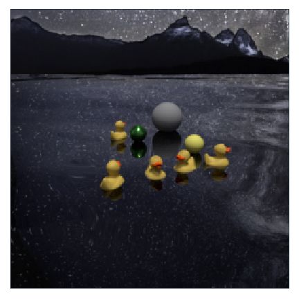
1.1   Related work

Patch-based counting and localization approaches are common, with the standard approach being to
cast the problem as a density-map regression problem. For example, Refs. [10, 19, 18, 9] blur point
annotations to construct a density map. Then they train a regression model to, acting on a single patch
at a time, reproduce this density map. Once the model is trained, a density map can be constructed
from new images, providing localization information, and the integral of the density map can provide
total count information.
Our application aims to make the task even simpler; knowing only the number of objects present in
an image and using this as a label, we train an end-to-end deep learning model capable of achieving
both accurate multi-class counting and multi-class localization of objects. One of the benefits of
using only the raw object counts is that count information is more easily obtained than precise
location annotations, and furthermore, the count signal need not originate from the visual signal itself.
Measurements from other devices, e.g. weight sensors, optical tripwires, etc. can be used as labels
to train a model operating on the visual signal. Unlike other similar approaches [22], this approach
relies only on a single scalar label, and ground truth segmentation data is not required for obtaining
object localization or counting. Once trained, the model can be applied to arbitrarily large images.
Because the neural network only acts on a small subset of the input image, the actual convolutional
neural network model can be relatively small, and the systematic way in dividing input images into
evenly-sized patches is very easy to implement.

2     Methods

Extensive deep neural networks (EDNN) were proposed by Mills, et. al [23] as a way to capture the
extensive nature of physical properties in physics and chemistry applications. An extensive property
is one that scales linearly with system size (such as number of objects, or total energy in the case of
chemistry applications), with the obverse being an intensive quantity (such as temperature or density).
The EDNN technique itself is relatively simple: break the input image x ∈ RW ×H×d (where d is
the number of channels, e.g. 1 for grayscale and 3 for RGB) into non-overlapping patches of size
f × f × d, called focus regions. These focus regions are then padded with a border of width c, adding
“context” around the non-overlapping patches. Each (f + 2c) × (f + 2c) × d “tile” is then fed through
the same neural network, outputting a single number for each tile. These results are summed and
the final summed value is used as the “prediction” against which to compute the loss and perform
back-propagation. The effect of this technique is that the neural network only needs to learn to predict
a fractional contribution of the final object count. The neural network learns automatically how to
treat the overlapping context regions so as not to double count contributions. Furthermore, since each
tile is comprised of non-overlapping focus regions, one can consider the neural network output for a
single tile the fractional count of the number of objects present and a density map can be constructed
over the original image at a resolution determined by the focus size f . In the case of small focus, this
can enable the precise localization of objects in the image.
We have designed multiple data sets through which we demonstrate the EDNN-counting and localiza-
tion. The MNIST variants are constructed by extracting 4800 examples of each of the ten numerals
from the original MNIST dataset. For each of the ten digits, 480 members are reserved for the testing
sets and 4320 are used to construct the training sets (i.e. no unique MNIST example is present in
both the training and testing sets) The examples are constructed by choosing a random number Ni
between 0 and Lmax for each numeral i present in the data set. This will serve as the label. Ni digits
are then chosen randomly from either the testing or training subset and are composited randomly on
an empty 256 × 256 pixel image through element-wise summation. In the case where occlusion is
permitted, pixel values are clipped at 255. The images are saved as greyscale 8-bit PNG images, with
labels in a separate JSON file.
The RD-2 dataset is generated using a script inspired by the CLEVR [25] dataset, using Blender to
perform the 3d rendering. For each of the label-scene pairs (e.g. “5 ducks, 2 balls, mountain scene”),
we generated 1024 images by randomly placing, scaling, and rotating the appropriate number of
ducks and balls. 896 images of each scene-label pair are used for training and 128 for testing. The
RD-1 dataset is a subset of the RD-2 dataset (the examples with zero balls). The images are generated
at a resolution of 256 × 256 pixels and stored in RGB (3 channel) 8-bit PNG images. Labels are
stored in a separate JSON file.

                                                   2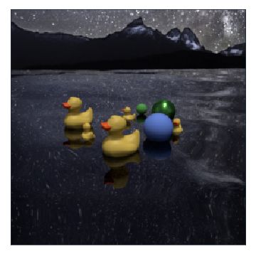
(a)                    (b)                      (c)                       (d)

                  (e)                          (f)                            (g)
Figure 1: An example image from each of the 7 datasets presented in this paper. The datasets are
described in Table 1 and additional examples are included in the Supplementary Information.

 Name                   Description                                                          Lmax
 (a) MNIST-1            Single category collage of hand-drawn examples of the digit 5        25
                        from the original MNIST data set [24]. No digits overlap and all
                        are the same size.
 (b) MNIST-2            Two category collage of hand-drawn examples of the digit 4 and       12
                        8 from the original MNIST data set. No digits overlap and all are
                        the same size.
 (c) MNIST-10           Ten category collage of hand drawn digits from the original          6
                        MNIST data set. No digits overlap and all are the same size
 (d) MNIST-2-occ        Two category collage of hand drawn examples of the digit 4 and 8     15
                        from the original MNIST data set. Digits are permitted to overlap
                        (occlude) other digits. All digits are the same size.
 (e) MNIST-2-occ-vs     Two category collage of hand drawn examples of the digit 4 and 8     15
                        from the original MNIST data set. Digits are permitted to overlap
                        (occlude) other digits, and the digits are scaled randomly before
                        placement (using a standard scaling function employing bicubic
                        interpolation).
 (f) RD-1               Single category 3d renderings of zero to five rubber ducks in        5
                        different scenes. The ducks are scaled and placed randomly and
                        partial occlusion is permitted (full occlusion is prevented). Each
                        image is 256 × 256 pixels with three (RGB) channels.
 (g) RD-2               Two category 3d renderings of zero to five rubber ducks, and         5
                        zero to five floating spheres (“balls”). Some high-number count
                        combinations are omitted (e.g. 5 ducks and 5 balls) due to the
                        difficulty of packing the objects while preventing occlusion. The
                        spheres are randomly coloured and scaled and randomly assigned
                        either a matte or metallic finish. Each image is 256 × 256 pixels
                        with three (RGB) channels.

Table 1: Summary of the designed datasets. Lmax denotes the largest label value (i.e. the maximum
count of each object in a given image).

                                                3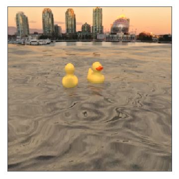
An important consideration in the design of an EDNN was how to choose an appropriate tile size (e.g.
focus and context region). Mills et. al. discusses this process based on the length scale of the physics
of the underlying problem. In the case of counting variable-sized objects present in an image, the
process for choosing a focus and context is less clear. From intuition, we can suggest that the total
tile size (f + 2c) should be large enough to capture an identifiable feature of the largest objects we
wish to count. For example, to count camera-facing waterfowl, one does not need to actually be able
to identify a bird; an accurate count could be obtained by only learning to identify beaks. We found
that using a focus of f = 8 and a context of c = 8 worked well for the MNIST counting purposes.
For the rubber duck counting, we used a slightly larger context, c = 12, as the largest ducks covered
more pixels than the MNIST digits. We will discuss the benefits of different focus and context values
further in the discussion.
With our choice of focus and context, the neural network must be designed to act on tiles of size
(f + 2c) × (f + 2c), 24 × 24 for MNIST and 32 × 32 for the ducks. The input images are zero-padded
with c pixels on all sides, and the tiles are constructed using standard TensorFlow [26] image functions
operating on these zero-padded copies of the input data.
We used a standard convolutional neural network with N = floor(log 2(f + 2c) − 1) layers operating
with K = 64 square kernels of size k = 4. Each layer operated with stride S = 2. The output of the
final convolutional network is flattened and passed into a dense layer with 1024 outputs, which is
then fed into a final dense layer. The final layer has l outputs, where l is the dimensionality of the
labels (i.e. the number of classes being counted).
In practice, the computational graph is constructed to take a batch of N batch L × L images, and
deconstruct them into N tiles = L2 /f 2 tiles. The input data is concatenated along the first axis; this
results in a tensor of shape [N batch × N tiles , f + 2c, f + 2c]. The convolutional neural network
operates on this tensor, performing the same operations on all tiles of all images in the batch, reducing
it to shape [N batch × N tiles , l]. This tensor is then reshaped to [N batch , N tiles , l]; in practice, this
can be thought of “how much stuff” should be attributed to the f × f focus region. We will refer later
to this tensor, so we will label it C. Then for the core of the EDNN technique: a summation reduction
over the second axis. This results in a [N batch , l] tensor denoting the prediction of the l extensive
quantities for each image in the batch. The loss is computed as the mean squared error between this
vector and the vector of labels, and the Adam optimizer [27] is used to minimize this loss.
Standard neural network training procedures were employed using TensorFlow [26] and the Adam
optimizer [27] with a learning rate of 10−4 . We trained the EDNN until the loss dropped below 10−3 ,
between 100 and 500 epochs, depending on the difficulty of the dataset.

3     Results
3.1   MNIST variants

The simplest case is the MNIST-1 dataset. The EDNN is able to count the number of fives with
100.00 % accuracy. Localization of the digits within the input image can be achieved by assigning
the contents of the tile contribution tensor C to the focus regions over which its contributions were
obtained. Doing so results in the ability to detect not only the number of objects in the visual field,
but additionally pinpoint their location with considerable accuracy.
Next is the MNIST-2 dataset, testing the ability of the EDNN to perform mutli-class counting and
localization. The EDNN is tasked with counting 4s and 8s, and does so with 100.00 % accuracy for
both categories. Similarly, localization can be achieved. Interestingly, the EDNN learns to assign
a positive contribution to the class of interest, while assigning a negative contribution to the other
"negative" class. This is because of the EDNN’s limited receptive field; since it only sees a small
region of the input image, in the tiles surrounding a digit, the EDNN cannot see enough information
to identify which class the digit belongs to, and thus assigns a small, positive contribution. Then
when the EDNN sees a tile more central to the negative-class digit, it must output a negative value
to compensate for its misclassification of the exterior regions. The result is still a very precise
localization of each class of objects in the receptive field.
The MNIST-10 dataset includes examples of all ten handwritten digits, from 0 through 9. The EDNN
performs exceptionally well; it performed worst at counting fives, but still performed with 98.08 %
accuracy. The performance of the EDNN on MNIST-10 is shown in Fig. 3.

                                                      4
mnist-1 mnist-2
fives fours
eights
mnist-10
zeros mnist-2-occ
fours
ones
eights
twos
threes mnist-2-occ-vs
fours
fours
eights
fives
sixes rd-1
ducks
sevens
rd-2
eights ducks
nines balls
-1.5 -1.0 -0.5 0.0 0.5 1.0 1.5 -1.5 -1.0 -0.5 0.0 0.5 1.0 1.5
Counting error (true-prediction) Counting error (true-prediction)
(a) (b)
Figure 2: Error distributions for all classes presented in this paper. The minimum, median, and
maximum error for each class is displayed as vertical lines on the distributions. The interval of correct
counting (−0.5 to 0.5) is shaded. A rounding of the final count to integer values would result in any
examples within this interval being counted correctly. We can see easily from these plots that the
MNIST digit counting with occlusion is the most difficult task.
A more difficult challenge is when the digits are permitted to overlap (occlude) other digits. Nonethe-
less, the EDNN is able to count the digits quite accurately with an accuracy of 84.82 % and 88.50 %
for counting fours and eights, respectively.
When variable-sized digits are included in the dataset, and digits are allowed to occlude each other,
the task is considerably more difficult with only 56.68 % and 54.72 % accuracy for counting fours
and eights, respectively. This is not surprising; looking at the example image in Fig. 3, it is difficult
to differentiate many of the digits even by eye.
The error distributions for all datasets are shown in Fig. 2.
3.2 Rubber ducks
Next we move on to the rubber ducks. The EDNN is able to count variable-sized rubber ducks that
are permitted to partially occlude each other, and does so with high accuracy (99.39 %). The dataset
includes five different scenes and a variety of camera angles and lighting conditions affording the
EDNN the opportunity to learn to identify objects and not merely base its prediction on the presence
of a particular colour in the image.
Next we trained an EDNN from scratch on the RD-2 dataset, including multi-colored balls in addition
to the rubber ducks. The EDNN performs exceptionally well, counting the two distinct object classes,
“ducks” and “balls”, with 99.58 % and 99.38 % accuracy, respectively on the test images. An example
is shown in Fig. 3.
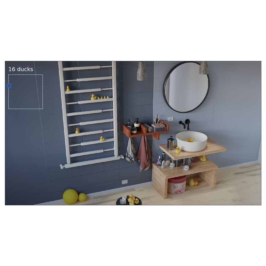
One might question whether the trained model generalizes to rubber ducks which find themselves in
situations not present in the training set. To test this, we construct a 3d-scene of multiple (l0 = 16)
ducks in a bathroom scene [28]. The ducks are various sizes, in various orientations and surrounded
by other 3d objects. The overall image is rendered at a much higher resolution (1920 × 1080) than
5Figure 3: Output of the EDNN for counting and localization of a testing example from three datasets:
MNIST-10, MNIST-2-occ-vs, and RD-2. The top row represents the reference image x. The second
and third rows show the tile contributions C for two of the multi-class labels, e.g. l0 , lN . Red denotes
a large positive contribution, whereas blue denotes a negative contribution. Above, the predicted
object count is displayed (the integral (sum) of C) alongside the true count in parentheses.
6the images present in the training set, however the EDNN technique can easily handle this increase
in size; there are simply more tiles to evaluate prior to the final summation. In fact, EDNN can be
evaluated on arbitrary input sizes so long as the image resolution is a multiple of the focus region
(zero padding can be employed if this is not the case, effectively making this constraint moot). Most
of the ducks in the larger image are of comparable scale to those in the training set. Fig. 4a shows
the scene. The EDNN trained on the duck-only RD-1 dataset does poorly on evaluating the number
of ducks in the bathroom. By looking at C we can form a hypothesis as to why. Summing the
interior of a region of C will tell us how many ducks the EDNN has decided are present within the
boundary of the region. When we do this for some regions-of-interest, we can see that many ducks
are over-counted, while others are under-counted. It is not possible to tell exactly what the problem is,
however the EDNN is clearly considering the yellow balls to be somewhat duck-like. Our best guess
for this failure is that the EDNN is placing too much reliance on the boundary between “yellow” and
“non-yellow” as a good indicator of a duck, and is thus miscounting both large ducks and yellow balls.
If this is indeed the case, the model trained on RD-2 should perform better as the training examples
included yellow balls that the EDNN would have needed to learn are not ducks.
Fig. 4c shows an identical analysis for the model trained on the RD-2 dataset evaluated on the
bathroom scene. The model misses three ducks, but this time the reason is clear: the erroneous counts
are ducks that differ from the ducks in the training set. One duck is significantly smaller than any
ducks present in the training set, and the other two have fallen over, an orientation absent from the
training set.
A remedy for such an issue should be clear; train the EDNN additionally on images of sideways
rubber ducks. This can be accomplished most simply by applying a random rotation by an integer
multiple of π/2 to the input image pipeline during training, augmenting the data set. After doing this,
the EDNN does indeed count the sideways rubber ducks and additionally identifies the tiny duck,
although at a reduced count since it is smaller. Variations in object sizes can also be handled through
data augmentation, scaling down the input images and zero-padding the boundary.
4 Conclusion
We demonstrate the use of an extensive deep neural network for providing multi-class object lo-
calization in images, using weakly-supervised learning. By training an EDNN to count objects in
images, we arrive at a model which can both accurately count instances of objects in images as well
as spatially localize them using only object counts as labels. We demonstrate that multiple classes
of objects can be counted simultaneously (multi-class counting). The EDNN is, through training,
able to develop an internal representation of the objects suitable for counting without any bounding
boxes, point annotations, or ground truth segmentation data. The spatial structure of the EDNN can
be exploited to additionally provide a density map of the objects in the image, providing accurate
localization within the field of view (multi-class localization). Once trained, we demonstrate the
EDNN can be used on images significantly larger and different than those present in the training
dataset. The EDNN technique is a simple and useful technique for computer vision applications.
References
[1] Tobias Stahl, Silvia L Pintea, and Jan C. van Gemert. Divide and Count: Generic Object
Counting by Image Divisions. IEEE Transactions on Image Processing, 28(2):1035–1044, feb
2019.
[2] Alexandra Swanson, Margaret Kosmala, Chris Lintott, Robert Simpson, Arfon Smith, and Craig
Packer. Snapshot Serengeti, high-frequency annotated camera trap images of 40 mammalian
species in an African savanna. Scientific Data, 2:150026, jun 2015.
[3] Kang Han, Wanggen Wan, Haiyan Yao, and Li Hou. Image Crowd Counting Using Convolu-
tional Neural Network and Markov Random Field. pages 1–6, jun 2017.
[4] Yaocong Hu, Huan Chang, Fudong Nian, Yan Wang, and Teng Li. Dense crowd counting from
still images with convolutional neural networks. Journal of Visual Communication and Image
Representation, 38:530–539, 2016.
7b
d
a
c
Figure 4: We used the models trained on the RD-1 and RD-2 datasets to count the number of ducks
in a completely new scene (“bathroom”), at a resolution of 1920 × 1080. We show the scene in
(a), which contains 16 rubber ducks of various sizes. The dashed-line inset in (a) denotes the size
of the training dataset images, 256 × 256 pixels, and a tile is displayed, showing both the focus
(red) and context (blue) regions to scale. In (b) and (c) we overlay the contents of the C tensor,
with some regions highlighted with dashed rectangles. The sums of the interior regions bounded
by the rectangles are printed above, as well as the true number of ducks contained within each
region. Regions containing a correct count (post-rounding) are shown in blue, whereas regions with
an incorrect count are shown in red. In (b), the RD-1 model performs quite poorly, misidentifying
the yellow balls as parts of a duck, and miscounts many regions. In (c), the RD-2 model performs
well, counting most groups of ducks quite accurately. It correctly ignores the yellow balls, as during
training it has seen yellow balls. Three ducks are miscounted; however, these ducks are either in
an orientation or of a size not present in the training set, and thus misidentification is expected. In
(d), we fix this by further training the model on an augmented pipeline with rotations of the original
images included. This results in better overall results, including the fallen ducks and identifying the
tiny duck.
[5] Lingke Zeng, Xiangmin Xu, Bolun Cai, Suo Qiu, and Tong Zhang. Multi-scale convolu-
tional neural networks for crowd counting. Proceedings - International Conference on Image
Processing, ICIP, 2017-Septe:465–469, 2018.
[6] Yingying Zhang, Desen Zhou, Siqin Chen, Shenghua Gao, and Yi Ma. Single-Image Crowd
Counting via Multi-Column Convolutional Neural Network. In 2016 IEEE Conference on
Computer Vision and Pattern Recognition (CVPR), pages 589–597. IEEE, jun 2016.
[7] Cong Zhang, Hongsheng Li, Xiaogang Wang, and Xiaokang Yang. Cross-scene crowd counting
via deep convolutional neural networks. In 2015 IEEE Conference on Computer Vision and
Pattern Recognition (CVPR), pages 833–841. IEEE, jun 2015.
[8] Antoni B. Chan, Zhang-Sheng John Liang, and Nuno Vasconcelos. Privacy preserving crowd
monitoring: Counting people without people models or tracking. In 2008 IEEE Conference on
Computer Vision and Pattern Recognition, pages 1–7. IEEE, jun 2008.
[9] Joseph Paul Cohen, Genevieve Boucher, Craig A. Glastonbury, Henry Z. Lo, and Yoshua Bengio.
Count-ception: Counting by Fully Convolutional Redundant Counting. mar 2017.
[10] Luca Fiaschi ; Ullrich Koethe ; Rahul Nair ; Fred A. Hamprecht. Learning to Count with
Regression Forest and Structured Labels. In Proceedings of the 21st International Conference
on Pattern Recognition (ICPR2012). [IEEE], 2012.
8[11] Antoni B. Chan, Zhang-Sheng John Liang, and Nuno Vasconcelos. Privacy preserving crowd
monitoring: Counting people without people models or tracking. In 2008 IEEE Conference on
Computer Vision and Pattern Recognition, pages 1–7. IEEE, jun 2008.
[12] Elad Walach and Lior Wolf. Learning to Count with CNN Boosting. pages 660–676. Springer,
Cham, 2016.
[13] Weidi Xie, J. Alison Noble, and Andrew Zisserman. Microscopy cell counting and detection with
fully convolutional regression networks. Computer Methods in Biomechanics and Biomedical
Engineering: Imaging & Visualization, 6(3):283–292, may 2018.
[14] Yao Xue, Nilanjan Ray, Judith Hugh, and Gilbert Bigras. Cell Counting by Regression Using
Convolutional Neural Network. pages 274–290. Springer, Cham, 2016.
[15] Alexander Gomez Villa, Augusto Salazar, and Igor Stefanini. Counting Cells in Time-Lapse
Microscopy using Deep Neural Networks. jan 2018.
[16] Mark Marsden, Kevin Mcguinness, Suzanne Little, Ciara E Keogh, and Noel E O’connor.
People, Penguins and Petri Dishes: Adapting Object Counting Models To New Visual Domains
And Object Types Without Forgetting. Technical report, 2017.
[17] Jiyong Chung and Keemin Sohn. Image-Based Learning to Measure Traffic Density Using a
Deep Convolutional Neural Network. IEEE Transactions on Intelligent Transportation Systems,
19(5):1670–1675, may 2018.
[18] Shiv Surya and Venkatesh Babu R. TraCount: a deep convolutional neural network for highly
overlapping vehicle counting. In Proceedings of the Tenth Indian Conference on Computer
Vision, Graphics and Image Processing - ICVGIP ’16, pages 1–6, New York, New York, USA,
2016. ACM Press.
[19] Daniel Oñoro-Rubio and Roberto J López-Sastre. Towards Perspective-Free Object Counting
with Deep Learning. pages 615–629. 2016.
[20] Carlos Arteta, Victor Lempitsky, and Andrew Zisserman. Counting in the Wild. pages 483–498.
Springer, Cham, 2016.
[21] Vishwanath A. Sindagi and Vishal M. Patel. A survey of recent advances in CNN-based single
image crowd counting and density estimation. Pattern Recognition Letters, 107:3–16, 2018.
[22] Jonathan Long, Evan Shelhamer, and Trevor Darrell. Fully Convolutional Networks for Semantic
Segmentation. Technical report, 2016.
[23] Kyle Mills, Kevin Ryczko, Iryna Luchak, Adam Domurad, Chris Beeler, and Isaac Tamblyn.
Extensive deep neural networks for transferring small scale learning to large scale systems.
Chemical Science, 10(15):4129–4140, aug 2019.
[24] Y. Lecun, L. Bottou, Y. Bengio, and P. Haffner. Gradient-based learning applied to document
recognition. Proceedings of the IEEE, 86(11):2278–2324, 1998.
[25] Justin Johnson, Bharath Hariharan, Laurens van der Maaten, Li Fei-Fei, C. Lawrence Zitnick,
and Ross Girshick. CLEVR: A Diagnostic Dataset for Compositional Language and Elementary
Visual Reasoning. dec 2016.
[26] Martín Abadi, Ashish Agarwal, Paul Barham, Eugene Brevdo, Zhifeng Chen, Craig Citro,
Greg S. Corrado, Andy Davis, Jeffrey Dean, Matthieu Devin, Sanjay Ghemawat, Ian Goodfellow,
Andrew Harp, Geoffrey Irving, Michael Isard, Yangqing Jia, Rafal Jozefowicz, Lukasz Kaiser,
Manjunath Kudlur, Josh Levenberg, Dan Mane, Rajat Monga, Sherry Moore, Derek Murray,
Chris Olah, Mike Schuster, Jonathon Shlens, Benoit Steiner, Ilya Sutskever, Kunal Talwar, Paul
Tucker, Vincent Vanhoucke, Vijay Vasudevan, Fernanda Viegas, Oriol Vinyals, Pete Warden,
Martin Wattenberg, Martin Wicke, Yuan Yu, and Xiaoqiang Zheng. TensorFlow: Large-Scale
Machine Learning on Heterogeneous Distributed Systems. None, 1(212):19, mar 2016.
[27] Diederik P. Kingma and Jimmy Ba. Adam: A Method for Stochastic Optimization. pages 1–15,
dec 2014.
[28] Davide Tirindelli. Blue bathroom, 2018.
9You can also read