Active Learning with Partial Feedback
←
→
Page content transcription
If your browser does not render page correctly, please read the page content below
Active Learning with Partial Feedback
                                                       Peiyun Hu1∗, Zachary C. Lipton1,3 , Anima Anandkumar2,3 , Deva Ramanan1
                                                                                         1
                                                                                         Carnegie Mellon University
                                                                                   2
                                                                                       California Institute of Technology
arXiv:1802.07427v3 [cs.LG] 28 Sep 2018

                                                                                                 3
                                                                                                   Amazon AI
                                                      peiyunh@cs.cmu.edu, zlipton@cmu.edu, anima@caltech.edu, deva@cs.cmu.edu

                                                                                             September 27, 2018

                                                                                                       Abstract
                                                      While many active learning papers assume that the learner can simply ask for a label and receive it,
                                                 real annotation often presents a mismatch between the form of a label (say, one among many classes),
                                                 and the form of an annotation (typically yes/no binary feedback). To annotate examples corpora for mul-
                                                 ticlass classification, we might need to ask multiple yes/no questions, exploiting a label hierarchy if one is
                                                 available. To address this more realistic setting, we propose active learning with partial feedback (ALPF),
                                                 where the learner must actively choose both which example to label and which binary question to ask. At
                                                 each step, the learner selects an example, asking if it belongs to a chosen (possibly composite) class. Each
                                                 answer eliminates some classes, leaving the learner with a partial label. The learner may then either ask
                                                 more questions about the same example (until an exact label is uncovered) or move on immediately, leav-
                                                 ing the first example partially labeled. Active learning with partial labels requires (i) a sampling strategy
                                                 to choose (example, class) pairs, and (ii) learning from partial labels between rounds. Experiments on
                                                 Tiny ImageNet demonstrate that our most effective method improves 26% (relative) in top-1 classification
                                                 accuracy compared to i.i.d. baselines and standard active learners given 30% of the annotation budget that
                                                 would be required (naively) to annotate the dataset. Moreover, ALPF-learners fully annotate TinyIma-
                                                 geNet at 42% lower cost. Surprisingly, we observe that accounting for per-example annotation costs can
                                                 alter the conventional wisdom that active learners should solicit labels for hard examples.

                                         1      Introduction
                                         Given a large set of unlabeled images, and a budget to collect annotations, how can we learn an accurate
                                         image classifier most economically? Active Learning (AL) seeks to increase data efficiency by strategically
                                         choosing which examples to annotate. Typically, AL treats the labeling process as atomic: every annotation
                                         costs the same and produces a correct label. However, large-scale multi-class annotation is seldom atomic;
                                         we can’t simply ask a crowd-worker to select one among 1000 classes if they aren’t familiar with our on-
                                         tology. Instead, annotation pipelines typically solicit feedback through simpler mechanisms such as yes/no
                                         questions. For example, to construct the 1000-class ImageNet dataset, researchers first filtered candidates
                                         for each class via Google Image Search, then asking crowd-workers questions like “Is there a Burmese cat
                                             ∗ This   work was done while the author was an intern at Amazon AI

                                                                                                           1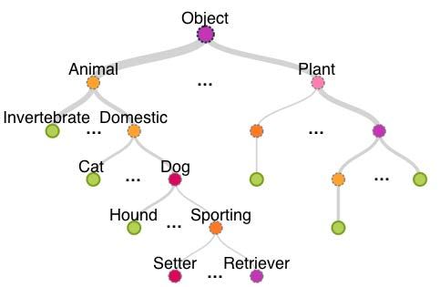
in this image?” (Deng et al., 2009). For tasks where the Google trick won’t work, we might exploit class
hierarchies to drill down to the exact label. Costs scale with the number of questions asked. Thus, real-world
annotation costs can vary per example (Settles, 2011).
We propose Active Learning with Partial Feedback (ALPF), asking, can we cut costs by actively choosing
both which examples to annotate, and which questions to ask? Say that for a new image, our current classifier
places 99% of the predicted probability mass on various dog breeds. Why start at the top of the tree – “is
this an artificial object?” – when we can cut costs by jumping straight to dog breeds (Figure 1)?
ALPF proceeds as follows: In addition to the class
labels, the learner possesses a pre-defined collec-                                                   model

tion of composite classes, e.g. dog ⊃ bulldog, mas-                             training

tiff, .... At each round, the learner selects an (exam-        fully labeled set                                                unlabeled set

ple, class) pair. The annotator responds with binary
feedback, leaving the learner with a partial label. If
only the atomic class label remains, the learner has
                                                              partially labeled set        Does this image contain a dog?    partially labeled set
obtained an exact label. For simplicity, we focus
on hierarchically-organized collections—trees with
atomic classes as leaves and composite classes as
internal nodes.                                                                            Yes

                                                                           Partial feedback                        selected queries
For this to work, we need a hierarchy of concepts                             human
                                                                            annotators
familiar to the annotator. Imagine asking an anno-
tator “is this a foo?” where foo represents a cat-          Figure 1: Workflow for an ALPF learner.
egory comprised of 500 random ImageNet classes.
Determining class membership would be onerous for the same reason that providing an exact label is: It
requires the annotator be familiar with an enormous list of seemingly-unrelated options before answering.
On the other hand, answering “is this an animal?” is easy despite animal being an extremely coarse-grained
category —because most people already know what an animal is.
We use active questions in a few ways. To start, in the simplest setup, we can select samples at random but
then once each sample is selected, choose questions actively until finding the label:

                       ML: “Is it a dog?”                                              Human: Yes!
                       ML: “Is it a poodle?”                                           Human: No!
                       ML: “Is it a hound?”                                            Human: Yes!
                       ML: “Is it a Rhodesian ?”                                       Human: No!
                       ML: “Is it a Dachsund?”                                         Human: Yes!

In ALPF, we go one step further. Since our goal is to produce accurate classifiers on tight budget, should
we necessarily label each example to completion? After each question, ALPF learners have the option of
choosing a different example for the next binary query. Efficient learning under ALPF requires (i) good
strategies for choosing (example, class) pairs, and (ii) techniques for learning from the partially-labeled data
that results when labeling examples to completion isn’t required.
We first demonstrate an effective scheme for learning from partial labels. The predictive distribution is pa-
rameterized by a softmax over all classes. On a per-example basis, we convert the multiclass problem to a
binary classification problem, where the two classes correspond to the subsets of potential and eliminated

                                                          2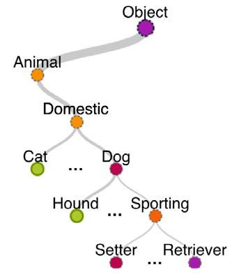
classes. We determine the total probability assigned to potential classes by summing over their softmax
probabilities. For active learning with partial feedback, we introduce several acquisition functions for so-
liciting partial labels, selecting questions among all (example, class) pairs. One natural method, expected
information gain (EIG) generalizes the classic maximum entropy heuristic to the ALPF setting. Our two
other heuristics, EDC and ERC, select based on the number of labels that we expect to see eliminated from
and remaining in a given partial label, respectively.
We evaluate ALPF learners on CIFAR10, CIFAR100, and Tiny ImageNet datasets. In all cases, we use
WordNet to impose a hierarchy on our labels. Each of our experiments simulates rounds of active learning,
starting with a small amount of i.i.d. data to warmstart the models, and proceeding until all examples are
exactly labeled. We compare models by their test-set accuracy after various amounts of annotation. Exper-
iments show that ERC sampling performs best. On TinyImageNet, with a budget of 250k binary questions,
ALPF improves in accuracy by 26% (relative) and 8.1% (absolute) over the i.i.d. baseline. Additionally,
ERC & EDC fully annotate the dataset with just 491k and 484k examples binary questions, respectively (vs
827k), a 42% reduction in annotation cost. Surprisingly, we observe that taking disparate annotation costs
into account may alter the conventional wisdom that active learners should solicit labels for hard examples.
In ALPF, easy examples might yield less information, but are cheaper to annotate.

2    Active Learning with Partial Feedback
By x ∈ Rd and y ∈ Y for Y = {{1}, ..., {k}}, we denote feature vectors and labels. Here d is the feature
dimension and k is the number of atomic classes. By atomic class, we mean that they are indivisible. As in
conventional AL, the agent starts off with an unlabeled training set D = {x1 , ..., xn }.
Composite classes We also consider a pre-specified collection of composite classes C = {c1 , ..., cm }, where
each composite class ci ⊂ {1, ..., k} is a subset of labels such that |ci | ≥ 1. Note that C includes both the
atomic and composite classes. In this paper’s empirical section, we generate composite classes by imposing
an existing lexical hierarchy on the class labels (Miller, 1995).
Partial labels For an example i, we use partial label to describe any element ỹi ⊂ {1, ..., k} such that
ỹi ⊃ yi . We call ỹi a partial label because it may rule out some classes, but doesn’t fully indicate underlying
atomic class. For example, dog = {akita, beagle, bulldog, ...} is a valid partial label when the true label is
{bulldog}. An ALPF learner eliminates classes, obtaining successively smaller partial labels, until only one
(the exact label) remains. To simplify notation, in this paper, by an example’s partial label, we refer to the
smallest partial label available based on the already-eliminated classes. At any step t and for any example i,
           (t)
we use ỹi to denote the current partial label. The initial partial label for every example is ỹ 0 = {1, ..., k}
An exact label is achieved when the partial label ỹi = yi .
Partial Feedback The set of possible questions Q = X × C includes all pairs of examples and composite
classes. An ALPF learner interacts with annotators by choosing questions q ∈ Q. Informally, we pick a
question q = (xi , cj ) and ask the annotator, does xi contain a cj ? If the queried example’s label belongs to
the queried composite class (yi ⊂ cj ), the answer is 1, else 0.
Let αq denote the binary answer to question q ∈ Q. Based on the partial feedback, we can compute the new

                                                        3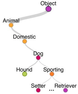
partial label ỹ (t+1) according to Eq. equation 1,
                                                     (t)
                                            (t+1)    ỹ \ c if α = 0
                                         ỹ       =                                                            (1)
                                                     ỹ (t) \ c if α = 1

Note that here ỹ (t) and c are sets, α is a bit, c is a set complement, and that ỹ (t) \ c and ỹ (t) \ c are set
subtractions to eliminate classes from the partial label based on the answer.
Learning Process The learning process is simple: At each round t, the learner selects a pair (x, c) for
labeling. Note that a rational agent will never select either (i) an example for which the exact label is known,
or (ii) a pair (x, c) for which the answer is already known, e.g., if c ⊃ ỹ (t) or c ∩ ỹ (t) = ∅. After receiving
binary feedback, the agent updates the corresponding partial label ỹ (t) → ỹ (t+1) , using Equation 1. The
agent then re-estimates its model, using all available non-trivial partial labels and selects another question q.
In batch-mode, the ALPF learner re-estimates its model once per T queries which is necessary when training
is expensive (e.g. deep learning). We summarize the workflow of a ALPF learner in Algorithm 1.
Objectives We state two goals for ALPF learners. First, we want to learn predictors with low error (on
exactly labeled i.i.d. holdout data), given a fixed annotation budget. Second, we want to fully annotate
datasets at the lowest cost. In our experiments (Section 3), a ALPF strategy dominates on both tasks.

2.1    Learning from partial labels

We now address the task of learning a multiclass classifier from partial labels, a fundamental requirement
of ALPF, regardless of the choice of sampling strategy. At time t, our model ŷ(y, x, θ(t) ) parameterised by
parameters θ(t) estimates the conditional probability of an atomic class y. For simplicity, when the context
is clear, we will use ŷ to designate the full vector of predicted probabilities over all classes. The probability
assigned to a partial  P label ỹ can be expressed by marginalizing over the atomic classes that it contains:
p̂(ỹ (t) , x, θ(t) ) = y∈ỹ(t) ŷ(y, x, θ(t) ). We optimize our model by minimizing the log loss:
                                                      n
                                                   1X       h
                                                                  (t)
                                                                                 i
                                  L(θ(t+1) ) = −         log p̂(ỹi , xi , θ(t) )                              (2)
                                                   n i=1

Note that when every example is exactly labeled, our loss function simplifies to the standard cross entropy
loss often used for multi-class classification. Also note that when every partial label contains the full set of
classes, all partial labels have probability 1 and the update is a no-op. Finally, if the partial label indicates
a composite class such as dog, and the predictive probability mass is exclusively allocated among various
breeds of dog, our loss will be 0. Models are only updated when their predictions disagree (to some degree)
with the current partial label.

2.2    Sampling strategies

Expected Information Gain (EIG): Per classic uncertainty sampling, we can quantify a classifer’s uncer-
tainty via the entropy of the predictive distribution. In AL, each query returns an exact label, and thus the
post-query entropy is always 0. In our case, each answer to the query yields a different partial label. We use

                                                         4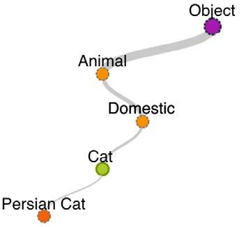
Algorithm 1 Active Learning with Partial Feedback              Table 1: Learning from partial labels on Tiny Ima-
                                                               geNet. These results demonstrate the usefulness of
  Input: X ← (x1 , . . . , xN ), Q ← (q1 , . . . , qM ),
                                                               our training scheme absent the additional complica-
  K, T .
                                                               tions due to ALPF. In each row, γ% of examples are
  Input: D ← [xi ]N               M
                  i=1 , C ← [cj ]j=1 , k, T
               (0)
                                                               assigned labels at the atomic class (Level 0). Levels
  Initialize: ỹi ← {1, . . . , k}, θ ← θ(0) , t ← 0           1, 2, and 4 denote progressively coarser composite
  repeat                                                       labels tracing through the WordNet hierarchy.
    Score every (xi , cj ) with θ
    repeat
                                                                            γ                  (1 − γ)
       Select (xi∗ , cj ∗ ) with the best score                  γ(%)
       Query cj ∗ on data xi∗                                            Level 0    Level 1    Level 2   Level 4
       Receive feedback α                                         20      0.285     +0.113     +0.086     +0.025
                   (t+1)
       Update ỹi∗       according to α                           40      0.351     +0.079     +0.056     +0.016
       t←t+1                                                      60      0.391     +0.051     +0.036     +0.018
                                      (t)
    until (t mod T = 0) or (∀i, |ỹi | = 1)                       80      0.432     +0.015     +0.017     -0.009
    θ ← arg minθ L(θ)
               (t)
  until ∀i, |ỹi | = 1 or t exhausts budget                       100     0.441        -          -          -

the notation ŷ0 , and ŷ1 to denote consequent predictive distributions for each answer (no or yes). We gener-
alize maximum entropy to ALPF by selecting questions with greatest expected reduction in entropy.

                       EIG(x,c) = S(ŷ) − [p̂(c, x, θ)S(ŷ1 ) + (1 − p̂(c, x, θ))S(ŷ0 )]                          (3)

where S(·) is the entropy function. It’s easy to prove that EIG is maximized when p̂(c, x, θ) = 0.5.
Expected Remaining Classes (ERC): Next, we propose ERC, a heuristic that suggests arriving as quickly
as possible at exactly-labeled examples. At each round, ERC selects those examples for which the expected
number of remaining classes is fewest:

                           ERC(x,c) = p̂(c, x, θ)||ŷ1 ||0 + (1 − p̂(c, x, θ))||ŷ0 ||0 ,                          (4)

where ||ŷα || is the size of the partial label following given answer α. ERC is minimized when the result of
the feedback will produce an exact label with probability 1. For a given example xi , if ||ŷi ||0 = 2 containing
only the potential classes (e.g.) dog and cat, then with certainty, ERC will produce an exact label by querying
the class {dog} (or equivalently {cat}). This heuristic is inspired by Cour et al. (2011), which shows that the
partial classification loss (what we optimize with partial labels) is an upper bound of the true classification
                                                                1
loss (as if true labels are available) with a linear factor of 1−ε , where ε is ambiguity degree and ε ∝ |ỹ|. By
selecting q ∈ Q that leads to the smallest |ỹ|, we can tighten the bound to make optimization with partial
labels more effective.
Expected Decrease in Classes (EDC): More in keeping with the traditional goal of minimizing uncertainty,
we might choose EDC, the sampling strategy which we expect to result in the greatest reduction in the
number of potential classes. We can express EDC as the difference between the number of potential labels
(known) and the expected number of potential labels remaining: EDC(x,c) = |ỹ (t) | − ERC(x,c) .

                                                           5
3 Experiments
We evaluate ALPF algorithms on the CIFAR10, CIFAR100, and Tiny ImageNet datasets, with training sets
of 50k, 50k, and 100k examples, and 10, 100, and 200 classes respectively. After imposing the Wordnet
hierarchy on the label names, the size of the set of possible binary questions |C| for each dataset are 27,
261, and 304, respectively. The number of binary questions between re-trainings are 5k, 15k, and 30k,
respectively. By default, we warm-start each learner with the same 5% of training examples selected i.i.d.
and exactly labeled. Warm-starting has proven essential in other papers combining deep and active learning
(Shen et al., 2018). Our own analysis (Section 3.3) confirms the importance of warm-starting although the
affect appears variable across acquisition strategies.
Model For each experiment, we adopt the widely-popular ResNet-18 architecture (He et al., 2016). Because
we are focused on active learning and thus seek fundamental understanding of this new problem formulation,
we do not complicate the picture with any fine-tuning techniques. Note that some leaderboard scores circu-
lating on the Internet appear to have far superior numbers. This owes to pre-training on the full ImageNet
dataset (from which Tiny-ImageNet was subsampled and downsampled), constituting a target leak.
We initialize weights with the Xavier technique (Glorot and Bengio, 2010) and minimize our loss using
the Adam (Kingma and Ba, 2014) optimizer, finding that it outperforms SGD significantly when learning
from partial labels. We use the same learning rate of 0.001 for all experiments, first-order momentum decay
(β1 ) of 0.9, and second-order momentum decay (β2 ) of 0.999. Finally, we train with mini-batches of 200
examples and perform standard data augmentation techniques including random cropping, resizing, and
mirror-flipping. We implement all models in MXNet and have posted our code publicly1 .
Re-training Ideally, we might update models after each query, but this is too costly. Instead, following
Shen et al. (2018) and others, we alternately query labels and update our models in rounds. We warm-start
all experiments with 5% labeled data and iterate until every example is exactly labeled. At each round, we
re-train our classifier from scratch with random initialization. While we could initialize the new classifier
with the previous best one (as in Shen et al. (2018)), preliminary experiments showed that this faster con-
vergence comes at the cost of worse performance, perhaps owing to severe over-fitting to labels acquired
early in training. In all experiments, for simplicity, we terminate the optimization after 75 epochs. Since
30k questions per re-training (for TinyImagenet) seems infrequent, we compared against 10x more frequent
re-training More frequent training conferred no benefit (Appendix B).
3.1 Learning from partial labels
Since the success of ALPF depends in part on learning from partial labels, we first demonstrate the efficacy
of learning from partial labels with our loss function when the partial labels are given a priori. In these
experiments we simulate a partially labeled dataset and show that the learner achieves significantly better
accuracy when learning from partial labels than if it excluded the partial labels and focused only on exactly
annotated examples. Using our WordNet-derived hierarchy, we conduct experiments with partial labels at
different levels of granularity. Using partial labels from one level above the leaf, German shepherd becomes
dog. Going up two levels, it becomes animal.
We first train a standard multi-class classifier with γ (%) exactly labeled training data and then another
classifier with the remaining (1 − γ)% partially labeled at a different granularity (level of hierarchy). We
1 Our implementations of ALPF learners are available at: https://github.com/peiyunh/alpf
60.5 1.0 200
Baseline
AQ - EIG
175 AQ - EDC
0.4 0.8 AQ - ERC
150 ALPF - EIG
pct. of exactly labeled examples
ALPF - EDC
num. of remaining classes
ALPF - ERC
0.3 0.6 125
top1 acc.
100
Baseline
0.2 AL - ME 0.4 75
AL - LC Baseline
AQ - EIG AQ - EIG
AQ - EDC AQ - EDC 50
0.1 AQ - ERC 0.2 AQ - ERC
ALPF - EIG ALPF - EIG 25
ALPF - EDC ALPF - EDC
ALPF - ERC ALPF - ERC
0.0 0.0 0
0 200 400 600 800 1000 0 200 400 600 800 1000 0 200 400 600 800 1000
num. of questions (1000s) num. of questions (1000s) num. of questions (1000s)
Figure 2: The progression of top1 classification accuracy (left), percentage of exactly labeled training exam-
ples (middle), and average number of remaining classes (right).
compare the classifier performance on holdout data both with and without adding partial labels in Table 1.
We make two key observations: (i) additional coarse-grained partial labels improve model accuracy (ii) as
expected, the improvement diminishes as partial label gets coarser. These observations suggest we can learn
effectively given a mix of exact and partial labels.
3.2 Sampling strategies
Baseline This learner samples examples at random. Once an example is sampled, the learner applies top-
down binary splitting—choosing the question that most evenly splits the probability mass, see Related Work
for details— with a uniform prior over the classes until that example is exactly labeled.
AL To disentangle the effect of active sampling of questions and samples, we compare to conventional AL
approaches selecting examples with uncertainty sampling but selecting questions as baseline.
AQ Active questions learners, choose examples at random but use partial feedback strategies to efficiently
label those examples, moving on to the next example after finding an example’s exact label.
ALPF ALPF learners are free to choose any (example, question) pair at each turn, Thus, unlike AL and AQ,
ALPF learners commonly encounter partial labels during training.
Results We run all experiments until fully annotating the training set. We then evaluate each method from
two perspectives: classification and annotation. We measure each classifiers’ top-1 accuracy at each an-
notation budget. To quantify annotation performance, we count the number questions required to exactly
label all training examples. We compile our results in Table 2, rounding costs to 10%, 20% etc. The budget
includes the (5%) i.i.d. data for warm-starting. Some key results: (i) vanilla active learning does not im-
prove over i.i.d. baselines, confirming similar observations on image classification by Sener and Savarese
(2017); (ii) AQ provides a dramatic improvement over baseline. The advantage persists throughout training.
These learners sample examples randomly and label to completion (until an exact label is produced) before
moving on, differing only in how efficiently they annotate data. (iii) On Tiny ImageNet, at 30% of budget,
ALPF-ERC outperforms AQ methods by 4.5% and outperforms the i.i.d. baseline by 8.1%.
7EIG EIG
6 1.0 1.0
ALPF - EIG
ALPF - EDC 0.5 0.5
5 ALPF - ERC
attacked real label distribution
normal real label distribution
0.0 EDC 0.0 EDC
1.0 1.0
4
0.5 0.5
entropy (bits)
3
0.0 ERC 0.0 ERC
1.0 1.0
2
0.5 0.5
1 0.0 0.0
0 5 10 15 20 25 0 5 10 15 20 25
round of annotation round of annotation
0
0 100 200 300 400 500 600
num. of questions (1000s) (a) Normal CIFAR10 (b) Adversarial CIFAR10
Figure 3: Classifier confi- Figure 4: Label distribution among selected examples for CIFAR 10
dence (entropy of softmax (left) and adversarially perturbed CIFAR 10 (right). Light green and
layer) on selected examples. light purple mark the two classes made artificially easy.
3.3 Diagnostic analyses
First, we study how different amounts of warm-starting affects ALPF learners’ performance with a small
set of i.i.d. labels. Second, we compare the selections due to ERC and EDC to those produced through
uncertainty sampling. Third, we note that while EDC and ERC appear to perform best on our problems,
they may be vulnerable to excessively focusing on classes that are trivial to recognize. We examine this
setting via an adversarial dataset intended to break the heuristics.
Warm-starting We compare the performance of each strategy under different percentages (0%, 5%, and
10%) of pre-labeled i.i.d. data (Figure 5, Appendix A). Results show that ERC works properly even without
warm-starting, while EIG benefits from a 5% warm-start and EDC suffers badly without warm-starting. We
observe that 10% warm-starting yields no further improvement.
Sample uncertainty Classic uncertainty sampling chooses data of high uncertainty. This question is worth
re-examining in the context of ALPF. To analyze the behavior of ALPF learners vis-a-vis uncertainty we
plot average prediction entropy of sampled data for ALPF learners with different sampling strategies (Fig-
ure 3). Note that ALPF learners using EIG pick high-entropy data, while ALPF learners with EDC and
ERC choose examples with lower entropy predictions. The (perhaps) surprising performance of EDC and
ERC may owe to the cost structure of ALPF. While labels for examples with low-entropy predictions confer
less information, they also come at lower cost.
Adversarial setting Because ERC goes after “easy” examples, we test its behavior on a simulated dataset
where 2 of the CIFAR10 classes (randomly chosen) are trivially easy. We set all pixels white for one class
all pixels black for the other. We plot the label distribution among the selected data over rounds of selection
in against that on the unperturbed CIFAR10 in Figure 4. As we can see, in the normal case, EIG splits its
budget among all classes roughly evenly while EDC and ERC focus more on different classes at different
stages. In the adversarial case, EIG quickly learns the easy classes, thereafter focusing on the others until
they are exhausted, while EDC and ERC concentrate on exhausting the easy ones first. Although EDC and
ERC still manage to label all data with less total cost than EIG, this behavior might cost us when we have
trivial classes, especially when our unlabeled dataset is enormous relative to our budget.
84 Related work
Binary identification: Efficiently finding answers with yes/no questions is a classic problem (Garey, 1972)
dubbed binary identification. Hyafil and Rivest (1976) proved that finding the optimal strategy given an
arbitrary set of binary tests is NP-complete. A well-known greedy algorithm called binary splitting (Garey
and Graham, 1974; Loveland, 1985), chooses questions that most evenly split the probability mass.
Active learning: Our work builds upon the AL framework (Box and Draper, 1987; Cohn et al., 1996;
Settles, 2010) (vs. i.i.d labeling). Classical AL methods select examples for which the current predictor is
most uncertain, according to various notions of uncertainty: Dagan and Engelson (1995) selects examples
with maximum entropy (ME) predictive distributions, while Culotta and McCallum (2005) uses the least
confidence (LC) heuristic, sorting examples in ascending order by the probability assigned to the argmax.
Settles et al. (2008) notes that annotation costs may vary across data points suggesting cost-aware sampling
heuristics but doesn’t address the setting when costs change dynamically during training as a classifier
grows stronger. Luo et al. (2013) incorporates structure among outputs into an active learning scheme in the
context of structured prediction. Mo et al. (2016) addresses hierarchical label structure in active learning
interestingly in a setting where subclasses are easier to learn. Thus they query classes more fine-grained
than the targets, while we solicit feedback on more general categories.
Deep Active Learning Deep Active Learning (DAL) has recently emerged as an active research area. Wang
et al. (2016) explores a scheme that combines traditional heuristics with pseudo-labeling. Gal et al. (2017)
notes that the softmax outputs of neural networks do not capture epistemic uncertainty (Kendall and Gal,
2017), proposing instead to use Monte Carlo samples from a dropout-regularized neural network to produce
uncertainty estimates. DAL has demonstrated success on NLP tasks. Zhang et al. (2017) explores AL for
sentiment classification, proposing a new sampling heuristic, choosing examples for which the expected
update to the word embeddings is largest. Recently, Shen et al. (2018) matched state of the art performance
on named entity recognition, using just 25% of the training data. Kampffmeyer et al. (2016) and Kendall
et al. (2015) explore other measures of uncertainty over neural network predictions.
Learning from partial labels Many papers on learning from partial labels (Grandvalet and Bengio, 2004;
Nguyen and Caruana, 2008; Cour et al., 2011) assume that partial labels are given a priori and fixed. Grand-
valet and Bengio (2004) formalizes the partial labeling problem in the probabilistic framework and proposes
a minimum entropy based solution. Nguyen and Caruana (2008) proposes an efficient algorithm to learn
classifiers from partial labels within the max-margin framework. Cour et al. (2011) addresses desirable
properties of partial labels that allow learning from them effectively. While these papers assume a fixed set
of partial labels, we actively solicit partial feedback. This presents new algorithmic challenges: (i) the partial
labels for each data point changes across training rounds; (ii) the partial labels result from active selection,
which introduces bias; and (iii) our problem setup requires a sampling strategy to choose questions.
5 Conclusion
Our experiments validate the active learning with partial feedback framework on large-scale classification
benchmarks. The best among our proposed ALPF learners fully labels the data with 42% fewer binary
questions as compared to traditional active learners. Our diagnostic analysis suggests that in ALPF, it’s
sometimes more efficient to start with “easier” examples that can be cheaply annotated rather than with
“harder” data as often suggested by traditional active learning.
9Table 2: Results on Tiny ImageNet (N/A indicates data has been fully labeled)
Annotation Budget Labeling Cost
(w.r.t. baseline labeling cost)
10% 20% 30% 40% 50% 100%
TinyImageNet
Baseline 0.186 0.266 0.310 0.351 0.354 0.441 827k
AL - ME 0.169 0.269 0.303 0.347 0.365 - 827k
AL - LC 0.184 0.262 0.313 0.355 0.369 - 827k
AQ - EIG 0.186 0.283 0.336 0.381 0.393 - 545k
AQ - EDC 0.196 0.291 0.353 0.386 0.415 - 530k
AQ - ERC 0.194 0.295 0.346 0.394 0.406 - 531k
ALPF - EIG 0.203 0.289 0.351 0.384 0.420 - 575k
ALPF - EDC 0.220 0.319 0.363 0.397 0.420 - 482k
ALPF - ERC 0.207 0.330 0.391 0.419 0.427 - 491k
CIFAR100
Baseline 0.252 0.340 0.412 0.437 0.469 0.537 337k
AL - ME 0.237 0.321 0.388 0.419 0.458 - 337k
AL - LC 0.247 0.332 0.398 0.432 0.468 - 337k
AQ - EIG 0.266 0.354 0.443 0.485 0.502 - 208k
AQ - EDC 0.264 0.366 0.439 0.483 0.508 - 215k
AQ - ERC 0.256 0.366 0.453 0.479 0.496 - 215k
ALPF - EIG 0.263 0.341 0.423 0.466 0.497 - 235k
ALPF - EDC 0.281 0.367 0.442 0.479 0.518 - 193k
ALPF - ERC 0.273 0.379 0.464 0.502 0.526 - 187k
CIFAR10
Baseline 0.645 0.718 0.757 0.778 0.792 0.829 170k
AL - ME 0.663 0.709 0.759 0.763 0.800 - 170k
AL - LC 0.644 0.724 0.753 0.780 0.792 - 170k
AQ - EIG 0.654 0.747 0.791 0.806 0.823 - 89k
AQ - EDC 0.675 0.746 0.784 0.789 0.826 - 95k
AQ - ERC 0.682 0.750 0.771 0.811 0.822 - 96k
ALPF - EIG 0.673 0.741 0.786 0.815 0.813 - 124k
ALPF - EDC 0.676 0.752 0.797 0.832 N/A - 74k
ALPF - ERC 0.670 0.743 0.797 0.833 N/A - 74k
10References
Box, G. E. and Draper, N. R. (1987). Empirical model-building and response surfaces. John Wiley & Sons.
Cohn, D. A., Ghahramani, Z., and Jordan, M. I. (1996). Active learning with statistical models. Journal of
artificial intelligence research (JAIR).
Cour, T., Sapp, B., and Taskar, B. (2011). Learning from partial labels. Journal of Machine Learning
Research, 12(May):1501–1536.
Culotta, A. and McCallum, A. (2005). Reducing labeling effort for structured prediction tasks.
Dagan, I. and Engelson, S. P. (1995). Committee-based sampling for training probabilistic classifiers.
Deng, J., Dong, W., Socher, R., Li, L.-J., Li, K., and Fei-Fei, L. (2009). Imagenet: A large-scale hierarchical
image database. In Computer Vision and Pattern Recognition (CVPR).
Gal, Y., Islam, R., and Ghahramani, Z. (2017). Deep bayesian active learning with image data.
arXiv:1703.02910.
Garey, M. R. (1972). Optimal binary identification procedures. SIAM Journal on Applied Mathematics.
Garey, M. R. and Graham, R. L. (1974). Performance bounds on the splitting algorithm for binary testing.
Acta Informatica.
Glorot, X. and Bengio, Y. (2010). Understanding the difficulty of training deep feedforward neural networks.
In Artificial Intelligence and Statistics (AISTATS).
Grandvalet, Y. and Bengio, Y. (2004). Learning from partial labels with minimum entropy.
He, K., Zhang, X., Ren, S., and Sun, J. (2016). Deep residual learning for image recognition. In Computer
Vision and Pattern Recognition (CVPR).
Hyafil, L. and Rivest, R. L. (1976). Constructing optimal binary decision trees is np-complete. Information
processing letters.
Kampffmeyer, M., Salberg, A.-B., and Jenssen, R. (2016). Semantic segmentation of small objects and
modeling of uncertainty in urban remote sensing images using deep convolutional neural networks. In
CVPR.
Kendall, A., Badrinarayanan, V., and Cipolla, R. (2015). Bayesian segnet: Model uncertainty in deep
convolutional encoder-decoder architectures for scene understanding. arXiv:1511.02680.
Kendall, A. and Gal, Y. (2017). What uncertainties do we need in bayesian deep learning for computer
vision? In NIPS.
Kingma, D. and Ba, J. (2014). Adam: A method for stochastic optimization. In International Conference
on Learning Representations (ICLR).
Loveland, D. W. (1985). Performance bounds for binary testing with arbitrary weights. Acta Informatica.
Luo, W., Schwing, A., and Urtasun, R. (2013). Latent structured active learning. In Advances in Neural
Information Processing Systems (NIPS).
Miller, G. A. (1995). Wordnet: a lexical database for english. Communications of the ACM.
11Mo, Y., Scott, S. D., and Downey, D. (2016). Learning hierarchically decomposable concepts with active
over-labeling. In International Conference on Data Mining (ICDM).
Nguyen, N. and Caruana, R. (2008). Classification with partial labels. In Knowledge discovery and data
mining (KDD). ACM.
Sener, O. and Savarese, S. (2017). Active learning for convolutional neural networks: a core-set approach.
In ICLR.
Settles, B. (2010). Active learning literature survey. University of Wisconsin, Madison, 52(55-66):11.
Settles, B. (2011). From theories to queries: Active learning in practice. In Active Learning and Experimen-
tal Design workshop In conjunction with AISTATS 2010, pages 1–18.
Settles, B., Craven, M., and Friedland, L. (2008). Active learning with real annotation costs.
Shen, Y., Yun, H., Lipton, Z. C., Kronrod, Y., and Anandkumar, A. (2018). Deep active learning for named
entity recognition. In ICLR.
Wang, K., Zhang, D., Li, Y., Zhang, R., and Lin, L. (2016). Cost-effective active learning for deep image
classification. IEEE Transactions on Circuits and Systems for Video Technology.
Zhang, Y., Lease, M., and Wallace, B. C. (2017). Active discriminative text representation learning.
12A Warm-starting Plot
Figure 5 compares our strategies under various amounts of warm-starting with pre-labeled i.i.d. data.
0.5 0.5 0.5
0.4 0.4 0.4
0.3 0.3 0.3
top1 acc.
top1 acc.
top1 acc.
0.2 0.2 0.2
0.1 ALPF - EIG - 0% 0.1 ALPF - EDC - 0% 0.1 ALPF - ERC - 0%
ALPF - EIG - 5% ALPF - EDC - 5% ALPF - ERC - 5%
ALPF - EIG - 10% ALPF - EDC - 10% ALPF - ERC - 10%
0.0 0.0 0.0
0 200 400 600 800 1000 0 200 400 600 800 1000 0 200 400 600 800 1000
num. of questions (1000s) num. of questions (1000s) num. of questions (1000s)
Figure 5: This plot compares our models under various amounts of warm-starting with pre-labeled i.i.d.
data. We find that on the investigated datasets, ERC does benefit from warm-starting. However, absent
warm-starting, EIG performs significantly worse and EDC suffers even more. We find that 5% warmstarting
helps these two models and that for both, increasing warm-starting from 5% up to 10% does not lead to
further improvements.
B Updating models more frequently
On Tiny ImageNet, we normally re-initialize and train models from scratch for 75 epochs after every 30K
questions. Since we found re-initialization is crucial for good performance, to ensure a fair comparison, we
keep the same re-initialization frequency (i.e. every 30K questions) while updating the model by fine-tuning
5 epochs after every 3K questions. This results in 10X faster model updating frequency. As in Figure 6
and Table 3, results show only ALPF-EDC and ALPF-ERC seem to benefit from updating 10 times more
frequently
13Table 3: Updating models after every 30K questions (1X) vs. after every 3K (10X)
Annotation Budget Labeling Cost
10% 20% 30% 40% 50% 100%
TinyImageNet
Baseline 0.186 0.266 0.310 0.351 0.354 0.441 827k
AL - ME 0.169 0.269 0.303 0.347 0.365 - 827k
AL - LC 0.184 0.262 0.313 0.355 0.369 - 827k
AL - ME - 10X 0.177 0.260 0.304 0.341 0.359 -
AL - LC - 10X 0.188 0.257 0.308 0.347 0.369 -
AQ - EIG 0.186 0.283 0.336 0.381 0.393 - 545k
AQ - EDC 0.196 0.291 0.353 0.386 0.415 - 530k
AQ - ERC 0.194 0.295 0.346 0.394 0.406 - 531k
AQ - EIG - 10X 0.200 0.284 0.349 0.379 0.402 - 522k
AQ - EDC - 10X 0.186 0.294 0.326 0.383 0.408 - 522k
AQ - ERC - 10X 0.201 0.292 0.338 0.383 0.407 - 522k
ALPF - EIG 0.203 0.289 0.351 0.384 0.420 - 575k
ALPF - EDC 0.220 0.319 0.363 0.397 0.420 - 482k
ALPF - ERC 0.207 0.330 0.391 0.419 0.427 - 491k
ALPF - EIG - 10X 0.199 0.293 0.352 0.391 0.406 - 581k
ALPF - EDC - 10X 0.231 0.352 0.387 0.410 0.409 - 521k
ALPF - ERC - 10X 0.235 0.342 0.382 0.417 0.426 - 521k
14Baseline
0.45 Uniform (1X)
Uniform (10X)
0.40
0.35
top1 acc.
0.30
0.25
0.20
0.15
100 200 300 400 500 600 700 800
num. of questions (1000s)
AD - (ME, LC)
0.45 AL_ME (1X) 0.45 AL_LC (1X)
AL_ME (10X) AL_LC (10X)
0.40 0.40
0.35 0.35
0.30
top1 acc.
top1 acc.
0.30
0.25 0.25
0.20 0.20
0.15 0.15
100 200 300 400 500 600 700 800 100 200 300 400 500 600 700 800
num. of questions (1000s) num. of questions (1000s)
AQ - (EIG, EDC, ERC)
0.45 AQ_EIG (1X) 0.45 AQ_EDC (1X) 0.45 AQ_ERC (1X)
AQ_EIG (10X) AQ_EDC (10X) AQ_ERC (10X)
0.40 0.40 0.40
0.35 0.35 0.35
0.30 0.30 0.30
top1 acc.
top1 acc.
top1 acc.
0.25 0.25 0.25
0.20 0.20 0.20
0.15 0.15 0.15
100 200 300 400 500 100 200 300 400 500 100 200 300 400 500
num. of questions (1000s) num. of questions (1000s) num. of questions (1000s)
ALPF - (EIG, EDC, ERC)
0.45 ALPF_EIG (1X) 0.45 ALPF_EDC (1X) 0.45 ALPF_ERC (1X)
ALPF_EIG (10X) ALPF_EDC (10X) ALPF_ERC (10X)
0.40 0.40 0.40
0.35 0.35 0.35
top1 acc.
top1 acc.
top1 acc.
0.30 0.30 0.30
0.25 0.25 0.25
0.20 0.20 0.20
0.15 0.15 0.15
15
100 200 300 400 500 600 100 200 300 400 500 100 200 300 400 500
num. of questions (1000s) num. of questions (1000s) num. of questions (1000s)
Figure 6: Updating models after every 30K questions (1X) vs. after every 3K (10X)You can also read