Quantitative imaging and automated fuel pin identification for passive gamma emission tomography
←
→
Page content transcription
If your browser does not render page correctly, please read the page content below
www.nature.com/scientificreports
OPEN Quantitative imaging
and automated fuel pin
identification for passive gamma
emission tomography
Ming Fang1*, Yoann Altmann2, Daniele Della Latta3,4, Massimiliano Salvatori3,5 &
Angela Di Fulvio1
Compliance of member States to the Treaty on the Non-Proliferation of Nuclear Weapons is monitored
through nuclear safeguards. The Passive Gamma Emission Tomography (PGET) system is a novel
instrument developed within the framework of the International Atomic Energy Agency (IAEA) project
JNT 1510, which included the European Commission, Finland, Hungary and Sweden. The PGET is
used for the verification of spent nuclear fuel stored in water pools. Advanced image reconstruction
techniques are crucial for obtaining high-quality cross-sectional images of the spent-fuel bundle
to allow inspectors of the IAEA to monitor nuclear material and promptly identify its diversion.
In this work, we have developed a software suite to accurately reconstruct the spent-fuel cross
sectional image, automatically identify present fuel rods, and estimate their activity. Unique image
reconstruction challenges are posed by the measurement of spent fuel, due to its high activity and
the self-attenuation. While the former is mitigated by detector physical collimation, we implemented
a linear forward model to model the detector responses to the fuel rods inside the PGET, to account
for the latter. The image reconstruction is performed by solving a regularized linear inverse problem
using the fast-iterative shrinkage-thresholding algorithm. We have also implemented the traditional
filtered back projection (FBP) method based on the inverse Radon transform for comparison and
applied both methods to reconstruct images of simulated mockup fuel assemblies. Higher image
resolution and fewer reconstruction artifacts were obtained with the inverse-problem approach, with
the mean-square-error reduced by 50%, and the structural-similarity improved by 200%. We then used
a convolutional neural network (CNN) to automatically identify the bundle type and extract the pin
locations from the images; the estimated activity levels finally being compared with the ground truth.
The proposed computational methods accurately estimated the activity levels of the present pins,
with an associated uncertainty of approximately 5%.
Under the Treaty on the Non-Proliferation of Nuclear Weapons (NPT)1 and other treaties against nuclear pro-
liferation, the International Atomic Energy Agency (IAEA) is entrusted to verify all nuclear materials under the
control of the State with safeguards agreements in force with the Agency. International safeguards include all the
technical measures put in place by the IAEA to verify that each State Parties complies with the aforementioned
agreements.
Most safeguards methods are based on the assay of nuclear materials through measurements of ionizing
radiation emitted by the sample. Safeguards systems are undergoing an important modernization e ffort2. One
example of such effort is the development of the PGET systems for the inspection of spent fuel in water pools3–5.
Traditionally, an inspection of spent fuel in pools was performed using the FORK detector, which encompasses,
in its standard version, one ionization chamber to measure gamma rays and two neutron-sensitive fission cham-
bers. The FORK detector, however, exhibits low sensitivity to the diversion of fuel pins, being able to detect the
diversion of 50% or more of the fuel pins in the assembly under inspection6. A PGET was recently developed
1
Department of Nuclear, Plasma, and Radiological Engineering, University of Illinois at Urbana-Champaign,
Urbana, IL 61801, US. 2School of Engineering and Physical Sciences, Heriot-Watt University, Riccarton,
Edinburgh EH14 4AS, UK. 3Fondazione Toscana Gabriele Monasterio, Via Giuseppe Moruzzi, 1, 56124 Pisa, PI,
Italy. 4Present address: Terarecon Inc., 4309 Emperor Blvd, Suite 310, Durham, NC 27703, US. 5Present address:
Kymamed Srls, Viale Roma 208, 54100 Massa, Italy. *email: mingf2@illinois.edu
Scientific Reports | (2021) 11:2442 | https://doi.org/10.1038/s41598-021-82031-8 1
Vol.:(0123456789)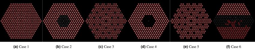
www.nature.com/scientificreports/
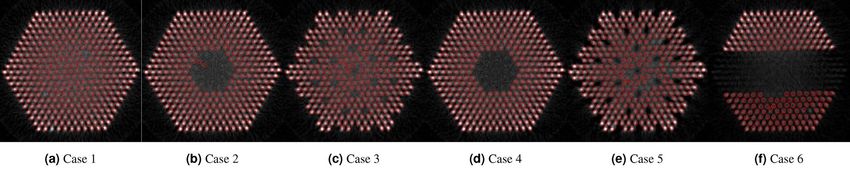
Figure 1. Actual pin distributions in the simulated fuel assemblies (ground truth). Pin activity is proportional
to the brightness. In Case 1, the mock-up fuel assembly hosted 331 60Co pins of 8.879 g/cm3 density, which
emitted 1.17 and 1.33 MeV gamma rays. In Cases 2 and 3, 10% 60Co pins pins were removed at the center or
uniformly. In Cases 4 and 5, 10% 60Co pins pins were replaced by depleted uranium pins of the same size but
higher density (10.4 g/cm3 ). In Case 6, we decreased the activities of the middle pins by 80% and bottom pins by
50%.
15000
150
10000
Detector
100
50 5000
0
0 50 100 150 200 250 300 350
Angle (degree)
Figure 2. Simulated sinogram of the fully-loaded bundle. The color scale represents the detected photon
counts. The periodicity of the singogram resulted from the hexagonal symmetry of the simulated fuel assembly.
to increase the sensitivity to a variety of fuel diversion s cenarios5. The software to analyze PGET images can be
improved7 to reduce user intervention and overall perform faster and more reliable monitoring of spent fuel and
therefore implement the ultimate safeguards objective, i.e., the prompt detection of nuclear material diverted
from peaceful uses.
The PGET of spent fuel poses some unique challenges, compared to industrial or medical tomographic imag-
ing, which are due to the high activity of the sources (a single-pin activity is of the order of 1013 Bq) and the high
self-attenuation of the fuel pins. While the former can be mitigated using collimated detectors, the latter needs
to be addressed by using specific imaging algorithms. Previous work has shown that the reconstruction quality
could be significantly improved by applying the attenuation c orrection8. In this work, we further corrected for
the gamma ray down-scattering in the energy window of interest. We have implemented and integrated compu-
tational methods based on proximal gradient, physics-informed Monte Carlo sampling, and machine learning to
(1) improve the PGET image quality, (2) automatically identify missing pins, and (3) quantify the pin activities.
As we will show, the automated identification of missing pins relies heavily on the image quality, and therefore
the three tasks are inherently intertwined.
Results
Simulated sinograms. We simulated the measurement of six fuel pin configurations in a mock-up water-
water energetic reactor (VVER) fuel assembly using MCNP 6.29, as shown in Fig. 1. In Cases 2 and 3, we mim-
icked the scenario where fuel pins were missing. In Cases 4 and 5, we used depleted uranium to replace cobalt
because it resulted in the highest attenuation among different potential replacement m aterials10, which would
allow us to examine the algorithm’s capability of distinguishing replaced pins. In Case 6, we wanted to explore
whether the algorithm is able to render an accurate image of a space-dependent activity distribution. Details of
the simulated PGET model are included in “Methods-Simulation Methods" section.
The detection system we simulated is the so-called PGET prototype device as described b y4. The detection
unit consisted of two collimated CdTe detector arrays on opposite sides of the fuel assembly, each encompassing
91 detectors. The detector arrays rotated and scanned the fuel bundle in steps of 1◦, which generated a 182 × 360
sinogram, as shown in Fig. 2. We simulated 5 × 10⁹ NPS (number of particle histories) in each case and detected
the photons in the 700-1500 keV energy window. Approximately 15,000 maximum counts in one pixel were
achieved, comparable to the counts in an actual PGET measurement.
Inverse approach. We have developed a systematic approach that allows us to reconstruct high-quality
images from individual sinograms, identify the pin locations, and quantify the pin activity levels. The image of
fuel pins was reconstructed by solving a linear inverse problem. The region of interest was divided into 182 × 182
Scientific Reports | (2021) 11:2442 | https://doi.org/10.1038/s41598-021-82031-8 2
Vol:.(1234567890)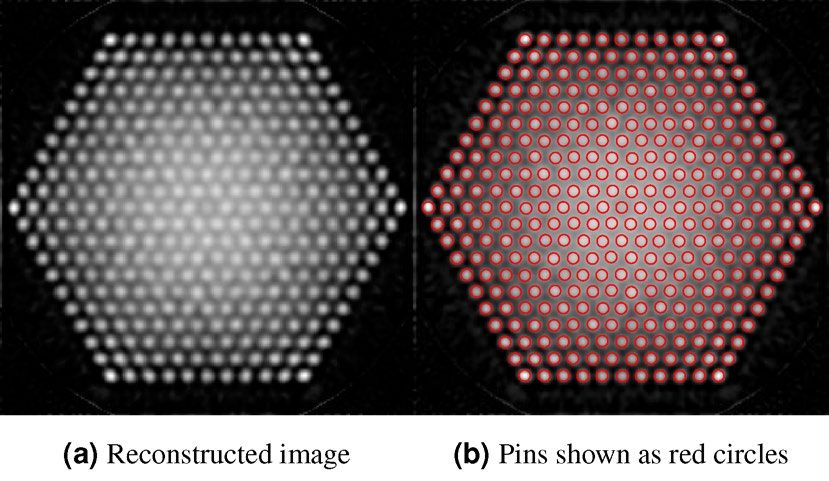
www.nature.com/scientificreports/
Figure 3. Image reconstruction and pin identification using the simple response matrix in Case 1.
50 y = 41.89 exp(−4.69(x − 0.59)2)
Line profile
40
Pixel value
30
FWHM
20
10
0.0 0.5 1.0
x (cm)
Figure 4. Gaussian fit of the average line profile. FWHM of the fitted Gaussian is shown as the arrow. The 11
pixels around the pin center shown as the red points were used in the fitting. The coefficient of determination R2
of the fit was 0.9991.
pixels. We calculated the detector array response to a source of unit activity inside each pixel, forming the system
response matrix. For an unknown fuel assembly, the measured sinogram is a linear combination of the calcu-
lated responses, with the coefficients being the source strength of each pixel. In this way, the image reconstruc-
tion problem was converted into a linear inverse problem, with both the simulated sinogram and calculated
response matrix as inputs.
First, we performed a simple image reconstruction to obtain an initial estimate of pin locations and pin
radius. We calculated the system response matrix using a deterministic ray-tracing method, assuming that the
scattering of gamma rays can be n eglected11. The reconstructed image of Case 1 is shown in Fig. 3a. Inner pixels
are brighter than the outer ones on the image, indicating an overestimation of the activity of the pins. This is
because the contribution of scattered photons to the system response cannot be neglected for inner pixels, due to
the heavy attenuation of unscattered photons. Nevertheless, using this image, we can determine the center of all
possible pins as the centroids of the bright regions on the reconstructed image. In this step, we would allow some
slackness in pin identification, since a more accurate reconstruction will be performed later. The identified pins
are shown in Fig. 3b. Horizontal and vertical line profiles passing through the center of each pin were extracted
from the image, and we fitted a Gaussian to the average of all profiles, shown in Fig. 4. The FWHM (full width
at half maximum) of the fitted Gaussian was 0.769 cm, which was taken to be the pin diameter.
With the pin locations and pin radius known, we could create a material map of the fuel assembly. We then
implemented an accelerated Monte-Carlo algorithm to calculate the system response matrix, accounting for
both the absorption and scattering interaction of photons in the fuel assembly. The images reconstructed using
the new response matrix are shown in Fig. 5. The images were then fed to a convolutional neural network to
perform pin identification. The results are shown in Fig. 6. For Cases 1 to 5, we achieved 100% classification
accuracy, due to the high quality of reconstructed images. We created a histogram of pin activities, as shown in
Fig. 7. In Cases 1–5, the standard deviation of activity estimation ranged from 3 to 6%, and the mean of the pin
activity distribution deviated from the ground truth by less than 4%. In Case 6, we successfully identified all pins,
except those with the lowest activity level (Group 1) shown in Fig. 6f and Fig. 7f. The activity of pins in Group 2
and Group 3 was accurately reproduced with a relative error below 1%. The inverse approach is detailed in the
“Methods-image reconstruction methods" section.
Discussion
The image reconstruction problem can be formulated into different linear inverse problems based on the selected
model of observation noise. As detailed in “Inverse Problem Approach", we formulated two inverse problems
with the Gaussian noise model and Poisson model, which can be solved using FISTA (fast-iterative shrinkage-
thresholding algorithm)12 and PIDAL (Poisson image deconvolution by augmented Lagrangian) a lgorithm13,
Scientific Reports | (2021) 11:2442 | https://doi.org/10.1038/s41598-021-82031-8 3
Vol.:(0123456789)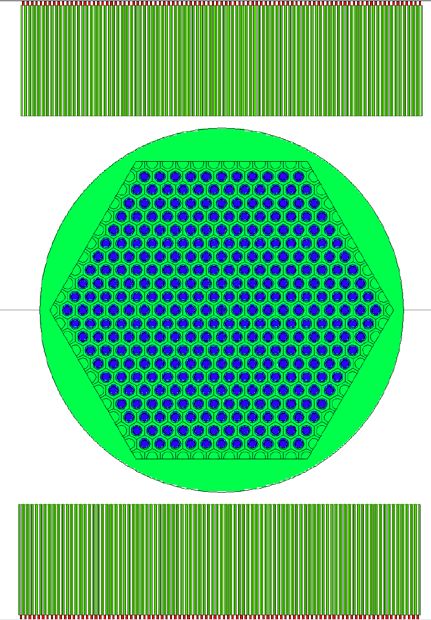
www.nature.com/scientificreports/

                                            Figure 5.  Image reconstructed using the inverse approach. Good contrast between the pin-present region and
                                            pin-absent region was achieved. No severe artifacts were observed on the reconstructed images.

                                            Figure 6.  Pin identifications based on the inverse approach. Identified pins are shown as red circles. For Cases 1
                                            to 5, we achieved 100% classification accuracy; for Case 6, we achieved 100% classification accuracy for the pins
                                            of medium and high activity level.

                                            Figure 7.  Activity distribution based on the inverse approach. The pin activity was estimated from each image
                                            by summing up the pixel values inside the present pins. The ground truth is shown as the red line.

                                            Figure 8.  Comparison of FISTA and PIDAL reconstruction to the ground truth. The two methods led to
                                            visually similar results, though the PIDAL reconstruction resulted in a sparser image, compared to FISTA.

                                            respectively. We applied both FISTA and PIDAL to perform reconstruction in Case 1 and compared them in
                                            Fig. 8. We assessed the image quality quantitatively using the mean-square-error (MSE) and structural similar-
                                            ity (SSIM)14. MSE is the mean-squared-difference between the reconstructed image and the ground truth, and
                                            SSIM measures the similarity between the reconstructed image and the ground truth. Lower MSE and higher
                                            SSIM mean better reconstruction. As shown in Table 1, the image reconstructed with FISTA resulted in a lower
                                            MSE and higher SSIM, compared to PIDAL, and PIDAL took approximately 20% longer to run than FISTA.
                                            Therefore, we used FISTA as the main image reconstruction algorithm.
                                                For comparison, we have also implemented the traditional FBP method to reconstruct the image, which is
                                            detailed in “Methods-image reconstruction methods" section. We then input these images to the neural network
                                            for pin identification, and estimated the pin activity levels. We compared the performance of the inverse (FISTA)
                                            and FBP approaches in terms of image quality, accuracy of pin identification and activity quantification. Fig. 9

          Scientific Reports |   (2021) 11:2442 |                https://doi.org/10.1038/s41598-021-82031-8                                                  4

Vol:.(1234567890)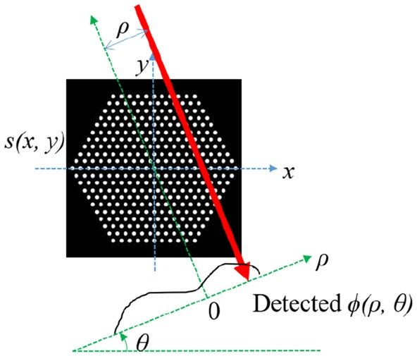
www.nature.com/scientificreports/

                                  Method                MSE                 SSIM               Computation time (s)
                                  PIDAL                 42.05               0.52               231.68
                                  FISTA                 41.45               0.59               183.57

                                  Table 1.  Comparison of MSE, SSIM, and computation time using FISTA and PIDAL. The computation time
                                  was measured on an Intel Core i9-7920X CPU.

                                  Figure 9.  Image reconstructed using FBP. Severe image blurring occurred at the center of Case1, Case 3 and
                                  Case 5.

                                              MSE                    SSIM                  Mis-classification rate
                                                                                           FBP                        INV
                                  Case        FBP         INV        FBP           INV     FP (%)         FN (%)      FP (%)     FN (%)
                                  1           96.62       41.45      0.16          0.59    0              1.51        0          0
                                  2           97.01       41.76      0.16          0.59    0.68           0           0          0
                                  3           95.32       40.69      0.16          0.56    0.34           0           0          0
                                   4          96.63       38.43      0.16          0.64    0              0           0          0
                                   5          88.70       37.38      0.17          0.60    0              3.40        0          0
                                   6          83.35       36.33      0.21          0.63    0              35.03       0          27.55

                                  Table 2.  Comparison of image quality and mis-classification rates for the six simulated cases reconstructed
                                  using traditional FBP and the inverse (INV) approach. FP: false positive (missing pins mis-classified as
                                  present) rate; FN: false negative (present pins mis-classified as missing) rate.

                                  Figure 10.  Pin identifications based on FBP. Identified pins are shown as red circles. Mis-classification of fuel
                                  pins appeared mostly at the center of Case 1, Case 3, and Case 5, where the hexagonal symmetry of the pin
                                  distribution was broken.

                                  shows the images reconstructed using FBP. Compared to Fig. 9, images in Fig. 5 demonstrated higher con-
                                  trast and fewer reconstruction artifacts. The blurring at the center was significantly removed using the inverse
                                  approach. We calculated the MSE and SSIM for both sets of images, shown in Table 2. We achieved significantly
                                  lower MSE and higher SSIM by using the inverse approach, which resulted in lower mis-classification rates of
                                  pin identification overall. The pin identification results based on FBP reconstruction are shown in Fig. 10. In
                                  Fig. 10a,c, and e, the blurring led to inaccurate pin localization around the center of FBP-reconstructed images,
                                  and the hexagonal structure was destroyed. In contrast, the hexagonal structure was accurately reproduced
                                  using the inverse problem approach, as shown in Fig. 6a–e. Hence, given the same sinogram data, the inverse
                                  approach is expected to better distinguish pins missing from the fuel assembly and result in lower false alarm
                                  rates, compared to FBP. MSE and SSIM are calculated based on unnormalized images. Therefore, in Case 6, we
                                  achieved the best MSE and SSIM because Case 6 exhibited the smallest average pixel intensity. Despite the good

Scientific Reports |   (2021) 11:2442 |                https://doi.org/10.1038/s41598-021-82031-8                                                      5

                                                                                                                                                Vol.:(0123456789)
www.nature.com/scientificreports/
Figure 11. Activity distribution based on FBP. The pin activity was estimated by multiplying a normalization
constant to the sum of all pixels inside the pin.The ground truth is shown as the red line.
Standard deviation
Mean NPS per pin (×107) Relative error (%) (%)
Case Truth FBP INV FBP INV FBP INV
1 1.51 1.57 1.57 3.91 3.74 6.16 4.36
2 1.70 1.72 1.74 1.39 2.21 7.57 3.44
3 1.70 1.71 1.73 − 0.68 2.02 8.54 5.09
4 1.70 1.72 1.73 1.12 1.46 7.71 3.33
5 1.70 1.65 1.66 − 2.91 − 2.25 15.75 6.85
Group 1 0.29 N.A. 0.39 N.A. 35.73 N.A. 14.22
6 Group 2 0.72 0.75 0.72 4.69 0.54 8.25 4.64
Group 3 1.44 1.42 1.43 − 1.25 − 0.59 10.68 3.70
Table 3. Comparison of activity estimations. The mean NPS per pin is the mean of the activity distribution;
relative error is the relative difference between the mean activity and ground truth; standard deviation refers to
the standard deviation of the pin activity distribution. For FBP in Group 1 of Case 6, no data is shown because
no present pin is identified.
image reconstruction, both FBP and inverse approaches led to relatively high mis-classification rates in Case 6
due to the fact that the low activity pins and high gradient in the pin activity are absent features in the training
set. However, we do not expect such a large variation of pin activities in an actual fuel a ssembly15 and, should
that be the case, a new training set can be used to improve the pin identification results.
We estimated the activity of each pin by summing the pixels on the reconstructed images and created a histo-
gram of pin activities for each case, shown in Figs. 7 and 11. It should be noted that for the FBP reconstruction,
there is no definite relationship between the pixel sum and the absolute activity. Appropriate normalization
constant needs to be applied to convert the pixel sum into activity, which is not always possible in an actual
inspection. In this case, we calculated the ratio between the mean of the pixel sum distribution and the true
activity for Cases 2–5. We then used the average of these ratios as the normalization constant and applied it to
all cases to convert the pixel sum to absolute activity. In contrast, normalization is not needed for the inverse
reconstruction because the response matrix has already been normalized per unit source particle. Compared
to Fig. 11, the pin activity distributions in Fig. 7 were narrower. We calculated the relative error compared to
the ground truth and the standard deviation of pin activity, as shown in Table 3. We obtained smaller standard
deviations by using the inverse approach in all cases. The relative error was negligible compared to the ground
truth, except for the low activity pins in Group 1 of Case 6.
Compared to UO2 fuel rod, the cobalt rod simulated in this work resulted in less attenuation because of
its lower density and atomic number. Nevertheless, this work describes a general approach for correcting the
gamma-ray attenuation and down-scattering in the energy window of interest and it can be easily adapted to
UO2 fuel assemblies by updating the atomic composition and gamma-ray source term in the simulation. In this
work, we assumed that the detector performance is the same in the simulation of the sinogram and response
matrix, which is not true for the real PGET device. The correction for varying detector performances across
the detectors, either at the hardware or software level, is crucial to obtain an accurate estimation of pin activity.
When identifying drifting detectors in post-processing, e.g., whose response is anomalously different compared
to neighbour detectors, a simple approach consists in neglecting their response. In a preliminary analysis on
simulated data, we replaced the response of an increasing number of detectors in the sinogram with null arrays.
We found that if the number of “neglected” detectors is below ten in the PGET setup, the reconstructed image
is negligibly affected by not including their response. Future work will be needed to study the robustness of the
software suite as a function of a systematic bias in the detector performance.
Conclusion
In this work, we have implemented a full set of software, which is able to reconstruct cross-sectional images of
mockup fuel assemblies acquired by a simulated PGET system, identify missing fuel pins, and estimate fuel pin
activities based on the reconstructed image. We have developed a linear forward model that accounts for the
scattering of gamma rays in the assembly to accurately characterize the response matrix of the PGET system.
Scientific Reports | (2021) 11:2442 | https://doi.org/10.1038/s41598-021-82031-8 6
Vol:.(1234567890)www.nature.com/scientificreports/
CdTe detector Helium gas
Tungsten collimator Cobalt pin
Aluminum cladding Water
Figure 12. The cross-sectional view of the MCNP model in Case 1. The hexagonal fuel assembly contains
331 60Co rods and is submerged in a water cylinder of 33 cm diameter. The fuel pin is simulated as a 60Co
cylinder of 7 mm diameter, coated with 1 mm thick aluminum cladding. Gamma rays emitted by the 60Co
rods are detected by two collimated CdTe detector arrays located on two sides of the fuel assembly, each
encompassing 91 detectors. The tungsten collimator between the detector array and fuel assembly is 10 cm
long and has an aperture of 1.5 mm. Each CdTe detector is closely attached to the collimator and is of size
0.175 × 0.35 × 0.35 cm3. The distance between two neighbouring detectors is 4 mm. The bottom array is shifted
to left by 2 mm, with respect to the top one3,4. The detector arrays rotate clockwise and scan the fuel bundle in
steps of 1◦, which generates a 182 × 360 sinogram.
The image reconstruction was formulated into a linear inverse problem by modeling the observation noise as
Gaussian, which was solved using FISTA. The reconstructed image was fed to a convolutional neural network
to automatically identify the present pins and determine their centroids. Compared to the FBP approach, the
inverse problem approach resulted in over 50% lower MSE and 200% higher SSIM, and consequently lower mis-
classification rates in pin identification in all cases. Based on the pin identification results, we estimated the pin
activity by summing up the pixel values around the centroid inside the pin radius on the image. Compared to
the FBP, the inverse approach resulted in smaller standard deviations of pin activity in all cases, with negligible
bias with respect to the ground truth. The proposed inverse approach to reconstruct a fuel pin cross section,
identify fuel pins and calculate their activity took approximately 8 minutes to run on an Intel Core i9-7920X CPU
without parallelization. We are currently improving the algorithm to allow automatic classification of different
activity groups in a real fuel assembly.
Methods
Monte Carlo simulation of the PGET based on MCNP. Figure 12 shows the cross-sectional view of
the MCNP model of Case 1. In Case 4 and 5, depleted uranium pins were used, where Co was replaced by 0.20%
enrichment UO 2 . We used the F4 tally as the detector response model in the MCNP simulation and the response
matrix calculation. The F4 tally estimates the average photon flux in the detector cell by summing the track
lengths of all particles in the 700-1500 keV energy window. The absolute activity measurement can be obtained
using the proposed method as long as the simulated quantity in the response matrix is consistent with the simu-
lated response to an unknown inspected fuel bundle. When applying the proposed technique to experimental
data, one would want to validate the simulated detector response with the measured one, to properly incorporate
specific detector’s properties, such as its energy resolution and time response, in the simulated model.
Image reconstruction methods. In this section, we describe in detail the two image reconstruction
methods implemented in this work: the FBP and linear inverse problem method. We applied both methods to
reconstruct images from the sinograms and compared their performance.
Filtered back‑projection. Figure 13 shows the tomography measurement of the fuel assembly at angle θ . The
FBP method relies on two approximations: first, we neglect the attenuation and scattering of gamma rays in the
system; second, for pins at different locations, we assume that the geometric efficiencies are the same. Under
these approximations, the sinogram φ(ρ, θ ) can be simplified as the integral of the source distribution s(x, y)
along the red line passing through the detector center, i.e.,
φ(ρ, θ ) = s(x, y)δ(x cos θ + y sin θ − ρ)dxdy. (1)
R2
Equation (1) is the standard forward model in X-ray tomography imaging. The classical inverse operation
from the sinogram to the source is the filtered back-projection, which is also a standard imaging algorithm in
X-ray imaging16 and will not be detailed here.
Scientific Reports | (2021) 11:2442 | https://doi.org/10.1038/s41598-021-82031-8 7
Vol.:(0123456789)www.nature.com/scientificreports/
Figure 13. The tomography measurement of the fuel assembly at an angle θ . The counts of detector (ρ, θ) can
be approximated by the integral of the source distribution s(x, y) along the red line that passes through the
detector center.
Inverse problem approach. The inverse reconstruction approach is based on the conversion of the image recon-
struction problem into a linear inverse problem. Let the vectorized image of the fuel assembly be s , which con-
tains N unknown pixel values, and the vectorized simulated sinogram of size M = 65, 520 (182 × 360) be φ . The
inverse approach relies on the assumption that φ is a linear function of s ,
φ = As + n, (2)
where A is the system response matrix of size M × N , and n models random observation noise, assumed to be
isotropic Gaussian distributed. Physically, the i-th column of the response matrix A is the vectorized sinogram
corresponding to a pin distribution with unit activity in pixel i but zero elsewhere. Accurate determination of
the system response matrix is crucial to obtain a high-quality image and avoid systematic bias in pin identifica-
tion and activity estimation. The analytical derivation of the response matrix is discussed in the next section.
Given the simulated sinogram and system response matrix A , we can reconstruct the image by solving the
following equation:
N
1 2 1 T
ŝ = argmin �φ − As�2 + �s�1 = argmin (φ − As) (φ − As) + |si | (3)
si ≥0,∀i 2 si ≥0,∀i 2
i=1
where the first term is the data-fidelity term assuming Gaussian noise, and the second term is a regularization
term acknowledging that the fuel pin is sparsely distributed. The regularization parameter is chosen based
on the noise level. To solve Eq. (3), we have implemented the fast iterative shrinkage-thresholding algorithm
(FISTA)12.
As an alternative, we can model the observation noise by Poisson noise and the data-fidelity term is changed
accordingly13,17 as follows
�M
ŝ = argmin ([As]j − φ j log[As]j ) + �s�1 . (4)
si ≥0,∀i j=1
To solve Eq. (4), we used the PIDAL algorithmic structure described i n13.
Computation of the response matrix. The calculation of the system response matrix A involves the calculation
of detector response to each pixel, with each response being one column in the matrix. For inner pixels, the
contribution from scattered photons is non-negligible due to the high attenuation. To account for this, we have
implemented an algorithm that combines stochastic photon transport with deterministic collimator-detector
modeling to accurately calculate the system response matrix.
For real fuel assemblies, no prior information of pin distribution and pin radius will be given. It is therefore
necessary to first estimate these quantities before running the Monte Carlo simulation. As discussed in the
“Results-Inverse approach” section, this is done by performing a rough image reconstruction using our previ-
ously developed model, where uniform attenuation map is used and no scattering effect is c onsidered11. Based
on the reconstructed image, one could determine the pin locations and pin radius, and create a material map,
where the material is assumed to be cobalt inside the pin, and water outside.
Next, we simulate the travel of photons inside the fuel assembly using Monte Carlo. Two sets of grids are
generated. The fine grid has a pixel size of 0.5 × 0.5 mm 2 , while the coarse grid has a pixel size of 2 × 2 mm 2 .
We first discretize the region of interest on the fine grid and calculate the response to the pixels whose center
points are inside the pin. Then we calculate the response to a pixel on the coarse grid by summing the responses
to the corresponding 4 × 4 pixels on the fine grid. Based on the pin identification result in the previous step, the
potential pin-present region are pixelated into 5329 coarse pixels. We iterate over all these pixels and form the
response matrix. In this way, we are able to reduce the pixelization error introduced during the discretization of
the pins, without increasing the final response matrix size.
Scientific Reports | (2021) 11:2442 | https://doi.org/10.1038/s41598-021-82031-8 8
Vol:.(1234567890)www.nature.com/scientificreports/
Detection unit
Medium
Photon
Photon travel path
Forced detection path
Figure 14. Illustration of the CFD technique. A photon shown as the gray disk is created on the left and travels
in the medium along the solid arrow. The disk radius represents the photon energy. Upon it creation and each
interaction with the medium, the photon is forced to be scattered along the dash arrow and to be detected by the
detector with a certain probability.
The response to each fine pixel whose center point is inside the pin is calculated in the following way. A pho-
ton (r0 , �0 , E0 , W0 ) is created, with the initial position r0 uniformly sampled inside the pixel, the initial moving
direction 0 uniformly sampled in 4π space, the initial energy E0 sampled from the source energy spectrum, and
the initial weight W0 assigned to 1. We track the photon inside the PGET using the delta-tracking a lgorithm18
and determine the position where the photon interacts with medium. We force the interaction to be Compton
scattering by multiplying its weight with the probability that the interaction is Compton scattering,
µsc (ri−1 , Ei−1 )
Wi = Wi−1 (5)
µ(ri−1 , Ei−1 )
where µsc (ri−1 , Ei−1 ) and µ(ri−1 , Ei−1 ) are the Compton scattering attenuation coefficient and total attenuation
coefficient at the i-th interaction site, respectively. A scattering angle is sampled19, and the photon energy Ei and
moving direction i are updated accordingly. This process is repeated until the photon escapes the fuel assembly
or the photon energy is below the detection threshold. A copy of the photon is saved at its creation site and each
interaction site to a sub-projection map.
Once the sub-projection map is obtained, we apply the convolutional forced detection (CFD) technique
to calculate the detector response. CFD is a widely-used variance reduction technique for X-ray downscatter
simulation in single photon emission computed tomography (SPECT), which has been shown to be 50–100 times
faster than conventional forced detection t echnique20 and several thousand times faster than full-3D Monte
Carlo simulation21. Figure 14 illustrates its principle. In CFD, the photon is forced to travel perpendicularly to
the detector plane upon its creation or interaction with medium to effectively simulate all the possible spatial
distributions of particle interactions and consequent detection events. For an unscattered photon, the contribu-
tion to the F4 tally in the detector cell is given by
�� Tl
W× × e− µ(r,E)ds × (6)
4π V
and for a scattered photon, the contribution is
σ (θ)�� Tl
W× π
′ ′ ′
× e− µ(r,E(θ ))ds × . (7)
2π 0 σ (θ ) sin(θ )dθ V
In Eqs. (6) and (7), W is the photon weight,
is the solid angle subtended by the detector in steradian,
σ (θ) is the differential cross-section for Compton scattering, µ(r, E) is the total attenuation coefficient along
the CFD path, and the last term stands for the contribution to F4 tally, i.e., average track length in detector cell
normalized by detector volume.
Due to the non-ideal collimation, a photon will contribute counts not only to the detector in the same col-
umn, but also to the neighbouring ones. This phenomenon is characterized by the depth-dependent point spread
function (PSF) of the collimator, i.e., the photon count distribution on the detection plane when a point source
is imaged. PSF depends on the vertical distance z between the photon and the detector array22:
√
−4 ln 2 × x 2
2 ln(2) b 2
PSFz (x) = √ exp 2
, FWHM(z) = b + z, leff = l − (8)
πFWHM(z) FWHM(z) leff µ
where b is the collimator aperture, l is the collimator length, µ is the total attenuation coefficient in the collimator,
and FWHM is the width of the collimator PSF.
To calculate the response to a pin at an angle θ , the photons saved in the sub-projection map are first rotated by
an angle −θ . We then sum the weights of the photons in the same pixel on the sub-projection map and calculate
their contribution to the detector response based on Eqs. (6) or (7), which creates a projection map. We then
Scientific Reports | (2021) 11:2442 | https://doi.org/10.1038/s41598-021-82031-8 9
Vol.:(0123456789)www.nature.com/scientificreports/
convolve each row in the projection map with the PSF function and sum all rows up to get the response at this
angle. Next, we increment the angle θ and calculate the response at the next angle. In this way, photon tracking
in the fuel assembly is done only once, which saves computation time.
We simulated the travel of 6400 photons to create the sub-projection map for one pixel. It took approximately
4 mins to calculate the response matrix containing 5329 pixels using CFD on an Intel Core i9-7920X CPU.
Pin localization. Images reconstructed using both approaches are input to a convolution neural network,
referred to as U-net23, to perform pin identification. The experimental data provided by IAEA within the frame-
work of a technology open challenge7 were used for the training of the U-net. The training data consisted of the
FBP images reconstructed from the measured sinograms of mock-up assemblies of 12 different geometries with
a variable number of 60Co pins, and examples of the reconstructed images of these assemblies can be found in7.
The U-net was trained to minimize a binary crossentropy loss between the predicted pin masks and ground
truth. For each image, we provided four randomly rotated ones as input to the network, for data augmentation.
Data augmentation allowed us to generate new training instances from existing ones, artificially boosting the
size of the training set. The network was trained for 10,000 epochs, i.e., complete iteration over the whole dataset,
using a learning rate of 10−5 and an Adam optimizer24. We found that 10−5 is the learning rate for which the slope
of the crossentropy loss is maximized, allowing to reach the minimum. The training was early stopped when the
loss reached its minimum value. The trained U-net can extract visible structures from the input image and out-
put a mask based on the extracted features. Bright regions on the mask with areas above a certain threshold are
identified as present pins, and their centroids are calculated as the coordinates of the center of each pin.
Received: 9 September 2020; Accepted: 7 January 2021
References
1. United Nations Office for Disarmament Affairs. Treaty on the non-proliferation of nuclear weapons (1970). http://disarmamen
t.un.org/treaties/t/npt/text.
2. ElBaradei, M. Addressing verification challenges. In Proceedings of an International Safeguards Symposium, 21 (Vienna, 2006).
3. Honkamaa, T. et al. A prototype for passive gamma emission tomography (In Proc. Symp. Int, Safeguards, 2014).
4. White, T. et al. Application of passive gamma emission tomography (pget) for the verification of spent nuclear fuel. In INMM 59th
Annual Meeting, Baltimore, Maryland, USA (2018).
5. Mayorov, M. et al. Gamma emission tomography for the inspection of spent nuclear fuel. In 2017 IEEE Nuclear Science Symposium
and Medical Imaging Conference (NSS/MIC), 1–2 (2017).
6. SCK CEN. Use of the fork detector in safeguards inspections (2007). https://inis.iaea.org/collection/NCLCollectionStore/_Publi
c/40/100/40100153.pdf.
7. IAEA. Iaea tomography reconstruction and analysis challenge. https://ideas.unite.un.org/iaea-tomography/Page/Home (2018).
Accessed 12 Jun 2020.
8. Backholm, R. et al. Simultaneous reconstruction of emission and attenuation in passive gamma emission tomography of spent
nuclear fuel. Inverse Probl. Imaging 14, 317. https://doi.org/10.3934/ipi.2020014 (2020).
9. Goorley, J. T. et al. Initial mcnp6 release overview-mcnp6 version 1.0. Tech. Rep., Los Alamos National Lab. (LANL), Los Alamos
(2013).
10. Di Fulvio, A. et al. Neutron rodeo phase ii final report. Tech. Rep., Argonne National Lab. (ANL), Argonne, IL (2019).
11. Fang, M., Latta, D. D., Altmann, Y., Salvatori, M. & Fulvio, A. D. Comparison of Image Reconstruction Methods for Simulated
Passive Gamma Emission Tomography. In INMM 61st Annual Meeting (Baltimore, 2020).
12. Beck, A. & Teboulle, M. A fast iterative shrinkage-thresholding algorithm for linear inverse problems. SIAM J. Imaging Sci. 2,
183–202 (2009).
13. Figueiredo, M. A. T. & Bioucas-Dias, J. Restoration of Poissonian images using alternating direction optimization. IEEE Trans.
Image Process. 19, 3133–3145. https://doi.org/10.1109/TIP.2010.2053941 (2010).
14. Wang, Z., Bovik, A. C., Sheikh, H. R. & Simoncelli, E. P. Image quality assessment: From error visibility to structural similarity.
IEEE Trans. Image Process. 13, 600–612 (2004).
15. Jardine, L. Radiochemical assays of irradiated vver-440 fuel for use in spent fuel burnup credit activities (Tech. Rep, Lawrence Liv-
ermore National Lab, 2005).
16. Prince, J. L. & Links, J. M. Medical Imaging Signals and Systems (Pearson Prentice Hall, Upper Saddle River, 2006).
17. Lefkimmiatis, S. & Unser, M. Poisson image reconstruction with Hessian Schatten-norm regularization. IEEE Trans. Image Process.
22, 4314–4327 (2013).
18. Woodcock, E., Murphy, T., Hemmings, P. & Longworth, S. Techniques used in the gem code for monte carlo neutronics calcula-
tions in reactors and other systems of complex geometry. In Proc. Conf. Applications of Computing Methods to Reactor Problems,
vol. 557 (1965).
19. Kahn, H. Applications of Monte Carlo (RAND Corp., Santa Monica, 1954).
20. Hutton, B. F., Buvat, I. & Beekman, F. J. Review and current status of spect scatter correction. Phys. Med. Biol. 56, R85 (2011).
21. Beekman, F. J., de Jong, H. W. & van Geloven, S. Efficient monte carlo based reconstruction for general quantitative spect. In 2001
IEEE Nuclear Science Symposium Conference Record (Cat. No. 01CH37310), vol. 4, 1864–1868 (IEEE, 2001).
22. de Jong, H. W., Slijpen, E. T. & Beekman, F. J. Acceleration of Monte Carlo spect simulation using convolution-based forced detec-
tion. IEEE Trans. Nuclear Sci. 48, 58–64 (2001).
23. Ronneberger, O., Fischer, P. & Brox, T. U-net: Convolutional networks for biomedical image segmentation. In International Confer‑
ence on Medical image computing and computer-assisted intervention, 234–241 (Springer, 2015).
24. Kingma, D. P. & Ba, J. Adam: A method for stochastic optimization. arXiv:1412.6980 (2014).
Acknowledgements
This work was funded in part by the Nuclear Regulatory Commission Faculty Development Grant Number
31310019M0011 and the Consortium for Verification Technology under Department of Energy National Nuclear
Security Administration Award Number DE-NA0002534. This work was also supported by the Royal Academy
of Engineering under the Research Fellowship scheme RF201617/16/31.
Scientific Reports | (2021) 11:2442 | https://doi.org/10.1038/s41598-021-82031-8 10
Vol:.(1234567890)www.nature.com/scientificreports/
Author contributions
M.F. developed the forward model and analyzed the data, Y.A. implemented the FISTA and PIDAL algorithms,
D.D.L. and M.S. developed and trained the neural network, A.D.F. implemented the FBP and the MC model,
conceived and oversaw the project. M.F., Y.A., A.D.F., and M.S. wrote the manuscript. All authors reviewed the
manuscript.
Competing interests
The authors declare no competing interests.
Additional information
Correspondence and requests for materials should be addressed to M.F.
Reprints and permissions information is available at www.nature.com/reprints.
Publisher’s note Springer Nature remains neutral with regard to jurisdictional claims in published maps and
institutional affiliations.
Open Access This article is licensed under a Creative Commons Attribution 4.0 International
License, which permits use, sharing, adaptation, distribution and reproduction in any medium or
format, as long as you give appropriate credit to the original author(s) and the source, provide a link to the
Creative Commons licence, and indicate if changes were made. The images or other third party material in this
article are included in the article’s Creative Commons licence, unless indicated otherwise in a credit line to the
material. If material is not included in the article’s Creative Commons licence and your intended use is not
permitted by statutory regulation or exceeds the permitted use, you will need to obtain permission directly from
the copyright holder. To view a copy of this licence, visit http://creativecommons.org/licenses/by/4.0/.
© The Author(s) 2021
Scientific Reports | (2021) 11:2442 | https://doi.org/10.1038/s41598-021-82031-8 11
Vol.:(0123456789)You can also read