Quantum-inspired machine learning on high-energy physics data
←
→
Page content transcription
If your browser does not render page correctly, please read the page content below
www.nature.com/npjqi

                  ARTICLE                  OPEN

                  Quantum-inspired machine learning on high-energy physics
                  data
                  Timo Felser 1,2,3,4 ✉, Marco Trenti1,2, Lorenzo Sestini                  3
                                                                                               , Alessio Gianelle    3
                                                                                                                         , Davide Zuliani2,3, Donatella Lucchesi            2,3
                                                                                                                                                                                  and
                  Simone Montangero 2,3,5

                      Tensor Networks, a numerical tool originally designed for simulating quantum many-body systems, have recently been applied to
                      solve Machine Learning problems. Exploiting a tree tensor network, we apply a quantum-inspired machine learning technique to a
                      very important and challenging big data problem in high-energy physics: the analysis and classification of data produced by the
                      Large Hadron Collider at CERN. In particular, we present how to effectively classify so-called b-jets, jets originating from b-quarks
                      from proton–proton collisions in the LHCb experiment, and how to interpret the classification results. We exploit the Tensor
                      Network approach to select important features and adapt the network geometry based on information acquired in the learning
                      process. Finally, we show how to adapt the tree tensor network to achieve optimal precision or fast response in time without the
                      need of repeating the learning process. These results pave the way to the implementation of high-frequency real-time applications,
                      a key ingredient needed among others for current and future LHCb event classification able to trigger events at the tens of
                      MHz scale.
1234567890():,;

                      npj Quantum Information (2021)7:111 ; https://doi.org/10.1038/s41534-021-00443-w

                  INTRODUCTION                                                                               ML16,30. Hereafter, we demonstrate the effectiveness of the
                  Artificial Neural Networks (NN) are a well-established tool for                             approach and, more importantly, that it allows introducing
                  applications in Machine Learning and they are of increasing                                algorithms to simplify and explain the learning process, unveiling
                  interest in both research and industry1–6. Inspired by biological                          a pathway to an explainable Artificial Intelligence. As a potential
                  NN, they are able to recognise patterns while processing a huge                            application of this approach, we present a TN supervised learning
                  amount of data. In a nutshell, a NNs describes a functional                                of identifying the charge of b-quarks (i.e. b or b) produced in high-
                  mapping containing many variational parameters, which are                                  energy proton–proton collisions at the Large Hadron Collider
                  optimised during the training procedure. Recently, deep connec-                            (LHC) accelerator at CERN.
                  tions between Machine Learning and quantum physics have been                                  In what follows, we first describe the quantum-inspired Tree
                  identified and continue to be uncovered7. On one hand, NNs have                             Tensor Network (TTN) and introduce different quantities that can
                  been applied to describe the behaviour of complex quantum                                  be extracted from the TTN classifier which are not easily accessible
                  many-body systems8–10 while, on the other hand, quantum-                                   for the biological-inspired Deep NN (DNN), such as correlation
                  inspired technologies and algorithms are taken into account to                             functions and entanglement entropy which can be used to explain
                  solve Machine Learning tasks11–13.                                                         the learning process and subsequent classifications, paving the
                     One particular numerical method originated from quantum                                 way to an efficient and transparent ML tool. In this regard, we
                  physics which has been increasingly compared to NNs are Tensor                             introduce the Quantum-Information Post-learning feature Selec-
                  Networks (TNs)14–16. TNs have been developed to investigate                                tion (QuIPS), a protocol that reduces the complexity of the ML
                  quantum many-body systems on classical computers by efficiently                             model based on the information the single features provide for
                  representing the exponentially large quantum wavefunction jψi in                           the classification problem. We then briefly describe the LHCb
                  a compact form and they have proven to be an essential tool for a                          experiment and its simulation framework, the main observables
                  broad range of applications17–26. The accuracy of the TN                                   related to b-jets physics, and the relevant quantities for this
                  approximation can be controlled with the so-called bond-                                   analysis together with the underlying LHCb data33,34. We further
                  dimension χ, an auxiliary dimension for the indices of the                                 compare the performance obtained by the DNN and the TTN,
                  connected local tensors. Recently, it has been shown that TN                               before presenting the analytical insights into the TTN which,
                  methods can also be applied to solve Machine Learning (ML) tasks                           among others, can be exploited to improve future data analysis of
                  very effectively13,16,27–31. Indeed, even though NNs have been                             high-energy problems for a deeper physical understanding of the
                  highly developed in recent decades by industry and research, the                           LHCb data. Moreover, we introduce the Quantum-Information
                  first approaches of ML with TN yield already comparable results                             Adaptive Network Optimisation (QIANO), which adapts the TN
                  when applied to standard datasets13,27,32. Due to their original                           representation by reducing the number of free parameters based
                  development focusing on quantum systems, TNs allow to easily                               on the captured information within the TN while aiming to
                  compute quantities such as quantum correlations or entangle-                               maintain the highest accuracy possible. Therewith, we can
                  ment entropy and thereby they grant access to insights on the                              optimise the trained TN classifier for a targeted prediction speed
                  learned data from a distinct point of view for the application in                          without the necessity to relearn a new model from scratch.

                  1
                   Tensor Solutions, Institute for Complex Quantum Systems, University of Ulm, Ulm, Germany. 2Dipartimento di Fisica e Astronomia G. Galilei, Università di Padova, Padova, Italy.
                  3
                   INFN, Sezione di Padova, Padova, Italy. 4Theoretische Physik, Universität des Saarlandes, Saarbrücken, Germany. 5Padua Quantum Technologies Research Center, Università degli
                  Studi di Padova, Padova, Italy. ✉email: timo.felser@tensor-solutions.com

                  Published in partnership with The University of New South Wales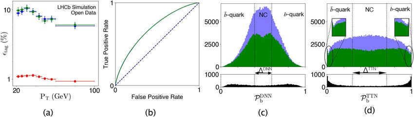
T. Felser et al.
                  2

                      Fig. 1 Data flow of the Machine Learning analysis for the b-jet classification of the LHCb experiment at CERN. After proton–proton
                      collisions, b- and b-quarks are created, which subsequently fragment into particle jets (left). The different particles within the jets are tracked
                      by the LHCb detector. Selected features of the detected particle data are used as input for the Machine Learning analysis by NNs and TNs in
                      order to determine the charge of the initial quark (right).
1234567890():,;

                         TNs are not only a well-established way to represent a quantum            weighted probabilities
                      wavefunction jψi, but more general an efficient representation of
                      information as such. In the mathematical context, a TN                             jhΦðxÞjψl ij2
                                                                                                   Pl ¼ P                2
                                                                                                                                                                      (4)
                      approximates a high-order tensor by a set of low-order tensors                      l jhΦðxÞjψl ij
                      that are contracted in a particular underlying geometry and have
                                                                                                   for each class. We point out, that we can encode the input data in
                      common roots with other decompositions, such as the Singular
                                                                                                   different non-linear feature maps as well (see Supplementary
                      Value Decomposition (SVD) or Tucker decomposition35. Among
                                                                                                   Notes).
                      others, some of the most successful TN representations are the
                                                                                                      One of the major benefits of TNs in quantum mechanics is the
                      Matrix Product State—or Tensor Trains18,27,36,37, the TTN—or
                                                                                                   accessibility of information within the network. They allow to
                      Hierarchical Tucker decomposition30,38,39, and the Projected
                                                                                                   efficiently measure information quantities such as entanglement
                      Entangled Pair States40,41.
                                                                                                   entropy and correlations. Based on these quantum-inspired
                         For a supervised learning problem, a TN can be used as the
                                                                                                   measurements, we here introduce the QuIPS protocol for the TN
                      weight tensorW13,27,30, a high-order tensor which acts as classifier
                                                                                                   application in ML, which exploits the information encoded and
                      for the input data {x}: Each sample x is encoded by a feature map            accessible in the TN in order to rank the input features according
                      Φ(x) and subsequently classified by the weight tensor W. The final             to their importance for the classification.
                      confidence of the classifier for a certain class labelled by l is given           In information theory, entropy as such is a measure of the
                      by the probability                                                           information content inherent in the possible outcomes of
                      P l ðxÞ ¼ W l  ΦðxÞ :                                                (1)    variables, such as e.g. a classification42–44. In TNs such information
                                                                                                   content can be assessed by means of the entanglement entropy S
                        In the following, we use a TTN Ψ to represent W (see Fig. 1,               which describes the shared information between TN bipartitions.
                      bottom right) which can be described as a contraction of its N               The entanglement S is measured via the Schmidt decomposition,

                      hierarchically connected local tensors T{χ}                                  that is, decomposing jψi into two bipartitions ψAα and ψBα 44
                                                                                                   such that
                            X      ½1
                                                Y
                                                N
                      Ψ ¼        T l;χ 1 ;χ 2         T χ½ηn ;χ 2n ;χ 2n þ 1               (2)          X
                                                                                                         χ
                             χ                  η¼2                                                Ψ ¼        λα ΨAα  ΨBα ;                                        (5)
                                                                                                          α
                      where n ∈ [1, N]. Therefore, we can interpret the TTN classifier Ψ as
                                                                                                   where λα are the Schmidt-coefficients (non-zero, normalised
                      well as a set of quantum many-body wavefunctions jψl i—one for
                                                                                                   singular values of the decomposition). The entanglement entropy
                      each of the class labels l (see Supplementary Methods). For the                                           P
                      classification, we represent each sample x by a product state Φ(x).           is then defined as S ¼  α λ2α ln λ2α . Consequently, the minimal
                      Therefore, we map each feature xi ∈ x into a quantum spin by                 entropy S = 0 is obtained only if we have one single non-zero
                      choosing the feature map Φ(x) as a Kronecker product of N + 1                singular value λ1 = 1. In this case, we can completely separate the
                      local feature maps                                                           two bipartitions as they share no information. On the contrary,
                                      0          0                                           higher S means that information is shared among the bipartitions.
                                         πx         πx i                                              In the ML context, the entropy can be interpreted as follows: If
                       Φ½i ðx i Þ ¼ cos     ; sin                                     (3)         the features in one bipartition provide no valuable information for
                                          2          2
                                                                                                   the classification task, the entropy is zero. On the contrary, S
                      where x 0  x i =x i;max 2 ½0; 1 is the re-scaled value with respect to     increases the more information between the two bipartitions are
                      the maximum xi,max within all samples of the training set.                   exploited. This analysis can be used to optimise the learning
                        Accordingly, we classify a sample x by computing the overlap               procedure: whenever S = 0, the feature can be discarded with no
                      ⟨Φ(x)∣ψl⟩ for all labels l with the product state Φ(x) resulting in the      loss of information for the classification. Thereby, a second model

                      npj Quantum Information (2021) 111                                                  Published in partnership with The University of New South Wales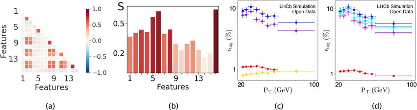
T. Felser et al.
                                                                                                                                                          3
with fewer features and fewer tensors can be introduced. This               account the efficiency ϵeff (the fraction of jets for which the
second, more efficient model results in the same predictions in              classifier takes a decision) and the prediction accuracy a (the
less time. On the contrary, a high bipartition entropy highlights           fraction of correctly classified jets among them) as follows:
which feature—or combination of features—are important for the
correct predictions.                                                        ϵtag ¼ ϵeff  ð2a  1Þ2 :                                               (7)
   The second set of measurements we take into account are the              To date, the muon tagging method gives the best performance on
correlation functions                                                       the b- vs. b-jet discrimination using the dataset collected in the
           hψl jσzi σzj jψl i                                               LHC Run I58: here, the muon with the highest momentum in the
C li;j ¼                                                              (6)   jet is selected, and its electric charge is used to decide on the b-
             hψl jψl i
                                                                            quark charge.
for each pair of features (located at site i and j) and for each class l.      For the ML application, we now formulate the identification of
The correlations offer an insight into the possible relation among          the b-quark charge in terms of a supervised learning problem. As
the information that the two features provide. In case of maximum           described above, we implemented a TTN as a classifier and
correlation or anti-correlation among them for all classes l, the           applied it to the LHCb problem analysing its performance.
information of one of the features can be obtained by the other             Alongside, a DNN analysis is performed to the best of our
one (and vice versa), thus one can be neglected. In case of no              capabilities, and both algorithms are compared with the muon
correlation among them, the two features may provide funda-                 tagging approach. Both the TTN and the DNN, use as input for the
mentally different information for the classification. The correla-          supervised learning 16 features of the jet substructure from the
tion analysis allows pinpointing if two features give independent           official simulation data released by the LHCb collaboration33,34.
information. However, the correlation itself—in contrast to the             The 16 features are determined as follows: the muon with the
entropy—does not tell if this information is important for the              highest pT among all other detected muons in the jet is selected
classification.                                                              and the same is done for the highest pT kaon, pion, electron, and
   In conclusion, based on the previous insights, namely: (i) a low         proton, resulting in 5 different selected particles. For each particle,
entropy of a feature bipartition signals that one of the two                three observables are considered: (i) The momentum relative to
bipartitions can be discarded, providing negligible loss of                 the jet axis (prel
                                                                                             T ), (ii) the particle charge (q), and (iii) the distance
information and (ii) if two features are completely (anti-)correlated       between the particle and the jet axis (ΔR), for a total of 5 × 3
we can neglect at least one of them, the QuIPS enables to filter out         observables. If a particle type is not found in a jet, the related
the most valuable features for the classification.                           features are set to 0. The 16th feature is the total jet charge Q,
   Nowadays, in particle physics, ML is widely used for the                 defined as the weighted average of the particles charges qi inside
classification of jets, i.e. streams of particles produced by the            the jet, using the particles prel T as weights:
fragmentation of quarks and gluons. The jet substructure can be                    P rel
                                                                                       ðp Þ q
exploited to solve such classification problems45. ML techniques              Q ¼ Pi T rel i i :                                                     (8)
have been proposed to identify boosted, hadronically decaying                          i ðpT Þi
top quarks46, or to identify the jet charge47. The ATLAS and CMS
collaborations developed ML algorithms in order to identify jets
generated by the fragmentation of b-quarks48–50: a comprehen-               RESULTS
sive review on ML techniques at the LHC can be found in51.                  Analysis framework
   The LHCb experiment in particular is, among others, dedicated
                                                                            In the following, we present the jet classification performance for
to the study of the physics of b- and c-quarks produced in
                                                                            the TTN and the DNN applied to the LHCb dataset, also comparing
proton–proton collisions. Here, ML methods have been introduced
                                                                            both ML techniques with the muon tagging approach. For the
recently for the discrimination between b- and c-jets by using
                                                                            DNN we use an optimised network with three hidden layers of 96
Boosted Decision Tree classifiers52. However, a crucial topic for the
                                                                            nodes (see Supplementary Methods for details). Hereafter, we aim
LHCb experiment, which is yet unexploited by ML, is the
                                                                            to compare the best possible performance of both approaches
identification of the charge of a b-quark, i.e. discriminating
                                                                            therefore, we optimised the hyperparameters of both methods in
between a b or b. Such identification can be used in many
                                                                            order to obtain the best possible results from each of them, TTN
physics measurements, and it is the core of the determination of
                                                                            and DNN. Therefore, we split the dataset of about 700k events
the charge asymmetry in b-pairs production, a quantity sensitive
                                                                            (samples) into two sub-sets: 60% of the samples are used in the
to physics beyond the Standard Model53. Whenever produced in a
                                                                            training process while the remaining 40% are used as test set to
scattering event, b-quarks have a short lifetime as free particles;
                                                                            evaluate and compare the different methods. For each event
indeed, they manifest themselves as bound states (hadrons) or as
                                                                            prediction after the training procedure, both ML models output
narrow cones of particles produced by the hadronization (jets). In
                                                                            the probability P b to classify the event as a jet generated by a b-
the case of the LHCb experiment, the b-jets are detected by the
                                                                            or a b-quark. A threshold Δ around P b ¼ 0:5 is then defined in
apparatus located in the forward region of proton–proton
                                                                            which we classify the quark as unknown in order to optimise the
collisions (see Fig. 1, left)54. The LHCb detector includes a particle
                                                                            overall tagging power ϵtag.
identification system that distinguishes different types of charged
particles within the jet, and a high-precision tracking system able
to measure the momentum of each particles55. Still, the separation          Jet classification performance
between b- and b-jets is a highly difficult task because the b-quark         We obtain similar performances in terms of the raw prediction
fragmentation produce dozens of particles via non-perturbative              accuracy applying both ML approaches after the training
Quantum Chromodynamics processes, resulting in non-trivial                  procedure on the test data: the TTN takes a decision on the
correlations between the jet particles and the original quark.              charge of the quark in ϵeff
                                                                                                    TTN
                                                                                                        ¼ 54:5% of the cases with an overall
   The algorithms used to identify the charge of the b-quarks               accuracy of aTTN = 70.56%, while the DNN decides in ϵeff  DNN
                                                                                                                                           ¼
based on information on the jets are called tagging methods. The            55:3% of the samples with a    DNN
                                                                                                               = 70.49%. We checked both
tagging algorithm performance is typically quantified with the               approaches for biases in physical quantities to ensure that both
tagging power ϵtag, representing the effective fraction of jets that        methods are able to properly capture the physical process behind
contribute to the statistical uncertainty in an asymmetry                   the problem and thus that they can be used as valid tagging
measurement56,57. In particular, the tagging power ϵtag takes into          methods for LHCb events (see Supplementary Methods).

Published in partnership with The University of New South Wales                                              npj Quantum Information (2021) 111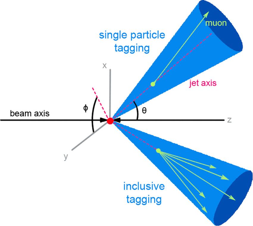
T. Felser et al.
4
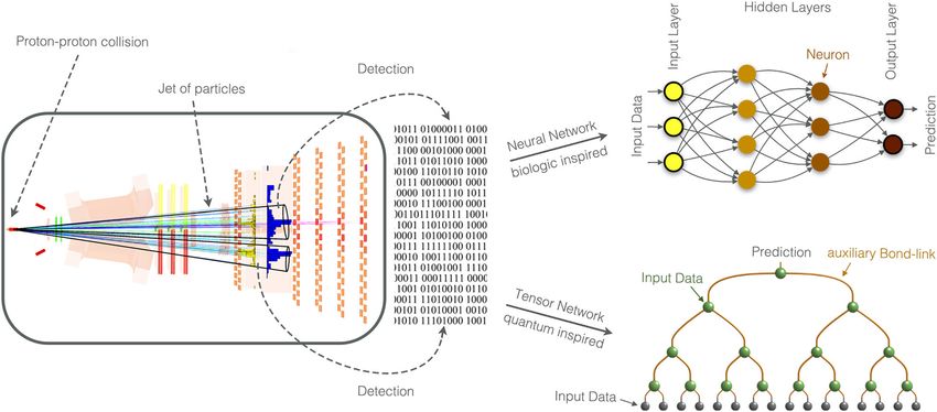
Fig. 2 Comparison of the DNN and TNN analysis. a Tagging power for the DNN (green), TTN (blue) and the muon tagging (red), (b) ROC
curves for the DNN (green) and the TTN (blue, but completely covered by DNN), compared with the line of no-discrimination (dotted navy-blue
line), (c) probability distribution for the DNN and (d) for the TTN. In the two distributions (c, d), the correctly classified events (green) are
shown in the total distribution (light blue). Below, in black all samples where a muon was detected in the jet.
Fig. 3 Exploiting the information provided by the learned TTN classifier. a Correlations between the 16 input features (blue for anti-
correlated, white for uncorrelated, red for correlated). The numbers indicate q, prelT , ΔR of the muon (1–3), kaon (4–6), pion (7–9), electron
(10–12), proton (13–15) and the jet charge Q (16). b Entropy of each feature as the measure for the information provided for the classification.
c Tagging power for learning on all features (blue), the best eight proposed by QuIPS exploiting insights from (a, b) (magenta), the worst eight
(yellow) and the muon tagging (red). d Tagging power for decreasing bond-dimension truncated after training: The complete model (blue
shades for χ = 100, χ = 50, χ = 5), for using the QuIPS best 8 features only (violet shades for χ = 16, χ = 5), and the muon tagging (red).
In Fig. 2a we present the tagging power of the different guessing classifier: the two ROC curves for TTN and DNN are
approaches as a function of the jet transverse momentum pT. perfectly coincident, and the Area Under the Curve (AUC) for the
Evidently, both ML methods perform significantly better than the two classifiers is the almost same (AUCTTN = 0.689 and AUCDNN =
muon tagging approach for the complete range of jet transverse 0.690). The graph illustrates the similarity in the outputs between
momentum pT, while the TTN and DNN display comparable TTN and DNN despite the different confidence distributions. This is
performances within the statistical uncertainties. further confirmed by a Pearson correlation factor of r = 0.97
In Fig. 2c, d we present the histograms of the confidences for between the outputs of the two classifiers.
predicting a b-flavoured jet for all samples in the test dataset for In conclusion, the two different approaches result in similar
the DNN and the TTN respectively. Interestingly, even though both outcomes in terms of prediction performances. However, the
approaches give similar performances in terms of overall precision underlying information used by the two discriminators is
and tagging power, the prediction confidences are fundamentally inherently different. For instance, the DNN predicts more
different. For the DNN, we see a Gaussian-like distribution with, in conservatively, in the sense that the confidences for each
general, not very high confidence for each prediction. Thus, we prediction tend to be lower compared with the TTN. Additionally,
obtain less correct predictions with high confidences, but at the the DNN does not exploit the presence of the muon as strongly as
same time, fewer wrong predictions with high confidences the TTN, even though the muon is a good predictor for the
compared to the TTN predictions. On the other hand, the TTN classification.
displays a flatter distribution including more predictions—correct
and incorrect—with higher confidence. Remarkably though, we
can see peaks for extremely confident predictions (around 0 and Exploiting insights into the data with TTN
around 1) for the TTN. These peaks can be traced back to the As previously mentioned, the TTN analysis allows to efficiently
presence of the muon; noting that the charge of which is a well- measure the captured correlations and the entanglement within
defined predictor for a jet generated by a b-quark. The DNN lacks the classifier. These measurements give insight into the learned
these confident predictions exploiting the muon charge. Further, data and can be exploited via QuIPS to identify the most
we mention that using different cost functions for the DNN, i.e. important features typically used for the classifications.
cross-entropy loss function and the Mean Squared Error, lead to In Fig. 3a we present the correlation analysis allowing us to
similar results (see Supplementary Methods). pinpoint if two features give independent information. For both
Finally, in Fig. 2b we present the Receiving Operator labels (l ¼ b; b) the results are very similar, thus in Fig. 3a we
Characteristic (ROC) curves for the TTN and the DNN together present only l = b. We see among others that the momenta prel T
with the line of no-discrimination, which represents a randomly and distance ΔR of all particles are correlated except for the kaon.
npj Quantum Information (2021) 111 Published in partnership with The University of New South WalesT. Felser et al.
5
Table 1. TTN prediction time.
Model M16 (incl. all 16 features) Model B8 (best 8 features determined by QuIPS)
χ Prediction time Accuracy Free parameters Prediction time Accuracy Free parameters
200 345 μs 70.27% (63.45%) 51,501 – – –
100 178 μs 70.34% (63.47%) 25,968 – – –
50 105 μs 70.26% (63.47%) 13,214 – – –
20 62 μs 70.31% (63.46%) 5576 – – –
16 – – – 19 μs 69.10% (62.78%) 264
10 40 μs 70.36% (63.44%) 1311 19 μs 69.01% (62.78%) 171
5 37 μs 69.84% (62.01%) 303 19 μs 69.05% (62.76%) 95
Prediction time, accuracy with (and without) applied cuts Δ and number of free parameters of the TTN for different bond-dimension χ when we reduce the
TTN model with QIANO, both for the complete 16 (left) and the QuIPS reduced 8 features (right). For the model M16 with all 16 features (left), we trained the
TTN with χ = 200 and truncate from there while for the reduced model B8 (right), the original bond-dimension was χ = 16 (being the maximum χ in this
subspace).
Thus this particle provides information to the classification which prediction time and accuracy. In Fig. 3d we show the tagging
seems to be independent of the information gained by the other power taking the original TTN and truncate it to different bond
particles. However, the correlation itself does not tell if this dimensions χ. We can see, that even though we compress quite
information is important for the classification. Thus, we compute heavily, the overall tagging power does not change significantly.
the entanglement entropy S of each feature, as reported in Fig. 3b. In fact, we only drop about 0.03% in the overall prediction
Here, we conclude that the features with the highest information accuracy, while at the same time improving the average
content are the total charge and prelT and distance ΔR of the kaon. prediction time from 345 to 37 μs (see Table 1). Applying the
Driven by these insights, we employ the QuIPS to discard half of same idea to the model B8 we can reduce the average prediction
the features by selecting the eight most important ones: i.–iii. time effectively down to 19 μs on our machines, a performance
charge, momenta and distance of the muon, iv.–vi. charge, compatible with current real-time classification rate.
momenta and distance of the kaon, vii. charge of the pion and viii.
total detected charge. To test the QuIPS performance, we
compared it with an independent but more time-expensive DISCUSSION
analysis on the importance of the different particle types: the two We analysed an LHCb dataset for the classification of b- and b-jets
approaches perfectly matched. Further, we studied two new with two different ML approaches, a DNN and a TTN. We showed
models, one composed of the eight most important features that we obtained with both techniques a tagging power about
proposed by the QuIPS, and, for comparison, another with the one order of magnitude higher than the classical muon tagging
eight discarded features. In Fig. 3c we show the tagging power for approach, which up to date is the best-published result for this
the different analysis with the complete 16-sites (model M16), the classification problem. We pointed out that, even though both
best 8 (B8), the worst 8 (W8) and the muon tagging. Remarkably, approaches result in similar tagging power, they treat the data
we see that the models M16 and B8 give comparable results, while very differently. In particular, TTN effectively recognises the
model W8 results are even worse than the classical approach. importance of the presence of the muon as a strong predictor
These performances are confirmed by the prediction accuracy of for the jet classification. Here, we point out that we only used a
the different models: While only less than 1% of accuracy is lost conjugate gradient descent for the optimisation of our TTN
from M16 to B8, the accuracy of the model W8 drastically drops to classifier. Deploying more sophisticated optimisation procedures
around 52%—that is, almost random predictions. Finally, in this which have already been proven to work for Tensor Trains, such as
particular run, the model B8 has been trained 4.7 times faster with stochastic gradient descent59 or Riemannian optimisation28, may
respect to model M16 and predicts 5.5 times faster as well (The further improve the performance (in both time and accuracy) in
actual speed-up depends on the bond-dimension and other future applications.
hyperparameters). We further explained the crucial benefits of the TTN approach
A critical point of interest in real-time ML applications is the over the DNNs, namely (i) the ability to efficiently measuring
prediction time. For example, in the LHCb Run 2 data-taking, the correlations and the entanglement entropy, and (ii) the power of
high-level software trigger takes a decision approximately every compressing the network while keeping a high amount of
1 μs55 and shorter latencies are expected in future Runs. information (to some extend even lossless compression). We
Consequently, with the aid of the QuIPS protocol, we can showed how the former quantum-inspired measurements help to
efficiently reduce the prediction computational time while set up a more efficient ML model: in particular, by introducing an
maintaining a comparable high prediction power. However, with information-based heuristic technique, we can establish the
TTNs, we can undertake an even further step to reduce the importance of single features based on the information captured
prediction time by reducing the bond-dimension χ after the within the trained TTN classifier only. Using this insight, we
training procedure. Here, we introduce the QIANO performing this introduced the QuIPS, which can significantly reduce the model
truncation by means of the well-established SVD for TN18,23,25 in a complexity by discarding the least-important features maintaining
way ensuring to introduce the least infidelity possible. In other high prediction accuracy. This selection of features based on their
words, QIANO can adjust the bond-dimension χ to achieve a informational importance for the trained classifier is one major
targeted prediction time while keeping the prediction accuracy advantage of TNs targeting to effectively decrease training and
reasonably high. We stress that this can be done without prediction time. Regarding the latter benefit of the TTN, we
relearning a new model, as would be the case with NN. introduced the QIANO, which allows to decrease the TTN
Finally, we apply QuIPS and QIANO to reduce the information in prediction time by optimally decreasing its representative power
the TTN in an optimal way for a targeted balance between based on information from the quantum entropy, introducing the
Published in partnership with The University of New South Wales npj Quantum Information (2021) 111T. Felser et al.
6
least possible infidelity. In contrast to DNNs, with the QIANO we to the beam axis. The projection of the momentum in this plane is called
do not need to set up a new model and train it from scratch, but transverse momentum (pT). The energy of charged and neutral particles is
we can optimise the network post-learning adaptively to the measured by electromagnetic and hadronic calorimeters. In the following,
specific conditions, e.g. the used CPU or the required prediction we work with physics natural units.
At LHCb jets are reconstructed using a Particle Flow algorithm61 for
time of the final application.
charged and neutral particles selection and using the anti-kt algorithm62
Finally, we showed that using QuIPS and QIANO we can for clusterization. The jet momentum is defined as the sum of the
effectively compress the trained TTN to target a given prediction momenta of the particles that form the jet, while the jet axis is defined as
time. In particular, we decreased our prediction times from 345 to the direction of the jet momentum. Most of the particles that ffi form the jet
qffiffiffiffiffiffiffiffiffiffiffiffiffiffiffiffiffiffiffiffiffiffiffiffiffiffiffiffiffiffi
19 μs. We stress that, while we only used one CPU for the
are contained in a cone of radius ΔR ¼ ðΔηÞ2 þ ðΔϕÞ2 ¼ 0:5, where
predictions, in future application we might obtain a speed-up
Δη and Δϕ are respectively the pseudo-rapidity difference and the
from 10 to 100 times by parallelising the tensor contractions on
azimuthal angle difference between the particles momenta and the jet
GPUs60. Thus, we are confident that it is possible to reach a MHz axis. For each particle inside the jet cone, the momentum relative to the jet
prediction rate while still obtaining results significantly better than axis (prel
T ) is defined as the projection of the particle momentum in the
the classical muon tagging approach. Here, we also point out that, plane transverse to the jet axis.
for using this algorithm on the LHCb real-time data acquisition
system, it would be necessary to develop custom electronic cards
LHCb dataset
like FPGAs, or GPUs with an optimised architecture. Such solutions
should be explored in the future. Differently from other ML performance analyses, the dataset used in this
paper has been prepared specifically for this LHCb classification problem,
Given the competitive performance of the presented TTN therefore baseline ML models and benchmarks on it do not exist. In particle
method at its application in high-energy physics, we envisage a physics, features are strongly dependent on the detector considered (i.e.
multitude of possible future applications in high-energy experi- different experiments may have a different response on the same physical
ments at CERN and in other fields of science. Future applications object) and for this reason the training has been performed on a dataset
of our approach in the LHCb experiment may include the that reproduces the LHCb experimental conditions, in order to obtain the
discrimination between b-jets, c-jets and light flavour jets52. A optimal performance with this experiment.
fast and efficient real-time identification of b- and c-jets can be the The LHCb simulation datasets used for our analysis are produced with a
key point for several studies in high-energy physics, ranging from Monte Carlo technique using the framework GAUSS63, which makes use of
PYTHIA 864 to generate proton–proton interactions and jet fragmentation
the search for the rare Higgs boson decay in two c-quarks, up to
and uses EvtGen65 to simulate b-hadrons decay. The GEANT4 software66,67
the search for new particles decaying in a pair of heavy-flavour is used to simulate the detector response, and the signals are digitised and
quarks (bb or cc). reconstructed using the LHCb analysis framework.
The used dataset contains b and b-jets produced in proton–proton
collisions at a centre-of-mass energy of 13 TeV33,34. Pairs of b-jets and b-jets
METHODS are selected by requiring a jet pT greater than 20 GeV and η in the range
LHCb particle detection [2.2, 4.2] for both jets.
LHCb is fully instrumented in the phase space region of proton–proton
collisions defined by the pseudo-rapidity (η) range [2, 5], with η defined as Muon tagging
LHCb measured the bb forward-central asymmetry using the dataset
θ
η ¼ log tan ; (9) collected in the LHC Run I58 using the muon tagging approach: In this
2
method, the muon with the highest momentum in the jet cone is selected,
where θ is the angle between the particle momentum and the beam axis and its electric charge is used to decide on the b-quark charge. In fact, if
(see Fig. 4). The direction of particles momenta can be fully identified by η this muon is produced in the original semi-leptonic decay of the b-hadron,
and by the azimuthal angle ϕ, defined as the angle in the plane transverse its charge is totally correlated with the b-quark charge. Up to date, the
muon tagging method gives the best performance on the b- vs. b-jet
discrimination. Although this method can distinguish between b- and
b-quark with good accuracy, its efficiency is low as it is only applicable on
jets where a muon is found and it is intrinsically limited by the b-hadrons
branching ratio in semi-leptonic decays. Additionally, the muon tagging
may fail in some scenarios, where the selected muon is produced not by
the decay of the b-hadron but in other decay processes. In these cases, the
muon may not be completely correlated with the b-quark charge.
Machine learning approaches
We train the TTN and analyse the data with different bond dimensions χ.
The auxiliary dimension χ controls the number of free parameters within
the variational TTN ansatz. While the TTN is able to capture more
information from the training data with increasing bond-dimension χ,
choosing χ too large may lead to overfitting and thus can worsen the
results in the test set. For the DNN we use an optimised network with three
hidden layers of 96 nodes (see Supplementary Methods for details).
For each event prediction, both methods give as output the probability
P b to classify a jet as generated by a b- or a b-quark. This probability (i.e.
the confidence of the classifier) is normalised in the following way: for
values of probability P b > 0:5 (P b < 0:5) a jet is classified as generated by
a b-quark (b-quark), with an increasing confidence going to P b ¼ 1
(P b ¼ 0). Therefore a completely confident classifier returns a probability
distribution peaked at P b ¼ 1 and P b ¼ 0 for jets classified as generated
Fig. 4 Illustrative sketch showing an LHCb experiment and the by b- and b-quark respectively.
two possible tagging algorithms. A single particle tagging We introduce a threshold Δ symmetrically around the prediction
algorithm, exploiting information coming from one single particle confidence of P b ¼ 0:5 in which we classify the event as unknown. We
(muon), and the inclusive tagging algorithm which exploits the optimise the cut on the predictions of the classifiers (i.e. their confidences)
information on all the jet constituents. to maximise the tagging power for each method based on the training
npj Quantum Information (2021) 111 Published in partnership with The University of New South WalesT. Felser et al.
7
samples. In the following analysis we find ΔTTN = 0.40 (ΔDNN = 0.20) for the 23. Silvi, P. et al. The tensor networks anthology: simulation techniques for many-
TTN (DNN). Thereby, we predict for the TTN (DNN) a b-quark with body quantum lattice systems. SciPost Phys. Lect. Notes 8 (2019).
confidences P b > C TTN ¼ 0:70 (P b > C DNN ¼ 0:60), a b-quark with con- 24. Felser, T., Silvi, P., Collura, M. & Montangero, S. Two-dimensional quantum-link
fidences P b < 0:30 (P b < 0:40) and no prediction for the range in between lattice quantum electrodynamics at finite density. Phys. Rev. X 10, 041040. https://
(see Fig. 2c, d). doi.org/10.1103/PhysRevX.10.041040 (2020).
25. Montangero, S. Introduction to Tensor Network Methods (Springer International
Publishing, 2018).
DATA AVAILABILITY 26. Bañuls, M. C. & Cichy, K. Review on novel methods for lattice gauge theories. Rep.
This paper is based on data obtained by the LHCb experiment, but is analyzed Prog. Phys. 83, 024401 (2020).
independently, and has not been reviewed by the LHCb collaboration. The data are 27. Stoudenmire, E. & Schwab, D. J. Supervised learning with tensor networks. In (eds
available in the official LHCb open data repository33,34. Lee, D. D., Sugiyama, M., Luxburg, U. V., Guyon, I. & Garnett, R.) Advances in Neural
Information Processing Systems 29, 4799–4807. http://papers.nips.cc/paper/6211-
supervised-learning-with-tensor-networks.pdf (Curran Associates, Inc., 2016).
28. Novikov, A., Trofimov, M. & Oseledets, I. Exponential machines. Preprint at https://
CODE AVAILABILITY
arxiv.org/abs/1605.03795 (2016).
The software code used for the analysis of the Deep Neural Network can be freely 29. Khrulkov, V., Novikov, A. & Oseledets, I. Expressive power of recurrent neural
acquired when contacting gianelle@pd.infn.it and it is permitted to use it for any kind networks. Preprint at https://arxiv.org/abs/1711.00811 (2017).
of private or commercial usage including modification and distribution without any 30. Liu, D. et al. Machine learning by unitary tensor network of hierarchical tree
liabilities or warranties. The software code for the TTN analysis is currently not structure. N. J. Phys. 21, 073059 (2019).
available for public use. For more information, please contact timo.felser@physik.uni- 31. Roberts, C. et al. Tensornetwork: A library for physics and machine learning.
saarland.de. Preprint at https://arxiv.org/abs/1905.01330 (2019).
32. Glasser, I., Pancotti, N. & Cirac, J. I. From probabilistic graphical models to gen-
Received: 26 October 2020; Accepted: 27 May 2021; eralized tensor networks for supervised learning. Preprint at https://arxiv.org/abs/
1806.05964 (2018).
33. Aaij, R. et al. LHCb open data website. http://opendata.cern.ch/docs/about-lhcb
(2020).
34. Aaij, R. et al. Simulated jet samples for quark flavour identification studies. https://
doi.org/10.7483/OPENDATA.LHCB.N75T.TJPE (2020).
REFERENCES
35. Tucker, L. R. Some mathematical notes on three-mode factor analysis. Psycho-
1. Bishop, C. M. Neural Networks for Pattern Recognition (Oxford University Press, metrika 31, 279–311 (1966).
1996). 36. Östlund, S. & Rommer, S. Thermodynamic limit of density matrix renormalization.
2. Haykin, S. S. et al. Neural networks and learning machines, vol. 3 (Pearson, 2009). Phys. Rev. Lett. 75, 3537–3540 (1995).
3. Nielsen, M. A. Neural networks and deep learning (Determination press, 2015). 37. Oseledets, I. V. Tensor-train decomposition. SIAM J. Sci. Comput. 33, 2295–2317
4. Goodfellow, I., Bengio, Y. & Courville, A. Deep Learning (MIT press, 2016). (2011).
5. LeCun, Y., Bengio, Y. & Hinton, G. Deep learning. Nature 521, 436–44 (2015). 38. Gerster, M. et al. Unconstrained tree tensor network: an adaptive gauge picture
6. Silver, D. et al. Mastering the game of go with deep neural networks and tree for enhanced performance. Phys. Rev. B 90, 125154 (2014).
search. Nature 529, 484 (2016). 39. Hackbusch, W. & Kühn, S. A new scheme for the tensor representation. J. Fourier
7. Carleo, G. et al. Machine learning and the physical sciences. Rev. Mod. Phys. 91, Anal. Appl. 15, 706–722 (2009).
045002 (2019). 40. Verstraete, F. & Cirac, J. I. Renormalization algorithms for quantum-many body
8. Deng, D.-L., Li, X. & Das Sarma, S. Machine learning topological states. Phys. Rev. B systems in two and higher dimensions. Preprint at https://arxiv.org/abs/cond-
96. https://doi.org/10.1103/physrevb.96.195145 (2017). mat/0407066 (2004).
9. Nomura, Y., Darmawan, A. S., Yamaji, Y. & Imada, M. Restricted boltzmann 41. Orús, R. A practical introduction to tensor networks: matrix product states and
machine learning for solving strongly correlated quantum systems. Phys. Rev. B projected entangled pair states. Ann. Phys. 349, 117–158 (2014).
96. https://doi.org/10.1103/physrevb.96.205152 (2017). 42. Shannon, C. E. A mathematical theory of communication. Bell Syst. Tech. J. 27,
10. Carleo, G. & Troyer, M. Solving the quantum many-body problem with artificial 379–423 (1948).
neural networks. Science 355, 602–606 (2017). 43. Shannon, C. E. A mathematical theory of communication. Bell Syst. Tech. J. 27,
11. Schuld, M & Petruccione, F. Supervised Learning with Quantum Computers 623–656 (1948).
(Springer, 2018). 44. Nielsen, M. & Chuang, I. Quantum Computation and Quantum Information
12. Das Sarma, S., Deng, D.-L. & Duan, L.-M. Machine learning meets quantum phy- (Cambridge University Press, 2000).
sics. Phys. Today 72, 48–54 (2019). 45. Larkoski, A. J., Moult, I. & Nachman, B. Jet Substructure at the large hadron
13. Stoudenmire, E. M. Learning relevant features of data with multi-scale tensor collider: a review of recent advances in theory and machine learning. Phys. Rept.
networks. Quantum Sci. Technol. 3, 034003 (2018). 841, 1–63 (2020).
14. Collura, M., Dell’Anna, L., Felser, T. & Montangero, S. On the descriptive power of 46. Butter, A. et al. The machine learning landscape of top taggers. SciPost Phys. 7,
Neural-Networks as constrained Tensor Networks with exponentially large bond 014 (2019).
dimension. SciPost Phys. Core 4, 1 (2021). 47. Fraser, K. & Schwartz, M. D. Jet charge and machine learning. JHEP 10, 093
15. Chen, J., Cheng, S., Xie, H., Wang, L. & Xiang, T. Equivalence of restricted boltz- (2018).
mann machines and tensor network states. Phys. Rev. B 97. https://doi.org/ 48. ATLAS Collaboration. Deep Sets based Neural Networks for Impact Parameter
10.1103/physrevb.97.085104 (2018). Flavour Tagging in ATLAS. Tech. Rep. ATL-PHYS-PUB-2020-014 (CERN, 2020).
16. Levine, Y., Yakira, D., Cohen, N. & Shashua, A. Deep learning and quantum 49. ATLAS Collaboration. Identification of Jets Containing b-Hadrons with Recurrent
entanglement: Fundamental connections with implications to network design. Neural Networks at the ATLAS Experiment. Tech. Rep. ATL-PHYS-PUB-2017-003
Preprint at https://arxiv.org/abs/1704.01552 (2017). (CERN, 2017).
17. McCulloch, I. P. From density-matrix renormalization group to matrix product 50. CMS Collaboration. Performance of b tagging algorithms in proton-proton col-
states. J. Stat. Mech. Theory Exp. 2007, P10014–P10014 (2007). lisions at 13 TeV with Phase 1 CMS detector. Tech. Rep. CMS-DP-2018-033 (CERN,
18. Schollwöck, U. The density-matrix renormalization group in the age of matrix 2018).
product states. Ann. Phys. 326, 96–192 (2011). 51. Kogler, R. et al. Jet substructure at the large hadron collider: experimental review.
19. Singh, S. & Vidal, G. Global symmetries in tensor network states: Symmetric Rev. Mod. Phys. 91, 045003 (2019).
tensors versus minimal bond dimension. Phys. Rev. B 88, 115147 (2013). 52. Aaij, R. et al. Identification of beauty and charm quark jets at LHCb. JINST 10,
20. Dalmonte, M. & Montangero, S. Lattice gauge theory simulations in the quantum P06013 (2015).
information era. Contemp. Phys. 57, 388–412 (2016). 53. Murphy, C. W. Bottom-Quark Forward-Backward and Charge Asymmetries at
21. Gerster, M., Rizzi, M., Silvi, P., Dalmonte, M. & Montangero, S. Fractional quantum Hadron Colliders. Phys. Rev. D92, 054003 (2015).
hall effect in the interacting hofstadter model via tensor networks. Phys. Rev. B 54. Alves Jr., A. A. et al. The LHCb detector at the LHC. JINST 3, S08005 (2008).
96, 195123 (2017). 55. Aaij, R. et al. LHCb detector performance. Int. J. Mod. Phys. A30, 1530022 (2015).
22. Bañuls, M. C. et al. Simulating lattice gauge theories within quantum technolo- 56. D0 collaboration. Measurements of Bd mixing using opposite-side flavor tagging.
gies. The European Phy. J. D 74, https://doi.org/10.1140/epjd/e2020-100571-8 Phys. Rev. D74, 112002 (2006).
(2020).
Published in partnership with The University of New South Wales npj Quantum Information (2021) 111T. Felser et al.
8
57. Giurgiu, Gavril A. B Flavor tagging calibration and search for B0s oscillations in F., S.M.); tensor network software development (T.F. using private resources);
semileptonic decays with the cdf detector at fermilab. United States: N. p., 2005. validation (D.Z., L.S., T.F. and M.T.); writing—original draft (T.F., S.M.); writing—review
https://doi.org/10.2172/879144. and editing (all authors).
58. Aaij, R. et al. First measurement of the charge asymmetry in beauty-quark pair
production. Phys. Rev. Lett. 113, 082003 (2014).
59. Miller, J. Torchmps. https://github.com/jemisjoky/torchmps (2019). FUNDING
60. Milsted, A., Ganahl, M., Leichenauer, S., Hidary, J. & Vidal, G. Tensornetwork on Open Access funding enabled and organized by Projekt DEAL.
tensorflow: a spin chain application using tree tensor networks. Preprint at
https://arxiv.org/abs/1905.01331 (2019).
61. ALEPH collaboration. ALEPH detector performance. Nucl. Instrum. Meth. A 360,
COMPETING INTERESTS
481 (1994).
62. Cacciari, M., Salam, G. P. & Soyez, G. The anti-kt jet clustering algorithm. JHEP 04, The authors declare no competing interests.
063 (2008).
63. Clemencic, M. et al. The lhcb simulation application, Gauss: design, evolution and
experience. J. Phys. Conf. Ser. 331, 032023 (2011). ADDITIONAL INFORMATION
64. Sjöstrand, T., Mrenna, S. & Skands, P. A brief introduction to PYTHIA 8.1. Comput. Supplementary information The online version contains supplementary material
Phys. Commun. 178, 852–867 (2008). available at https://doi.org/10.1038/s41534-021-00443-w.
65. Lange, D. J. The EvtGen particle decay simulation package. Nucl. Instrum. Meth.
A462, 152–155 (2001). Correspondence and requests for materials should be addressed to T.F.
66. Agostinelli, S. et al. Geant4: A simulation toolkit. Nucl. Instrum. Meth. A506, 250
(2003). Reprints and permission information is available at http://www.nature.com/
67. Allison, J. et al. Geant4 developments and applications. IEEE Trans. Nucl. Sci. 53, reprints
270 (2006).
Publisher’s note Springer Nature remains neutral with regard to jurisdictional claims
in published maps and institutional affiliations.
ACKNOWLEDGEMENTS
We are very grateful to Konstantin Schmitz for valuable comments and discussions
on the ML comparison. We thank Miles Stoudenmire for fruitful discussions on the
application of the TNs ML code. This work is partially supported by the Italian PRIN Open Access This article is licensed under a Creative Commons
2017 and Fondazione CARIPARO, the Horizon 2020 research and innovation Attribution 4.0 International License, which permits use, sharing,
programme under grant agreement No. 817482 (Quantum Flagship—PASQuanS) adaptation, distribution and reproduction in any medium or format, as long as you give
and the QuantERA projects QTFLAG and QuantHEP. We acknowledge computational appropriate credit to the original author(s) and the source, provide a link to the Creative
resources by CINECA and the Cloud Veneto. The work is partially supported by the Commons license, and indicate if changes were made. The images or other third party
German Federal Ministry for Economic Affairs and Energy (BMWi) and the European material in this article are included in the article’s Creative Commons license, unless
Social Fund (ESF) as part of the EXIST programme under the project Tensor Solutions. indicated otherwise in a credit line to the material. If material is not included in the
We acknowledge the LHCb Collaboration for the valuable help and the Istituto article’s Creative Commons license and your intended use is not permitted by statutory
Nazionale di Fisica Nucleare and the Department of Physics and Astronomy of the regulation or exceeds the permitted use, you will need to obtain permission directly
University of Padova for the support. from the copyright holder. To view a copy of this license, visit http://creativecommons.
org/licenses/by/4.0/.
AUTHOR CONTRIBUTIONS © The Author(s) 2021
Conceptualisation (T.F., D.L. and S.M.); data analysis (D.Z., L.S., T.F., M.T. and A.G.);
funding acquisition (D.L., S.M.); investigation (D.Z., L.S., T.F. and S.M.); methodology (T.
npj Quantum Information (2021) 111 Published in partnership with The University of New South WalesYou can also read