R-Star Wars: The Phantom Menace - James Bullard - Federal Reserve Bank of St. Louis
←
→
Page content transcription
If your browser does not render page correctly, please read the page content below
R-Star Wars: The Phantom
Menace

James Bullard
President and CEO

34th Annual National Association for Business
Economics (NABE) Economic Policy Conference
Feb. 26, 2018
Washington, D.C.

Any opinions expressed here are my own and do not necessarily reflect those of the
Federal Open Market Committee.
                                                                                     1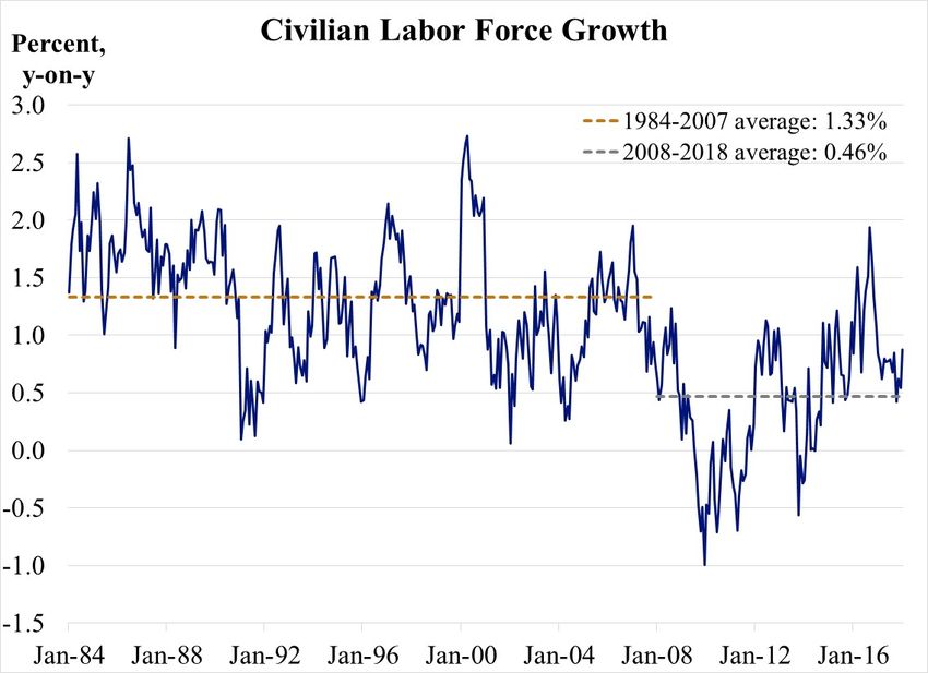
Introduction

               2
The phantom menace
•   This talk is a commentary on issues around “r*,” the natural
    real rate of interest.
•   According to leading contemporary theories, policymakers
    need to know the value of r* in order to decide if the current
    policy rate setting is accommodative, neutral or restrictive.
•   In practice, pinning down empirical values for the natural
    rate of interest involves imputing an underlying trend from
    raw data, which can be difficult.
•   Hence, this variable is something of a “phantom menace.”

                                                                     3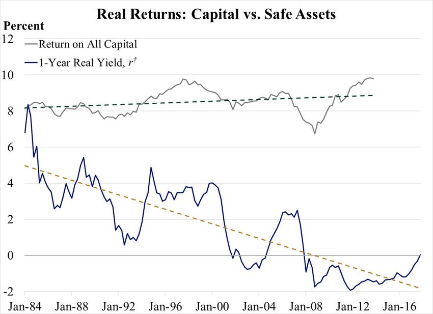
Key themes in this talk
•   The main themes in this talk are as follows:
    o r* is, in practice, a low-frequency trend measure of a short-
      term real interest rate, and this talk will take a regime-
      switching view of this issue.
    o Observed low real interest rates are associated with
      government debt, not necessarily with capital.
    o There appears to be a large demand for safe assets globally,
      and this may be the largest factor driving real interest rates to
      low levels in the past three decades.
    o There is only modest evidence that key trends influencing the
      natural rate of interest are changing today.

                                                                          4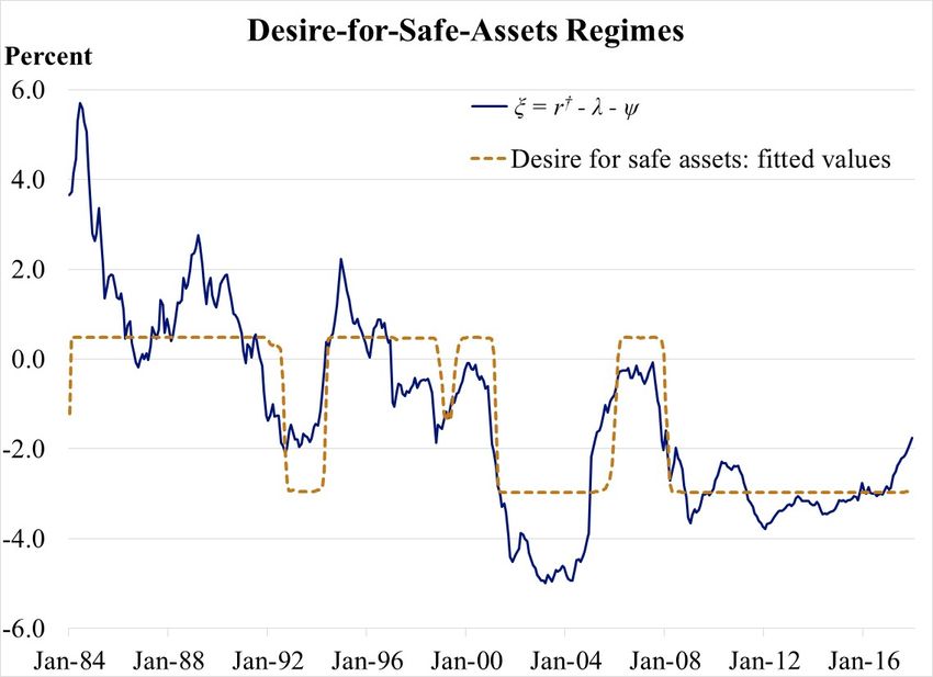
Raw Data and the Trend

                         5
Short-term real interest rates
• Short-term real interest rates are at the center of
macroeconomic theory and monetary policy.
• This talk views the natural real rate of interest as the trend
component of short-term real interest rates.
• The Fed can influence the real rate of interest but not the
trend in the real rate of interest, which is viewed as driven by
fundamental factors.
• There are many ways to detrend the data.
6Raw data
• The raw data for this talk are one-year ex-post real interest
rates on U.S. Treasury bills from 1984 to the present.1
• The following are four methods to detrend the data:
o Use a constant as in Taylor (1993).2
o Use a model, such as Holston et al. (2017) or Del Negro et al.
(2017).3
o Use a linear trend.
o Use an atheoretical filter, like the Hodrick-Prescott filter.
1 Forward-looking measures, based on the FRB of Cleveland data, are similar but more volatile.
2 J.Taylor, 1993, “Discretion versus policy rules in practice,” Carnegie-Rochester Conference Series on Public Policy, 39, pp.
195-214.
3 K. Holston, T. Laubach and J.C. Williams, 2017, “Measuring the natural rate of interest: International trends and determinants,”
Journal of International Economics, 108(S1), pp. S59-75 and M. Del Negro, D. Giannone, M.P. Giannoni and A. Tambalotti, 2017,
“Safety, Liquidity and the Natural Rate of Interest,” Brookings Papers on Economic Activity, Spring, pp. 235-303.
7Raw data with trends
Sources: Federal Reserve Board, FRB of Dallas, Taylor (1993), Del Negro et al. (2017), Holston et al. (2017) and
author’s calculations. Last observation: 2017-Q4.
8A regime-switching view
• In this talk I will give a regime-switching view of these
issues.
• Fundamental factors—mostly the same as what others have
looked at—are viewed as switching between high-mean and
low-mean states.
• I will call the natural rate of interest “r-dagger” (or r†) in
order to emphasize that these estimates use an alternative
methodology.
• To center the analysis, I will consider all issues in the
context of a Taylor-type policy rule.
• I will give the policy implications of my view at the end of
the talk.
9The Natural Rate of Interest in a
Taylor-Type Policy Rule
10Why worry about r†?
• In a Taylor-type rule, the natural real interest rate, rt† ,
determines the intercept:
it = rt† + πte + ϕπ πtGAP + ϕy ytGAP,
where πte = π* = 2 percent, the FOMC’s inflation target.
• When the gaps are zero, a Taylor-type rule simply
recommends setting the policy rate equal to the value of rt†
plus the inflation target.
• But what is the value of rt†?
11Decomposing the natural real rate
• One way to think of the natural real rate of interest is to
divide it into three factors:
rt† = λt + ψt + ξt, where
• λt: the labor productivity growth rate
• ψt: the labor force growth rate
• ξt: an investor desire for safe assets. A strong desire for
safe assets would imply a relatively large negative value
for ξt, whereas an ordinary desire for safe assets would
imply a value closer to zero.
12Why this decomposition of r†?
• Assumptions:
o log preferences T-period OLG with no discounting
o fixed capital and no other frictions
• In this type of model, if there was no special desire for safe
assets, r† would equal the real output growth rate (also the
consumption growth rate), λ + ψ, along the balanced
growth path.
• This is one concept of a natural real rate of interest.
13Longer-run outcomes as regimes
• This conception of the natural real rate of interest suggests
r† will have a constant mean associated with a single
possible balanced growth path.
• The point of this presentation is that this mean may be
better modeled as shifting over time.
• Shifting means can be modeled as regime-switching
processes.
o For example, relatively long eras of high productivity
growth may be followed by relatively long eras of low
productivity growth, and the natural real rate of interest
would be different in the two regimes.
14The declining trend is on government
paper only, not on capital
• The raw data show a declining trend on an ex-post real
return to holding government paper.
• The declining trend does not appear to extend to ex-post
real returns on claims to capital as measured from the U.S.
national accounts.
• That return has been fairly constant since the 1980s, as
shown in the next chart.
• This provides a rationale for the inclusion of the ξ factor
above, which measures the desirability of holding safe
assets relative to capital.1
1For an alternative perspective on this issue, see J.C. Williams, “Three Questions on R-star,” FRB of San Francisco
Economic Letter No. 2017-05, Feb. 21, 2017.
15Real returns on capital and safe assets
Sources: P. Gomme, B. Ravikumar and P. Rupert. “Secular Stagnation and Returns on Capital,” FRB of St. Louis Economic
Synopses No. 19, 2015; Federal Reserve Board; FRB of Dallas; and author’s calculations. Last observation: 2017-Q4.
16Main question
• Which of the three factors is most important in accounting
for the downward trend? Is it productivity growth, labor
force growth or the desirability of safe assets?
• I will treat each of these three factors as following a two-
state Markov-switching intercept process:
xt = x(st) + εt , where εt is an i.i.d. error term
st can take two values, high and low.
• The two possible mean values are called regimes.
• The idea is that these types of factors generally have
constant means, but that there can be infrequent shifts in
mean. I want to characterize these shifts statistically.
17Labor Productivity Growth
18U.S. labor productivity growth has
been low
• A statistical model that estimates the probability that the
U.S. economy is in a low-productivity-growth regime puts
nearly all the probability on the low-growth regime.1
• The most recent estimates, based on the Kahn and Rich
(2006) methodology, put the growth rate in the low (high)
state at 1.33 percent (2.90 percent).2
• The U.S. economy was in the high-productivity-growth
regime from early 1997 to late 2004.
1 See J.A. Kahn and R.W. Rich, 2006, “Tracking Productivity in Real Time,” FRB of New York, Current Issues in
Economics and Finance, 12(8).
2 In previous talks, I have used even lower productivity growth assumptions.
19The high- and low-productivity-
growth regimes
Sources: Kahn and Rich (2006) and FRB of New York. Last observation: 2017-Q4.
20Labor Force Growth
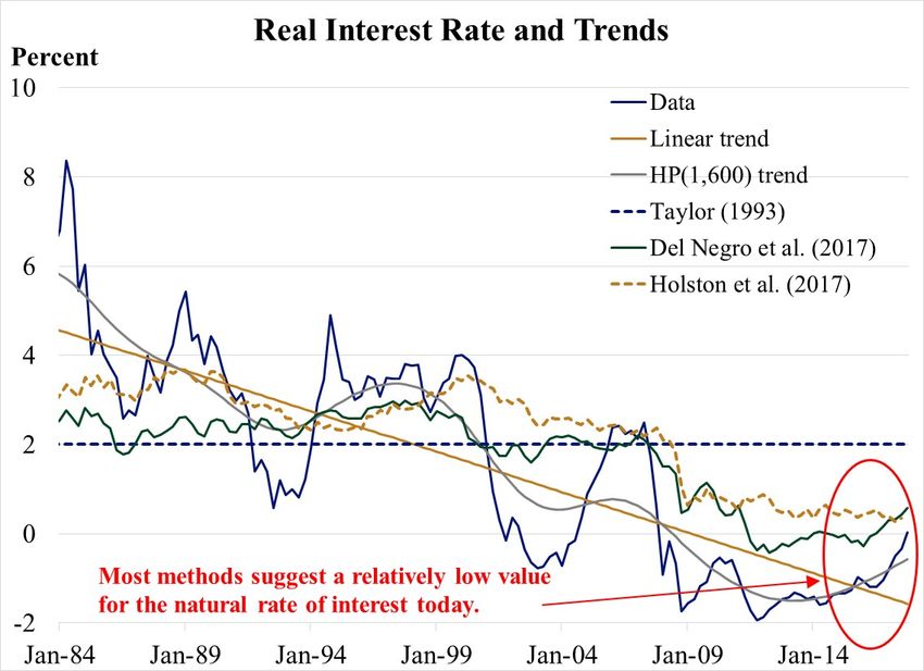
21Labor force growth has been low
• The U.S. labor force had been growing at a 1.33 percent
annual rate until the financial crisis.
• The growth rate has been 0.46 percent since the financial
crisis.
• It appears that the U.S. is in a low-growth state, but
statistically the two regimes are not precisely estimated.
• In discussing the policy implications below, I will consider
the possibility that the U.S. is in either state.
22High- and low-labor-force-growth
regimes
Sources: Bureau of Labor Statistics and author’s calculations. Last observation: January 2018.
23Investor Desire for Safe Assets
24Investor desire for safe assets
• I now remove the regime-switching trends for both labor
productivity and labor force growth from the raw data on
ex-post safe real returns.
• This leaves us with a time series of adjusted safe real
returns, and this series still has a downward trend.
• I then fit a two-state regime-switching process to these
residual values, and I interpret the two states as a strong
desire for safe assets versus a more normal desire for safe
assets.
25High-desire-for-safe-assets regime
• The estimated values for ξ are -3.06 percent in the high-
desire-for-safe-assets regime and 0.57 percent in the
normal-desire-for-safe-assets regime.
• The U.S. is currently in the regime with a high desire for
safe assets.
• The difference between the two regimes is largest for this
factor; in some sense, it is the “most important” of the
three.
26Current regime: High desire for safe
assets
Source: Author’s calculations. Last observation: December 2017.
27What Does This Imply for the Natural Real
Rate of Interest?
28State values for each factor
High-low
High Low
Factor state
state state
difference
Labor productivity growth, λ 290 133 157
Labor force growth, ψ 133 46 87
Investor desire for safe assets 57 -306 363
(inverse), ξ
Max/min natural rate, r† 480 -127 607
All values are expressed as basis points. The max (min) natural rate is the value corresponding to all three factors taking
the value in the high (low) state.
29Using the regime-switching approach
• Labor productivity appears to be in the low-growth
regime, so set λ = 1.33 percent.
• The labor force appears to be in the low-growth regime as
well, so set ψ = 0.46 percent. Plausibly, labor force
growth could be interpreted as still consistent with the
high-growth regime, ψ = 1.33 percent.
• There also appears to be a high desire for safe assets, so set
ξ = -3.06 percent.
• According to this analysis, r† = λ + ψ + ξ is either -127
basis points or -40 basis points, depending on how one
views labor force growth.
30Recent Related Estimates
from the Literature
31Related literature and regime
switching
• There is a fairly large and growing literature trying to
understand the downward trend in the natural real rate of
interest.
• The literature tends to be quite a bit more sophisticated than
the analysis presented here.
• The only point here is to think in terms of regime switching.
• Two of the three factors analyzed—labor productivity
growth and the desire for safe assets—are in the low state
and do not appear to be shifting to the high state.
• This suggests the natural safe real rate of interest, and hence
the Fed’s policy rate, can remain low over the forecast
horizon.
32Related literature on the natural rate
• Laubach and Williams (2003) impose a structural model and
estimate a relatively low r*.1
o Holston et al. (2017) extend the analysis to other countries.
• Curdia (2015) performs a similar analysis with somewhat
altered assumptions and gets a very low r*.2
• Del Negro et al. (2017) impose a structural model, include an
evolving demand for safe assets and get a low value for r*.
• I have imposed less structure along with an alternative
stochastic conception, regime switching. This suggests a
different view of mean-reversion properties.
1 T. Laubach and J.C. Williams, “Measuring the Natural Rate of Interest,” Review of Economics and Statistics,
November 2003, 85(4), 1063–70.
2 V. Curdia, “Why So Slow? A Gradual Return for Interest Rates,” FRB of San Francisco Economic Letter No. 2015-32,
Oct. 12, 2015.
33Additional related literature
• More possible factors impacting real rates are analyzed in
Rachel and Smith (2015).1
• One could also take a longer-run view of the natural safe real
rate of interest.
o Borio et al. (2017) consider a panel dataset for 19 countries
from 1870 to the present.2 Their analysis emphasizes
monetary regimes over long eras.
• Even more data: Homer and Sylla (2005).3
1 L. Rachel and T.D. Smith, “Secular drivers of the global real interest rate,” Bank of England Staff Working Paper No.
571, December 2015.
2 C. Borio, P. Disyatat, M. Juselius and P. Rungcharoenkitkul “Why so low for so long? A long-term view of real interest
rates,” Bank for International Settlements Working Papers No. 685, December 2017.
3 S. Homer and R. Sylla, A History of Interest Rates, Fourth Edition, John Wiley & Sons Inc., 2005.
34Implications for the
Policy Rate
35Implications for monetary policy
• I now return to a Taylor-type monetary policy rule to give
some sense of the policy impact of this analysis.
• As I noted earlier, if the gaps in a Taylor-type rule are
viewed as close to zero, the rule would recommend a policy
rate setting equal to the natural rate plus the inflation target.
• The gap variables are probably not exactly zero today, so I
now turn to a brief discussion of the values for gap variables.
36The inflation gap
• The U.S. inflation rate has been below the 2 percent
inflation target since 2012.*
• Inflation measured from one year earlier is currently
(December 2017) between 30 and 48 basis points below
target:
o Dallas Fed trimmed-mean PCE 1.67%
o Headline PCE 1.70%
o Core PCE 1.52%
* The inflation target is in terms of the annual change in the price index for personal consumption expenditures (PCE).
37The output gap
• I look at three ways to calculate an output gap.
• The CBO output gap (2017-Q4): 0.47 percent
• The deviation from HP1,600 trend (2017-Q4): 0.14 percent
• Okun’s law implied gap: 0.92 percent
o St. Louis Fed’s “no-recession regime” estimate: u* = 4.5 percent
o Unemployment rate (January 2018): u = 4.1 percent
o Output gap: 2.3*(4.5 – 4.1) = 0.92 percent
38Data summary and two policy rules
• I consider two Taylor-type rules:1
i = r† + π e + ϕπ π GAP + ϕy y GAP
1. Taylor (1993): ϕπ = 1.5, ϕy = 0.5
2. Taylor (1999):2 ϕπ = 1.5, ϕy = 1
o Inflation target: π e = π* = 200
o Natural real rate: r† ∈ [-127, -40]
o The inflation gap: π GAP ∈ [-48, -30]
o The output gap: y GAP ∈ [14, 92]
1All values in these calculations are expressed as basis points.
2J. Taylor, “A Historical Analysis of Monetary Policy Rules,” in J. Taylor, ed., Monetary Policy Rules, University of
Chicago Press, ch. 7, pp. 319-48, 1999.
39Policy rate recommendations
• Based on these data and rules, then the policy rate i should
be set as:
1. Taylor (1993) implies i ∈ [8, 161].
2. Taylor (1999) implies i ∈ [15, 207].
• The FOMC’s target range for the federal funds rate today is
125 to 150 basis points, and the federal funds rate is trading
at about 142 basis points.
• This value is within the range of the recommendations.
• However, if the Committee raises the policy rate
substantially from here without other changes in the data, the
policy setting could become restrictive.
40Mean-reversion properties
• The regime-switching approach suggests that the current
setting of the policy rate is broadly appropriate.
• It also suggests that r† is unlikely to shift over a forecast
horizon of two years (the typical time frame for monetary
policy decisions).
• This suggests forward guidance should be characterized by
a relatively flat policy rate path, as opposed to an upward-
sloping one that would be appropriate if r† has strong mean
reversion.
41Conclusion
42Conclusions
• This analysis has provided some background on how one
might begin to think about recent trends in the natural safe
real rate of interest in a regime-switching context.
• According to the analysis presented here, the natural safe
real rate of interest, and hence the appropriate policy rate,
is relatively low and unlikely to change very much over the
forecast horizon.
• A more rigorous and thorough analysis that reaches a
similar conclusion is Del Negro et al. (2017).
43Connect With Us
James Bullard
stlouisfed.org/from-the-president
STLOUISFED.ORG
Federal Reserve Blogs and Economic Community
Economic Data Publications Education Development
(FRED) News and views Resources Promoting financial
Thousands of data about the economy For every stage stability of families,
series, millions of users and the Fed of life neighborhoods
SOCIAL MEDIA ECONOMY MUSEUM
44You can also read