Real-Time Stochastic Optimal Control for Multi-agent Quadrotor Systems
←
→
Page content transcription
If your browser does not render page correctly, please read the page content below
Real-Time Stochastic Optimal Control for Multi-agent Quadrotor Systems
                                                 Vicenç Gómez1 , Sep Thijssen2 , Andrew Symington3 , Stephen Hailes4 , Hilbert J. Kappen2
                                                                       1
                                                                         Universitat Pompeu Fabra. Barcelona, Spain vicen.gomez@upf.edu
                                                        2
                                                            Radboud University Nijmegen, the Netherlands {s.thijssen,b.kappen}@donders.ru.nl
                                                                 3
                                                                   University of California Los Angeles, USA andrew.c.symington@gmail.com
                                                                     4
                                                                       University College London, United Kingdom s.hailes@cs.ucl.ac.uk
arXiv:1502.04548v6 [eess.SY] 12 May 2020

                                                                       Abstract
                                             This paper presents a novel method for controlling teams
                                             of unmanned aerial vehicles using Stochastic Optimal Con-
                                             trol (SOC) theory. The approach consists of a centralized
                                             high-level planner that computes optimal state trajectories as
                                             velocity sequences, and a platform-specific low-level con-
                                             troller which ensures that these velocity sequences are met.
                                             The planning task is expressed as a centralized path-integral
                                             control problem, for which optimal control computation cor-
                                             responds to a probabilistic inference problem that can be
                                             solved by efficient sampling methods. Through simulation
                                             we show that our SOC approach (a) has significant benefits
                                             compared to deterministic control and other SOC methods
                                             in multimodal problems with noise-dependent optimal solu-
                                             tions, (b) is capable of controlling a large number of platforms
                                             in real-time, and (c) yields collective emergent behaviour in
                                             the form of flight formations. Finally, we show that our ap-
                                             proach works for real platforms, by controlling a team of
                                             three quadrotors in outdoor conditions.

                                                                1     Introduction
                                           The recent surge in autonomous Unmanned Aerial Vehicle
                                           (UAV) research has been driven by the ease with which plat-          Figure 1: Control hierarchy: The path-integral controller
                                           forms can now be acquired, evolving legislation that reg-            (1) calculates target velocities/heights for each quadrotor.
                                           ulates their use, and the broad range of applications en-            These are converted to roll, pitch, throttle and yaw rates by
                                           abled by both individual platforms and cooperative swarms.           a platform-specific Velocity Height PID controller (2). This
                                           Example applications include automated delivery systems,             control is in turn passed to the platform’s flight control sys-
                                           monitoring and surveillance, target tracking, disaster man-          tem (3), and converted to relative motor speed changes.
                                           agement and navigation in areas inaccessible to humans.
                                              Quadrotors are a natural choice for an experimental plat-
                                           form, as they provide a safe, highly-agile and inexpensive           case, for which a closed form solution exists, solving the
                                           means by which to evaluate UAV controllers. Figure 1 shows           SOC problem requires solving the Hamilton Jacobi Bellman
                                           a 3D model of one such quadrotor, the Ascending Technolo-            (HJB) equations. These equations are generally intractable,
                                           gies Pelican. Quadrotors have non-linear dynamics and are            and so the SOC problem remains an open challenge.
                                           naturally unstable, making control a non-trivial problem.
                                                                                                                   In such a complex setting, a hierarchical approach is usu-
                                              Stochastic optimal control (SOC) provides a promising
                                                                                                                ally taken and the control problem is reduced to follow a
                                           theoretical framework for achieving autonomous control of
                                                                                                                state-trajectory (or a set of way points) designed by hand
                                           quadrotor systems. In contrast to deterministic control, SOC
                                                                                                                or computed offline using trajectory planning algorithms
                                           directly captures the uncertainty typically present in noisy
                                                                                                                (Kendoul 2012). While the planning step typically involves
                                           environments and leads to solutions that qualitatively de-
                                                                                                                a low-dimensional state representation, the control methods
                                           pend on the level of uncertainty (Kappen 2005). However,
                                                                                                                use a detailed complex state representation of the UAV. Ex-
                                           with the exception of the simple Linear Quadratic Gaussian
                                                                                                                amples of control methods for trajectory tracking are the
                                           Copyright c 2016, Association for the Advancement of Artificial      Proportional Integral Derivative or the Linear-Quadratic reg-
                                           Intelligence (www.aaai.org). All rights reserved.                    ulator.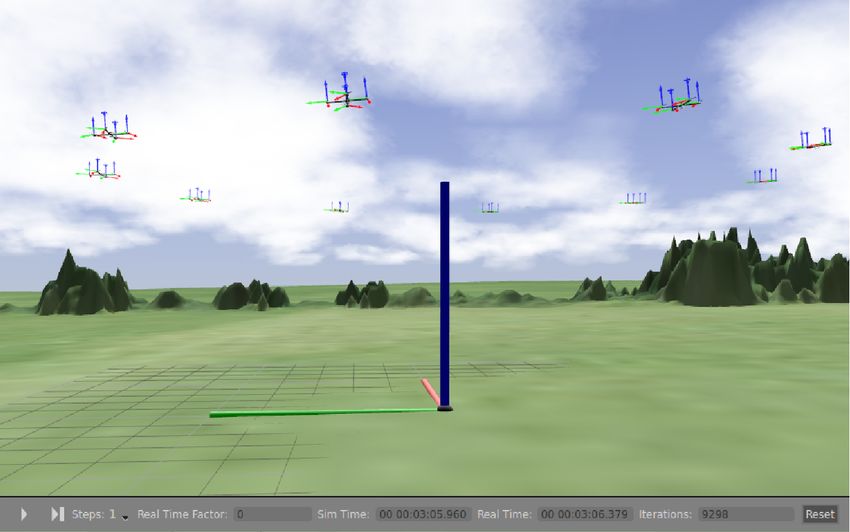
A generic class of SOC problems was introduced in Kap-        an optimal control problem at time t and state x(t) over a
pen; Todorov (2005; 2006) for which the controls and the         future horizon of a fixed number of time-steps. The first op-
cost function are restricted in a way that makes the HJB         timal move u∗ (t) is then applied and the rest of the optimal
equation linear and therefore more efficiently solvable. This    sequence is discarded. The process is repeated again at time
class of problems is known as path integral (PI) control,        t + 1. A quadratic cost function is typically used, but other
linearly-solvable controlled diffusions or Kullback-Leibler      more complex functions exist.
control, and it has lead to successful robotic applications,        MPC has mostly been used in indoor scenarios, where
e.g. (Kinjo, Uchibe, and Doya 2013; Rombokas et al. 2012;        high-precision motion capture systems are available. For in-
Theodorou, Buchli, and Schaal 2010). A particularly inter-       stance, in Kushleyev et al. (2013) authors generate smooth
esting feature of this class of problems is that the compu-      trajectories through known 3-D environments satisfying
tation of optimal control is an inference problem with a so-     specifications on intermediate waypoints and show remark-
lution given in terms of the passive dynamics. In a multi-       able success controlling a team of 20 quadrotors. Trajectory
agent system, where the agents follow independent passive        optimization is translated to a relaxation of a mixed inte-
dynamics, such a feature can be exploited using approxi-         ger quadratic program problem with additional constraints
mate inference methods such as variational approximations        for collision avoidance, that can be solved efficiently in real-
or belief propagation (Kappen, Gómez, and Opper 2012;           time. Examples that follow a similar methodology can be
Van Den Broek, Wiegerinck, and Kappen 2008).                     found in Turpin, Michael, and Kumar; Augugliaro, Schoel-
   In this paper, we show how PI control can be used for         lig, and D’Andrea (2012; 2012). Similarly to our approach,
solving motion planning tasks on a team of quadrotors in         these methods use a simplified model of dynamics, either us-
real time. We combine periodic re-planning with receding         ing the 3-D position and yaw angle Kushleyev et al.; Turpin,
horizon, similarly to model predictive control, with effi-       Michael, and Kumar (2013; 2012) or the position and ve-
cient importance sampling. At a high level, each quadro-         locities as in Augugliaro, Schoellig, and D’Andrea (2012).
tor is modelled as a point mass that follows simple dou-         However, these approaches are inherently deterministic and
ble integrator dynamics. Low-level control is achieved us-       express the optimal control problem as a quadratic problem.
ing a standard Proportional Integral Derivative (PID) veloc-     In our case, we solve an inference problem by sampling and
ity controller that interacts with a real or simulated flight    we do not require intermediate trajectory waypoints.
control system. With this strategy we can scale PI control to       In outdoor conditions, motion capture is difficult and
ten units in simulation. Although in principle there are no      Global Positioning System (GPS) is used instead. Existing
further limits to experiments with actual platforms, our first   control approaches are typically either based on Reynolds
results with real quadrotors only include three units. To the    flocking (Bürkle, Segor, and Kollmann 2011; Hauert et al.
best of our knowledge this has been the first real-time im-      2011; Vásárhelyi et al. 2014; Reynolds 1987) or flight for-
plementation of PI control on an actual multi-agent system.      mation (Guerrero and Lozano 2012; Yu et al. 2013). In
   In the next section we describe related work. We introduce    Reynolds flocking, each agent is considered a point mass
our approach in Section 3 Results are shown on three dif-        that obeys simple and distributed rules: separate from neigh-
ferent scenarios in Section 4 Finally, Section 5 concludes       bors, align with the average heading of neighbors and steer
this paper.                                                      towards neighborhood centroid to keep cohesion. Flight for-
                                                                 mation control is typically modeled using graphs, where ev-
    2    Related Work on UAV Planning and                        ery node is an agent that can exchange information with all
                     Control                                     or several agents. Velocity and/or position coordination is
                                                                 usually achieved using consensus algorithms.
There is a large and growing body of literature related to          The work in Quintero, Collins, and Hespanha (2013)
this topic. In this section, we highlight some of the most       shares many similarities with our approach. Authors derive a
related papers to the presented approach. An recent sur-         stochastic optimal control formulation of the flocking prob-
vey of control methods for general UAVs can be found             lem for fixed-wings UAVs. They take a leader-follower strat-
in Kendoul (2012).                                               egy, where the leader follows an arbitrary (predefined) pol-
   Stochastic optimal control is mostly used for UAV con-        icy that is learned offline and define the immediate cost as
trol in its simplest form, assuming a linear model perturbed     a function of the distance and heading with respect to the
by additive Gaussian noise and subject to quadratic costs        leader. Their method is demonstrated outdoors with 3 fixed-
(LQG), e.g. (How et al. 2008). While LQG can successfully        wing UAVs in a distributed sensing task. As in this paper,
perform simple actions like hovering, executing more com-        they formulate a SOC problem and perform MPC. However,
plex actions requires considering additional corrections for     in our case we do not restrict to a leader-follower setup and
aerodynamic effects such as induced power or blade flap-         consider a more general class of SOC problems which can
ping (Hoffmann et al. 2011). These approaches are mainly         include coordination and cooperation problems.
designed for accurate trajectory control and assume a given
desired state trajectory that the controller transforms into     Planning approaches Within the planning community,
motor commands.                                                  Bernardini, Fox, and Long (2014) consider search and track-
   Model Predictive Control (MPC) has been used optimize         ing tasks, similar to one of our scenarios. Their approach
trajectories in multi-agent UAV systems (Shim, Kim, and          is different to ours, they formulate a planning problem that
Sastry 2003). MPC employs a model of the UAV and solves          uses used search patterns that must be selected and se-
quenced to maximise the probability of rediscovering the bitrary functions, f is the drift in the uncontrolled dynamics
target. Albore et al. (2015) and Chanel, Teichteil-Knigsbuch, (including gravity, Coriolis and centripetal forces), and G
and Lesire (2013) consider a different problem: dynamic describes the effect of the control u into the state vector x.
data acquisition and environmental knowledge optimisation. A realization τ = x0:dt:T of the above equation is called
Both techniques use some form of replanning. While Al- a (random) path. In order to describe a control problem we
bore et al. (2015) uses a Markov Random Field framework define the cost that is attributed to a path (cost-to-go) by
to represent knowledge about the uncertain map and its qual-
ity, Chanel, Teichteil-Knigsbuch, and Lesire (2013) rely on S(τ |x0 , u) = rT (xT )
partially-observable MDPs. All these works consider a sin- X 1 >
gle UAV scenario and low-level control is either neglected + rt (xt ) + ut Rut dt, (2)
2
t=0:dt:T −dt
or deferred to a PID or waypoint controller.
Recent Progress in Path-Integral Control There has where rT (xT ) and rt (xt ) are arbitrary state cost terms at
been significant progress in PI control, both theoretically and end and intermediate times, respectively. R is the control
in applications. Most of existing methods use parametrized cost matrix. The general stochastic optimal control problem
policies to overcome the main limitations (see Section 3.1). is to minimize the expected cost-to-go w.r.t. the control
Examples can be found in Theodorou, Buchli, and Schaal; u∗ = arg min E[S(τ |x0 , u)].
Stulp and Sigaud; Gómez et al. (2010; 2012; 2014). In u
these methods, the optimal control solution is restricted by In general, such a minimization leads to the Hamilton-
the class of parametrized policies and, more importantly, Jacobi-Bellman (HJB) equations, which are non-linear, sec-
it is computed offline. In Rawlik, Toussaint, and Vijayaku- ond order partial differential equations. However, under the
mar (2013), authors propose to approximate the transformed following relation between the control cost and noise co-
cost-to-go function using linear operators in a reproducing variance Σu = λR−1 , the resulting equation is linear in the
kernel Hilbert space. Such an approach requires an analyt- exponentially transformed cost-to-go function. The solution
ical form of the PI embedding, which is difficult to obtain is given by the Feynman-Kac Formula, which expresses op-
in general. In Horowitz, Damle, and Burdick (2014), a low- timal control in terms of a Path-Integral, which can be in-
rank tensor representation is used to represent the model dy- terpreted as taking the expectation under the optimal path
namics, allowing to scale PI control up to a 12-dimensional distribution (Kappen 2005)
system. More recently, the issue of state-dependence of the
optimal control has been addressed (Thijssen and Kappen p∗ (τ |x0 ) ∝ p(τ |x0 , u) exp(−S(τ |x0 , u)/λ), (3)
2015), where a parametrized state-dependent feedback con- hu∗t (x0 )i = hut + (ξt+dt − ξt )/dti , (4)
troller is derived for the PI control class.
Finally, model predictive PI control has been recently pro- where p(τ |x0 , u) denotes the probability of a (sub-optimal)
posed for controlling a nano-quadrotor in indoor settings path under equation (1) and h·i denotes expectation over
in an obstacle avoidance task (Williams, Rombokas, and paths distributed by p∗ .
Daniel 2014). In contrast to our approach, their method is The constraint Σu = λR−1 forces control and noise to act
not hierachical and uses naive sampling, which makes it less in the same dimensions, but in an inverse relation. Thus, for
sample efficient. Additionally, the control cost term is ne- fixed λ, the larger the noise, the cheaper the control and vice-
glected, which can have important implications in complex versa. Parameter λ act as a temperature: higher values of λ
tasks involving noise. The approach presented here scales result in optimal solutions that are closer to the uncontrolled
well to several UAVs in outdoor conditions and is illustrated process.
in tasks beyond obstacle avoidance navigation. Equation (4) permits optimal control to be calculated by
probabilistic inference methods, e.g., Monte Carlo. An in-
teresting fact is that equations (3, 4) hold for all controls
3 Path-Integral Control for Multi-UAV u. In particular, u can be chosen to reduce the variance in
planning the Monte Carlo computation of hu∗t (x0 )i which amounts
We first briefly review PI control theory. This is followed by to importance sampling. This technique can drastically im-
a description of the proposed method used to achieve motion prove the sampling efficiency, which is crucial in high di-
planning of multi-agent UAV systems using PI control. mensional systems. Despite this improvement, direct appli-
cation of PI control into real systems is limited because it is
3.1 Path-Integral Control not clear how to choose a proper importance sampling dis-
We consider continuous time stochastic control problems, tribution. Furthermore, note that equation (4) yields the op-
where the dynamics and cost are respectively linear and timal control for all times t averaged over states. The result
quadratic in the control input, but arbitrary in the state. is therefore an open-loop controller that neglects the state-
More precisely, consider the following stochastic differential dependence of the control beyond the initial state.
equation of the state vector x ∈ Rn under controls u ∈ Rm
3.2 Multi-UAV planning
dx = f (x)dt + G(x)(udt + dξ), (1)
The proposed architecture is composed of two main levels.
where ξ is m−dimensional Wiener noise with covariance At the most abstract level, the UAV is modeled as a 2D
Σu ∈ Rm×m and f (x) ∈ Rn and G(x) ∈ Rn×m are ar- point-mass system that follows double integrator dynamics.Algorithm 1 PI control for UAV motion planning
1: function PIC ONTROLLER(N, H, dt, rt (·), Σu , ut:dt:t+H )
2: for k = 1, . . . , N do
3: Sample paths τk = {xt:dt:t+H }k with Eq. (5)
4: end for
5: Compute Sk = S(τk |x0 , u) with Eq. (2)
6: Store the noise realizations {ξt:dt:t+H P}k
7: Compute the weights: wk = e−Sk /λ / l e−Sl /λ
8: for s = t : dt : t +P H do
9: u∗s = us + dt 1
k wk ({ξs+dt }k − {ξs }k )
10: end for
11: Return next desired velocity: vt+dt = vt + u∗t dt Figure 2: The flight control system (FCS) is comprised of
and u∗t:dt:t+H for importance sampling at t + dt two control loops: one for stabilization and the other for pose
12: end function control. A low-level controller interacts with the FCS over a
serial interface to stream measurements and issue control.
At the low-level, we use a detailed second order model that
we learn from real flight data (De Nardi and Holland 2008). dimension-independent, i.e. Σu = σu2 Id. To measure sam-
We use model predictive control combined with importance pling convergence, we define the Effective Sample Size
PN
sampling. There are two main benefits of using the proposed (ESS) as ESS := 1/ k=1 wk2 , which is a quantity between
approach: first, since the state is continuously updated, the 1 and N . Values of ESS close to one indicate an estimate
controller does not suffer from the problems caused by us- dominated by just one sample and a poor estimate of the
ing an open-loop controller. Second, the control policy is not optimal control, whereas an ESS close to N indicates near
restricted by any parametrization. perfect sampling, which occurs when the importance- equals
The two-level approach permits to transmit control sig- the optimal-control function.
nals from the high-level PI controller to the low-level control
system at a relatively low frequencies (we use 15Hz in this 3.3 Low Level Control
work). Consequently, the PI controller has more time avail- >
The target velocity v = [vE vN ] is passed along with
able for sampling a large number of trajectories, which is a height p̂U to a Velocity-Height controller. This con-
critical to obtain good estimates of the control. The choice of troller uses the current state estimate of the real quadrotor
2D in the presented method is not a fundamental limitation, >
as long as double-integrator dynamics is used. The control y = [pE pN pU φ θ ψ u v w p q r] , where (pE , pN , pU )
hierarchy introduces additional model mismatch. However, and (φ, θ, ψ) denote navigation-frame position and orienta-
as we show in the results later, this mismatch is not critical tion and (u, v, w), (p, q, r) denote body-frame and angular
for obtaining good performance in real conditions. velocities, respectively. It is composed of four independent
Ignoring height, the state vector x is thus composed of the PID controllers for roll φ̂, pitch θ̂, throttle γ̂ and yaw rate r̂.
East-North (EN) positions and EN velocities of each agent that send the commands to the flight control system (FCS)
i = 1, . . . , M as xi = [pi , vi ]> where pi , vi ∈ R2 . Similarly, to achieve v.
the control u consists of EN accelerations ui ∈ R2 . Equa- Figure 2 shows the details of the FCS. The control loop
tion (1) decouples between the agents and takes the linear runs at 1kHz fusing triaxial gyroscope, accelerometer and
form magnetometer measurements. The accelerometer and mag-
netometer measurements are used to determine a reference
dxi = Axi dt + B(ui dt + dξi ), global orientation, which is in turn used to track the gyro-
0 1
0 scope bias. The difference between the desired and actual
A= , B= . (5) angular rates are converted to motor speeds using the model
0 0 1
in Mahony, Kumar, and Corke (2012).
Notice that although the dynamics is decoupled and linear, An outer pose control loop calculates the desired angular
the state cost rt (xt ) in equation (2) can be any arbitrary rates based on the desired state. Orientation is obtained from
function of all UAVs states. As a result, the optimal con- the inner control loop, while position and velocity are ob-
trol will in general be a non-linear function that couples all tained by fusing GPS navigation fixes with barometric pres-
the states and thus hard to compute. sure (BAR) based altitude measurements. The radio trans-
Given the current joint optimal action u∗t and velocity mitter (marked TX in the diagram) allows the operator to
vt , the expected velocity at the next time t0 is calculated as switch quickly between autonomous and manual control of
vt0 = vt + (t0 − t)u∗t and passed to the low-level controller. a platform. There is also an acoustic alarm on the platform
The final algorithm optionally keeps an importance-control itself, which warns the operator when the GPS signal is lost
sequence ut:dt:t+H that is incrementally updated. We sum- or the battery is getting low. If the battery reaches a critical
marize the high-level controller in Algorithm 1. level or communication with the transmitter is lost, the plat-
The importance-control sequence ut:dt:t+H is initialized form can be configured to land immediately or alternatively,
using prior knowledge or with zeros otherwise. Noise is to fly back and land at its take-off point.horizon problem. A key difference between iLQG and PI
control is that the linear-quadratic approximation is certainty
equivalent. Consequently, iLQG yields a noise independent
solution.
4.1 Scenario I: Drunken Quadrotor
This scenario is inspired in Kappen (2005) and highlights the
benefits of SOC in a quadrotor task. The Drunken Quadro-
tor is a finite horizon task where a quadrotor has to reach a
target, while avoiding a building and a wall (figure 3). There
are two possible routes: a shorter one that passes through a
small gap between the wall and the building, and a longer
Figure 3: Drunken Quadrotor: a red target has to be reached one that goes around the building. Unlike SOC, the deter-
while avoiding obstacles. (Left) the shortest route is the op- ministic optimal solution does not depend on the noise level
timal solution in the absence of noise. (Right) with control and will always take the shorter route. However, with added
noise, the optimal solution is to fly around the building. noise, the risk of collision increases and thus the optimal
noisy control is to take the longer route.
This task can be alternatively addressed using other plan-
3.4 Simulator Platform ning methods, such as the one proposed by Ono, Williams,
We have developed an open-source framework called and Blackmore (2013), which allow for specification of
CRATES1 . The framework is a implementation of QRSim user’s acceptable levels of risk using chance constraints.
(De Nardi 2013; Symington et al. 2014) in Gazebo, which Here we focus on comparing deterministic and stochastic
uses Robot Operating System (ROS) for high-level control. optimal control for motion planning. The amount of noise
It permits high-level controllers to be platform-agnostic. It is thus determines whether the optimal solution is go through
similar to the Hector Quadrotor project (Meyer et al. 2012) the risky path or the longer safer path.
with a formalized notion of a hardware abstraction layers. The state cost in this problem consists of hard constraints
The CRATES simulator propagates the quadrotor state that assign infinite cost when either the wall or the build-
forward in time based on a second order model (De Nardi ing is hit. PI control deals with collisions by killing par-
and Holland 2008). The equations were learned from real ticles that hit the obstacles during Monte Carlo sampling.
flight data and verified by expert domain knowledge. In ad- For iLQG, the local approximations require a twice differ-
dition to platform dynamics, CRATES also simulates var- entiable cost function. We resolved this issue by adding a
ious noise-perturbed sensors, wind shear and turbulence. smooth obstacle-proximity penalty in the cost function. Al-
Orientation and barometric altitude errors follow zero-mean though iLQG computes linear feedback, we tried to improve
Ornstein-Uhlenbeck processes, while GPS error is modeled it with a MPC scheme, similar as for PI control. Unfortu-
at the pseudo range level using trace data available from nately, this leads to numerical instabilities in this task, since
the International GPS Service. In accordance with the Mil- the system disturbances tend to move the reference trajec-
itary Specification MIL-F-8785C, wind shear is modeled as tory through a building when moving from one time step to
a function of altitude, while turbulence is modeled as a dis- the next. For MPC with PI control we use a receding horizon
crete implementation of the Dryden model. CRATES also of three seconds and perform re-planning at a frequency of
provides support for generating terrain from satellite images 15 Hz with N = 2000 sample paths. Both methods are ini-
and light detection and ranging (LIDAR) technology, and tialized with ut = 0, ∀t. iLQG requires approximately 103
reporting collisions between platforms and terrain. iterations to converge with a learning rate of 0.5%.
Figure 3 (left) shows an example of real trajectory com-
4 Results puted for low control noise level, σu2 = 10−3 . To be able
to obtain such a trajectory we deactivate sensor uncertain-
We now analyze the performance of the proposed approach
ties in accelerometer, gyroscope, orientation and altimeter.
in three different tasks. We first show that, in the presence of
External noise is thus limited to aerodynamic turbulences
control noise, PI control is preferable over other approaches.
only. In this case, both iLQG and PI solutions correspond to
For clarity, this scenario is presented for one agent only. We
the shortest path, i.e. go through the gap between the wall
then consider two tasks involving several units: a flight for-
and the building. Figure 3 (right) illustrates the solutions ob-
mation task and a pursuit-evasion task.
tained for larger noise level σu2 = 1. While the optimal ref-
We compare the PI control method described in Section
erence trajectory obtained by iLQG does not change, which
3.2 with iterative linear-quadratic Gaussian (iLQG) control
results in collision once the real noisy controller is executed
(Todorov and Li 2005). iLQG is a state-of-the-art method
(left path), the PI control solution avoids the building and
based on differential dynamic programming, that iteratively
takes the longer route (right path). Note that iLQG can find
computes local linear-quadratic approximations to the finite
both solutions depending on initialization. However, How-
1
CRATES stands for ’Cognitive Robotics Architecture for ever, it will always choose the shortest route, regardless of
Tightly-Coupled Experiments and Simulation’. Available at nearby obstacles. Also, note that the PI controlled unit takes
https://bitbucket.org/vicengomez/crates a longer route to reach the target. The reason is that the con-90 1
iLQG
PI
0.8
Percent of crashes
80
Cost solution
0.6
70
0.4
60
0.2
50 0
0 0.05 0.1 0.15 0.2 0 0.05 0.1 0.15 0.2
Wind velocity (m/s) Wind velocity (m/s)
Figure 4: Results: Drunken Quadrotor with wind: For different wind velocities and fixed control noise σu2 = 0.5. (Left) cost
of the obtained solutions and (Right) percentage of crashes using iLQG and PI.
trol cost R is set quite high in order to reach a good ESS.
Alternatively, if R is decreased, the optimal solution could
reach the target sooner, but at the cost of a decreased ESS.
This trade-off, which is inherent in PI control, can be re-
solved by incorporating feedback control in the importance
sampling, as presented in Thijssen and Kappen (2015).
We also consider more realistic conditions with noise not
limited to act in the control. Figure 4 (a,b) shows results in
the presence of wind and sensor uncertainty. Panel (a) shows
how the wind affects the quality of the solution, resulting in
an increase of the variance and the cost for stronger wind.
In all our tests, iLQG is not able to bring the quadrotor to
the other side. Panel (b) shows the percentage of crashes
using both methods. Crashes occur often using iLQG con-
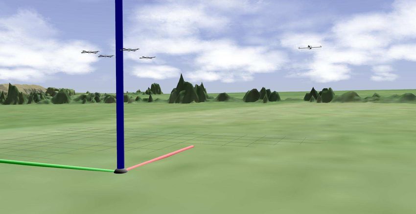
trol and only occasionally using PI control. With stronger Figure 5: Holding pattern in the CRATES simulator. Ten
wind, the iLQG controlled unit does occasionally not even units coordinate their flight in a circular formation. In this
reach the corridor (the unit did not reach the other side but example, N = 104 samples, control noise is σu2 = 0.1 and
did not crash either). This explains the difference in percent- horizon H = 1 sec. Cost parameters are vmin = 1, vmax =
ages of Panel (b). We conclude that for multi-modal tasks 3, Chit = 20 and d = 7. Environmental noise and sensing
(tasks where multiple solution trajectories exist), the pro- uncertainties are modeled using realistic parameter values.
posed method is preferable to iLQG.
4.2 Scenario II: Holding Pattern where vmax and vmin denote the maximum and minimum ve-
The second scenario addresses the problem of coordinating locities, respectively, d denotes penalty for deviation from
agents to hold their position near a point of interest while the origin and Chit is the penalty for collision risk of two
keeping a safe range of velocities and avoiding crashing into agents. k · k2 denotes `-2 norm.
each other. Such a problem arises for instance when multiple The optimal solution for this problem is a circular flying
aircraft need to land at the same location, and simultaneous pattern where units fly equidistantly from each other. The
landing is not possible. The resulting flight formation has value of parameter d determines the radius and the average
been used frequently in the literature (Vásárhelyi et al. 2014; velocities of the agents are determined from vmin and vmax .
How et al. 2008; Yu et al. 2013; Franchi et al. 2012), but Since the solution is symmetric with respect to the direc-
always with prior specification of the trajectories. We show tion of rotation (clockwise or anti-clockwise), only when the
how this formation is obtained as the optimal solution of a control is executed, a choice is made and the symmetry is
SOC problem. broken. Figure 5 shows a snapshot of a simulation after the
Consider the following state cost (omitting time indexes) flight formation has been reached for a particular choice of
parameter values 2 . Since we use an uninformed initial con-
M
X trol trajectory, there is a transient period during which the
rHP (x) = exp (vi − vmax ) + exp (vmin − vi ) agents organize to reach the optimal configuration. The co-
i=1 ordinated circular pattern is obtained regardless of the initial
M positions. This behavior is robust and obtained for a large
range of parameter values.
X
+ exp (k pi − d k2 ) + Chit / k pi − pj k2
j>i 2
Supplementary video material is available at http://www.
(6) mbfys.ru.nl/staff/v.gomez/uav.html(a) (b) (c) (d)
3
450 250 1.1 10
N=10 2
N=10
400 N=102 N=104
3
N=10
200 1.05
350 2
10
Cost iLQG/PI
state cost
state cost
300
ESS
150 1
250
1
10
200
100 0.95
150
0
100 50 0.9 10
0 50 100 150 2 4 6 8 10 −3 −2 −1 −3 −2 −1 0
10 10 10 10 10 10 10
time number of quadrotors Noise level σ2 Noise level σ2
u u
Figure 6: Holding pattern: (a) evolution of the state cost for different number of samples N = 10, 102 , 103 . (b) scaling of the
method with the number of agents. For different control noise levels, (c) comparison between iLQG and PI control (ratios > 1
indicate better performance of PI over iLQG) and (d) Effective Sample Sizes. Errors bars correspond to ten different random
realizations.
Position for both UAVs
Figure 6(a) shows immediate costs at different times. Cost 6
always decreases from the starting configuration until the UAV0
UAV1
formation is reached. This value depends on several param-
4
eters. We report its dependence on the number N of sample
paths. For large N , the variances are small and the cost at-
tains small values at convergence. Conversely, for small N , 2
there is larger variance and the obtained dynamical config-
Meters North
uration is less optimal (typically the distances between the 0
agents are not the same). During the formation of the pat-
tern the controls are more expensive. For this particular task,
full convergence of the path integrals is not required, and the −2
formation can be achieved with a very small N .
Figure 6(b) illustrates how the method scales as the num- −4
ber of agents increases. We report averages over the mean
costs over 20 time-steps after one minute of flight. We var- −6
ied M while fixing the rest of the parameters (the distance −5 −3 −1 1
Meters East
3 5
d which was set equal to the number of agents in meters).
The small variance of the cost indicates that a stable forma- Figure 7: Resulting trajectories of a Holding Pattern experi-
tion is reached in all the cases. As expected, larger values of ment using two platforms in outdoors conditions.
N lead to smaller state cost configurations. For more than
ten UAVs, the simulator starts to have problems in this task
and occasional crashes may occur before the formation is
conditions (see also the video that accompanies this paper
reached due to limited sample sizes. This limitation can be
for an experiment with three platforms). Despite the pres-
addressed, for example, by using more processing power and
ence of significant noise, the circular behavior was also ob-
parallelization and it is left for future work.
tained. In the real experiments, we used a Core i7 laptop with
We also compared our approach with iLQG in this sce- 8GB RAM as base station, which run its own ROS messag-
nario. Figure 6(c) shows the ratio of cost differences after ing core and forwarded messages to and from the platforms
convergence of both solutions. Both use MPC, with a hori- over a IEEE 802.11 2.4GHz network. For safety reasons, the
zon of 2s and update frequency of 15Hz. Values above 1 in- quadrotors were flown at different altitudes.
dicate that PI control consistently outperforms iLQG in this
problem. Before convergence, we also found, as in the pre-
vious task, that iLQG resulted in occasional crashes while PI 4.3 Scenario III: Cat and Mouse
control did not. The Effective Sample Size (ESS) is shown The final scenario that we consider is the cat and mouse sce-
in Figure 6(d). We observe that higher control noise levels nario. In this task, a team of M quadrotors (the cats) has
result in better exploration and thus better controls. We can to catch (get close to) another quadrotor (the mouse). The
thus conclude that the proposed methodology is feasible for mouse has autonomous dynamics: it tries to escape the cats
coordinating a large team of quadrotors. by moving at velocity inversely proportional to the distance
For this task, we performed experiments with the real plat- to the cats. More precisely, let pmouse denote the 2D posi-
forms. Figure 7 shows real trajectories obtained in outdoor tion of the mouse, the velocity command for the mouse isMouse
Cats
Figure 8: Cat and mouse scenario: (Top-left) four cats and one mouse. (Top-right) for horizon time H = 2 seconds, the
four cats surround the mouse forever and keep rotation around it. (Bottom-left) for horizon time H = 1 seconds, the four
cats chase the mouse but (bottom-right) the mouse manages to escape. With these settings, the multi-agent system alternates
between these two dynamical states. Number of sample paths is N = 104 , noise level σu2 = 0.5. Other parameter values are
d = 30, vmin = 1, vmax = 4, vmin = 4 and vmax mouse = 3.
computed (omitting time indexes) as function. The high-level control task is expressed as a Path-
M Integral control problem that can be solved using efficient
v X pi − pmouse
vmouse = v max , where v = . sampling methods and real-time control is possible via the
mouse k v k2 i=1
k pi − pmouse k2 use of re-planning and model predictive control. To the best
of our knowledge, this is the first real-time implementation
The parameter v max determines the maximum velocity of of Path-Integral control on an actual multi-agent system.
mouse
the mouse. As state cost function we use equation (6) with We have shown in a simple scenario (Drunken Quadro-
an additional penalty term that depends on the sum of the tor) that the proposed methodology is more convenient than
distances to the mouse other approaches such as deterministic control or iLQG
M
X for planning trajectories. In more complex scenarios such
rCM (x) = rHP (x) + k pi − pmouse k2 . as the Holding Pattern and the Cat and Mouse, the pro-
i=1 posed methodology is also preferable and allows for real-
This scenario leads to several interesting dynamical states. time control. We observe multiple and complex group be-
For example, for a sufficiently large value of M , the mouse havior emerging from the specified cost function. Our ex-
always gets caught (if its initial position is not close to the perimental framework CRATES has been a key development
boundary, determined by d). The optimal control for the cats that permitted a smooth transition from the theory to the real
consists in surrounding the mouse to prevent collision. Once quadrotor platforms, with literally no modification of the un-
the mouse is surrounded, the cats keep rotating around it, derlying control code. This gives evidence that the model
as in the previous scenario, but with the origin replaced by mismatch caused by the use of a control hierarchy is not
the mouse position. The additional video shows examples critical in normal outdoor conditions. Our current research
of other complex behaviors obtained for different parameter is addressing the following aspects:
settings. Figure 8 (top-right) illustrates this behavior. Large scale parallel sampling− the presented method
The types of solution we observe are different for other can be easily parallelized, for instance, using graphics pro-
parameter values. For example, for M = 2 or a small time cessing units, as in Williams, Rombokas, and Daniel (2014).
horizon, e.g. H = 1, the dynamical state in which the cats Although the tasks considered in this work did not required
rotate around the mouse is not stable, and the mouse escapes. more than 104 samples, we expect that this improvement
This is displayed in Figure 8 (bottom panels) and better il- will significantly increase the number of application do-
lustrated in the video provided as supplementary material. mains and system size.
We emphasize that these different behaviors are observed Distributed control− we are exploring different dis-
for large uncertainty in the form of sensor noise and wind. tributed formulations that take better profit of the factorized
representation of the state cost. Note that the costs functions
5 Conclusions considered in this work only require pairwise couplings of
This paper presents a centralized, real-time stochastic opti- the agents (to prevent collisions). However, full observabil-
mal control algorithm for coordinating the actions of multi- ity of the joint space is still required, which is not available
ple autonomous vehicles in order to minimize a global cost in a fully distributed approach.References [Kinjo, Uchibe, and Doya] Kinjo, K.; Uchibe, E.; and Doya, K.
[Albore et al.] Albore, A.; Peyrard, N.; Sabbadin, R.; and Te- 2013. Evaluation of linearly solvable Markov decision process with
ichteil Königsbuch, F. 2015. An online replanning approach for dynamic model learning in a mobile robot navigation task. Front.
crop fields mapping with autonomous UAVs. In International Con- Neurorobot. 7:1–13.
ference on Automated Planning and Scheduling (ICAPS). [Kushleyev et al.] Kushleyev, A.; Mellinger, D.; Powers, C.; and
[Augugliaro, Schoellig, and D’Andrea] Augugliaro, F.; Schoellig, Kumar, V. 2013. Towards a swarm of agile micro quadrotors.
A.; and D’Andrea, R. 2012. Generation of collision-free trajec- Auton. Robot. 35(4):287–300.
tories for a quadrocopter fleet: A sequential convex programming [Mahony, Kumar, and Corke] Mahony, R.; Kumar, V.; and Corke, P.
approach. In Intelligent Robots and Systems (IROS), 1917–1922. 2012. Multirotor aerial vehicles: Modeling, estimation, and control
[Bernardini, Fox, and Long] Bernardini, S.; Fox, M.; and Long, D. of quadrotor. IEEE Robotics & Automation Magazine 20–32.
2014. Planning the behaviour of low-cost quadcopters for surveil- [Meyer et al.] Meyer, J.; Sendobry, A.; Kohlbrecher, S.; and Klin-
lance missions. In International Conference on Automated Plan- gauf, U. 2012. Comprehensive Simulation of Quadrotor UAVs
ning and Scheduling (ICAPS). Using ROS and Gazebo. Lecture Notes in Computer Science
[Bürkle, Segor, and Kollmann] Bürkle, A.; Segor, F.; and Koll- 7628:400–411.
mann, M. 2011. Towards autonomous micro UAV swarms. J. [Ono, Williams, and Blackmore] Ono, M.; Williams, B. C.; and
Intell. Robot. Syst. 61(1-4):339–353. Blackmore, L. 2013. Probabilistic planning for continuous dy-
[Chanel, Teichteil-Knigsbuch, and Lesire] Chanel, C. C.; Teichteil- namic systems under bounded risk. J. Artif. Int. Res. 46(1):511–
Knigsbuch, F.; and Lesire, C. 2013. Multi-target detection and 577.
recognition by UAVs using online POMDPs. In International Con- [Quintero, Collins, and Hespanha] Quintero, S.; Collins, G.; and
ference on Automated Planning and Scheduling (ICAPS). Hespanha, J. 2013. Flocking with fixed-wing UAVs for distributed
[De Nardi and Holland] De Nardi, R., and Holland, O. 2008. Co- sensing: A stochastic optimal control approach. In American Con-
evolutionary modelling of a miniature rotorcraft. In 10th Interna- trol Conference (ACC), 2025–2031.
tional Conference on Intelligent Autonomous Systems (IAS10), 364 [Rawlik, Toussaint, and Vijayakumar] Rawlik, K.; Toussaint, M.;
– 373. and Vijayakumar, S. 2013. Path integral control by reproducing
[De Nardi] De Nardi, R. 2013. The QRSim Quadrotors Simulator. kernel Hilbert space embedding. In Twenty-Third International
Technical Report RN/13/08, University College London. Joint Conference on Artificial Intelligence, 1628–1634. AAAI
Press.
[Franchi et al.] Franchi, A.; Masone, C.; Grabe, V.; Ryll, M.;
Bülthoff, H. H.; and Giordano, P. R. 2012. Modeling and con- [Reynolds] Reynolds, C. W. 1987. Flocks, herds and schools: A dis-
trol of UAV bearing-formations with bilateral high-level steering. tributed behavioral model. SIGGRAPH Comput. Graph. 21(4):25–
Int. J. Robot. Res. 0278364912462493. 34.
[Gómez et al.] Gómez, V.; Kappen, H. J.; Peters, J.; and Neumann, [Rombokas et al.] Rombokas, E.; Theodorou, E.; Malhotra, M.;
G. 2014. Policy search for path integral control. In European Conf. Todorov, E.; and Matsuoka, Y. 2012. Tendon-driven control of
on Machine Learning & Knowledge Discovery in Databases, 482– biomechanical and robotic systems: A path integral reinforcement
497. learning approach. In International Conference on Robotics and
Automation, 208–214.
[Guerrero and Lozano] Guerrero, J., and Lozano, R. 2012. Flight
Formation Control. John Wiley & Sons. [Shim, Kim, and Sastry] Shim, D. H.; Kim, H. J.; and Sastry, S.
2003. Decentralized nonlinear model predictive control of mul-
[Hauert et al.] Hauert, S.; Leven, S.; Varga, M.; Ruini, F.; Can-
tiple flying robots. In IEEE conference on Decision and control
gelosi, A.; Zufferey, J.-C.; and Floreano, D. 2011. Reynolds flock-
(CDC), volume 4, 3621–3626.
ing in reality with fixed-wing robots: Communication range vs.
maximum turning rate. In Intelligent Robots and Systems (IROS), [Stulp and Sigaud] Stulp, F., and Sigaud, O. 2012. Path integral
5015–5020. policy improvement with covariance matrix adaptation. In Inter-
[Hoffmann et al.] Hoffmann, G. M.; Huang, H.; Waslander, S. L.; national Conference Machine Learning (ICML).
and Tomlin, C. J. 2011. Precision flight control for a multi-vehicle [Symington et al.] Symington, A.; De Nardi, R.; Julier, S.; and
quadrotor helicopter testbed. Control. Eng. Pract. 19(9):1023 – Hailes, S. 2014. Simulating quadrotor UAVs in outdoor scenar-
1036. ios. In Intelligent Robots and Systems (IROS), 3382–3388.
[Horowitz, Damle, and Burdick] Horowitz, M. B.; Damle, A.; and [Theodorou, Buchli, and Schaal] Theodorou, E.; Buchli, J.; and
Burdick, J. W. 2014. Linear Hamilton Jacobi Bellman equations in Schaal, S. 2010. A generalized path integral control approach to
high dimensions. arXiv preprint arXiv:1404.1089. reinforcement learning. J. Mach. Learn. Res. 11:3137–3181.
[How et al.] How, J.; Bethke, B.; Frank, A.; Dale, D.; and Vian, [Thijssen and Kappen] Thijssen, S., and Kappen, H. J. 2015.
J. 2008. Real-time indoor autonomous vehicle test environment. Path integral control and state-dependent feedback. Phys. Rev. E
IEEE Contr. Syst. Mag. 28(2):51–64. 91:032104.
[Kappen, Gómez, and Opper] Kappen, H. J.; Gómez, V.; and Op- [Todorov and Li] Todorov, E., and Li, W. 2005. A generalized it-
per, M. 2012. Optimal control as a graphical model inference erative LQG method for locally-optimal feedback control of con-
problem. Mach. Learn. 87:159–182. strained nonlinear stochastic systems. In American Control Con-
[Kappen] Kappen, H. J. 2005. Path integrals and symmetry break- ference (ACC), 300–306 vol. 1. IEEE.
ing for optimal control theory. Journal of statistical mechanics: [Todorov] Todorov, E. 2006. Linearly-solvable Markov decision
theory and experiment 2005(11):P11011. problems. In Advances in neural information processing systems
[Kendoul] Kendoul, F. 2012. Survey of advances in guidance, navi- (NIPS), 1369–1376.
gation, and control of unmanned rotorcraft systems. J. Field Robot. [Turpin, Michael, and Kumar] Turpin, M.; Michael, N.; and Kumar,
29(2):315–378. V. 2012. Decentralized formation control with variable shapes foraerial robots. In International Conference on Robotics and Au- tomation (ICRA), 23–30. [Van Den Broek, Wiegerinck, and Kappen] Van Den Broek, B.; Wiegerinck, W.; and Kappen, H. J. 2008. Graphical model infer- ence in optimal control of stochastic multi-agent systems. J. Artif. Intell. Res. 32:95–122. [Vásárhelyi et al.] Vásárhelyi, G.; Virágh, C.; Somorjai, G.; Tarcai, N.; Szorenyi, T.; Nepusz, T.; and Vicsek, T. 2014. Outdoor flocking and formation flight with autonomous aerial robots. In Intelligent Robots and Systems (IROS), 3866–3873. [Williams, Rombokas, and Daniel] Williams, G.; Rombokas, E.; and Daniel, T. 2014. GPU based path integral control with learned dynamics. In Autonomously Learning Robots - NIPS Workshop. [Yu et al.] Yu, B.; Dong, X.; Shi, Z.; and Zhong, Y. 2013. Formation control for quadrotor swarm systems: Algorithms and experiments. In Chinese Control Conference (CCC), 7099–7104.
You can also read