Reconstructing phase resolved hysteresis loops from first order reversal curves
←
→
Page content transcription
If your browser does not render page correctly, please read the page content below
www.nature.com/scientificreports
OPEN Reconstructing phase‑resolved
hysteresis loops from first‑order
reversal curves
Dustin A. Gilbert1,2*, Peyton D. Murray3, Julius De Rojas3, Randy K. Dumas4,
Joseph E. Davies5 & Kai Liu3,6
The first order reversal curve (FORC) method is a magnetometry based technique used to capture
nanoscale magnetic phase separation and interactions with macroscopic measurements using
minor hysteresis loop analysis. This makes the FORC technique a powerful tool in the analysis of
complex systems which cannot be effectively probed using localized techniques. However, recovering
quantitative details about the identified phases which can be compared to traditionally measured
metrics remains an enigmatic challenge. We demonstrate a technique to reconstruct phase-resolved
magnetic hysteresis loops by selectively integrating the measured FORC distribution. From these
minor loops, the traditional metrics—including the coercivity and saturation field, and the remanent
and saturation magnetization—can be determined. In order to perform this analysis, special
consideration must be paid to the accurate quantitative management of the so-called reversible
features. This technique is demonstrated on three representative materials systems, high anisotropy
FeCuPt thin-films, Fe nanodots, and SmCo/Fe exchange spring magnet films, and shows excellent
agreement with the direct measured major loop, as well as the phase separated loops.
Quantitatively distinguishing the coexistence of multiple magnetic phases from magnetometry studies has been
a long-standing challenge in the magnetism c ommunity1, as the magnetic responses are often convoluted. For
example, in heat-assisted magnetic recording (HAMR), ordered FePt alloys in the high magnetic anisotropy L10
phase are essential to allow for thermally stable ultra-small grain sizes necessary to increase the areal record-
ing density2,3. The key challenge is to quantify the degree of ordering as the FePt is transformed from the as-
deposited low anisotropy A1 phase to the L10 phase through thermal processing. Another example is in arrays
of nanomagnets, the magnetization reversal mechanisms sensitively depend on the nanomagnet size, shape, and
interactions, which makes it important to capture phase fractions of nanomagnets governed by different reversal
mechanisms4,5. In more general cases of heterostructures consisting of magnetically hard/soft components that
are exchange coupled, it is essential to distinguish the magnetic characteristics of each c onstituent6,7.
In this regard, the first-order reversal curve (FORC) method has gained popularity as a powerful approach
to identify microscopic details of hysteretic systems through macroscopic measurements8–27. However, the cor-
relation between the FORC distribution and traditional magnetometry is frequently non-trivial. Although the
FORC technique can be used on virtually any hysteretic system with defined saturated states28–30, it is most
commonly applied to magnetism31–33. While it is expected that the FORC distribution contains the traditional
magnetometry metrics, such as coercivity and saturation fields, and the remanent and saturation magnetization,
limited discussion exists on exactly how to capture these values. Furthermore, with the phase sensitivity of FORC,
these values in principle can be determined for each phase. Developing an approach to reconstruct traditional
magnetic measurements from within the often complex FORC distribution would both enhance the technique’s
capability, and promote a new level of comfort with the technique within the community.
In this work we demonstrate an approach to reconstruct phase-separated hysteresis loops from the FORC
distribution. In order to perform an accurate reconstruction, the full FORC distribution must be considered,
including the sometimes ignored and controversial reversible components34–41. This work starts by demonstrating
approaches to managing reversible features, then demonstrates the reconstruction of the major hysteresis loops of
three representative materials systems: (i) FeCuPt thin-films with mixed hard/soft phases for HAMR applications,
1
Department of Materials Science and Engineering, University of Tennessee, Knoxville, TN 37919,
USA. 2Department of Physics and Astronomy, University of Tennessee, Knoxville, TN 37919, USA. 3Physics
Department, University of California, Davis, CA 95616, USA. 4Quantum Design, Inc, San Diego, CA 92121,
USA. 5Advanced Technology Group, NVE Corp, Eden Prairie, MN 55344, USA. 6Department of Physics,
Georgetown University, Washington, DC 20057, USA. *email: dagilbert@utk.edu
Scientific Reports | (2021) 11:4018 | https://doi.org/10.1038/s41598-021-83349-z 1
Vol.:(0123456789)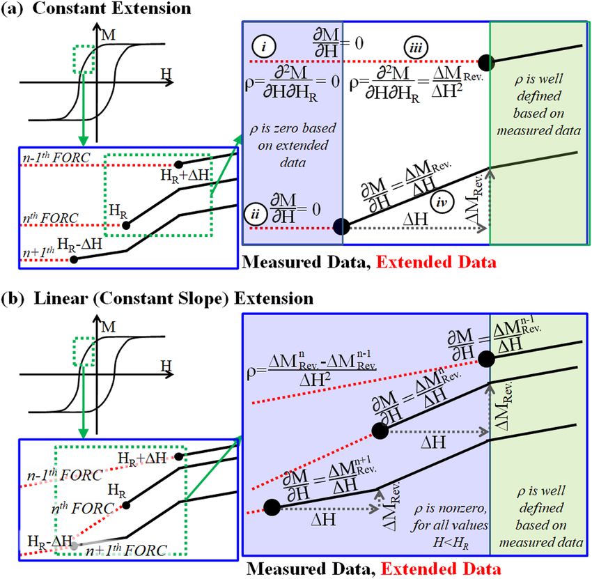
www.nature.com/scientificreports/
(ii) Fe nanodots exhibiting both single domain and magnetic vortex configurations, and (iii) SmCo/Fe exchange
spring magnet films with applications in permanent magnets. In each case the major loop is reconstructed and
compared to the directly measured hysteresis loop; the loops are found to have excellent qualitative and even
statistical agreement, validating our approach. Then, using the FORC technique to uniquely identify magnetic
reversal behavior, phase separated hysteresis loops are reconstructed. This technique allows for the extraction of
magnetometry metrics for individual phases within a multi-phase material, which is often difficult, even impos-
sible, when considering major loops alone.
Experiment
In order to highlight the versatility of the FORC technique, three distinctly different types of systems are con-
sidered. The first example is a high magnetic anisotropy FePt based system, where a common challenge is the
quantification of the A1 to L10 phase transformation. Here the L10/A1 mixed-phase F e39Cu16Pt45 thin films were
deposited at room-temperature using an atomic multilayer sputtering technique, and subsequently treated by
rapid thermal annealing (RTA), as reported p reviously42,43. For intermediate RTA temperatures at 300–400 °C,
the L10 and A1 phases are exchange coupled at the microscopic level. Measuring these samples with the applied
field in the out-of-plane (OOP) geometry, the A1 phase is reversibly forced OOP, while the (001) oriented L10
phase is hysteretic, thus representing an exchange coupled two-phase system with orthogonal easy axes. The
second example is arrays of Fe nanodots with average diameters of 52 nm, 58 nm, and 67 nm, respectively, with
edge-to-edge separation comparable to the dot diameter. They were grown by electron beam evaporation through
alumina shadow masks and a subsequent lift-off p rocess15,16,44. The smallest dots primarily undergo reversal by
highly coherent rotation, while the largest reverse primarily by a vortex nucleation/propagation/annihilation
mechanism. This transition occurs as a result of the geometrically dependent balance between the exchange
and magnetostatic energies. The medium sized dots (58 nm) show both reversal mechanisms due to a finite size
distribution, and represents a two-phase mixture system of weakly interacting elements. Lastly, the third example
is an exchange spring thin-film MgO/Cr(20 nm)/Sm2Co7(20 nm)/Fe(10 nm)/Cr(5 nm)—henceforth referred
to as SmCo/Fe—grown by magnetron s puttering12. As the applied magnetic field is first reduced from positive
saturation to negative fields, the magnetically soft Fe film rotates reversibly with the field, while the magnetically
hard SmCo remains in its initial orientation. At a sufficiently large negative field, the magnetically hard SmCo
layer also switches; subsequently increasing the magnetic field, the ’winding’ of the Fe occurs in positive fields
due to its exchange coupling to the (now negatively saturated) S mCo6. This sample represents a two-phase system,
with strong exchange coupling between the phases across the interface.
FORC analysis. Magnetometry measurements for all samples were performed on a vibrating sample mag-
netometer (VSM) at room temperature. FORC measurements were performed following procedures outlined
previously8,10,35,45,46: From the positively saturated state the magnetic field is reduced to a scheduled reversal
field, HR, at which point the field sweep direction is reversed and the magnetization, M, is measured as the
applied field, H, is increased to positive saturation, defining a single FORC branch. This process is repeated for
HR between the positive and negative saturated states, thus capturing all reversible and irreversible behavior.
For a regular field step of ∆H, the n + 1th FORC branch will begin at HRn+1 = HRn − H . A mixed second order
derivative is applied to the dataset to extract the normalized FORC distribution:
1 ∂ ∂M(H, HR )
ρ(H, HR ) = − (1)
2MS ∂HR ∂H
Following the measurement sequence provided above, as H is increased from an HR towards positive satura-
tion, the FORC branch probes the up-switching field for all the magnetic elements that have been down-switched
at HR ; up-switching events along this particular FORC are identified explicitly by the derivative dM/dH. Sub-
sequently, by taking the dHR derivative, the new up-switching events on each FORC branch are isolated46. New
up-switching events on the FORC branch starting at HRn are not present on the branch starting at HRn−1, illus-
trating that the HR-axis probes down-switching events. Thus the H and HR axes separately identify the up- and
down-switching events, but not necessarily of the same magnetic element; the FORC technique has no spatial
resolution and cannot attribute up- and down-switching events to any particular element. This distinction moti-
vates the term hysteron, which is used to illustrate an elemental hysteretic e vent35. However, correlating hysterons
to physical elements remains a challenge of the FORC t echnique23,46. The FORC diagrams can alternatively be
represented in terms of a local coercivity and bias field: HB = H+H 2 , HC =
R
2 .
H−HR
FORC projections are calculated by integrating the 2-dimensional FORC distribution over H or HR:
∞ ∞
f (HR ) = ρ(H, HR ) dH, and f (H) = ρ(H, HR )dHR (2)
−∞ −∞
Thus, for example, f (HR ) integrates all up-switching events that occur at each HR . Similarly, f (H) integrates
all down-switching events which would up-switch at each H . A subsequent integration of f (HR ) or f (H) over
all HR or H, respectively, would capture all switching events and recover the saturation magnetization—assum-
ing the reversible component is included in ρ34. In contrast, performing a partial integral, up to a dummy field
variable called HU , of the HR /H projection captures all the down/up switching events which have occurred up-to
HU . For example, �M(HR = Hu1 → ∞) = Hu1 −∞ ρ(H, HR ) dHdHR integrates the red region in Fig. 1, and
∞ ∞
recovers the magnetization of all elements which down-switch between HU1 < HR < ∞ (and up-switch between
−∞ < H < ∞). By then subtracting M from MS , the magnetization along the descending-field branch of the
Scientific Reports | (2021) 11:4018 | https://doi.org/10.1038/s41598-021-83349-z 2
Vol:.(1234567890)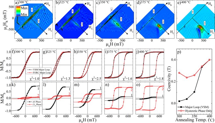
www.nature.com/scientificreports/
Figure 1. Schematic diagram illustrating the integration approach for recovering a major hysteresis loop from
the FORC diagram. The red-shaded region, integrated from the top of the panel down, recovers all of the down-
switching events between positive saturation and HU. The green-shaded region, integrated from left to right,
recovers all of the up-switching events from negative saturation to HU.
major loop at HU1 is recovered. Using a definite integral, e.g. spanning a defined parameter space, the magnetiza-
tion along the descending branch of the major loop can be calculated:
∞ ∞
M(HU1 ) = MS (1 − 2 ρ(H, HR )dHR dH) (3)
−∞ HU1
Similarly, integrating the H projection over −∞ < H < HU2, −∞ < HR < ∞, identified as the green region
in Fig. 1, calculates the magnetization of all of the up-switching events from negative saturation to HU2. Using
these values, the magnetization along the ascending branch of the major hysteresis loop can be determined:
HU2 ∞
M(HU2 ) = −M S (1 − 2 ρ(H, HR )dHR dH) (4)
−∞ −∞
Carrying out calculations of magnetization at varying HU1 (HU2 ) between the saturated states, according to
Eqs. (3) and (4), then recovers the descending and ascending-field branches of the major loop, respectively. The
leading factor of MS in Eqs. (3) and (4) cancels with the 1/MS prefactor in Eq. (1), resulting in an absolute scale;
for a normalized scale the prefactor in Eqs. (3) and (4) is one.
This integration technique becomes much more powerful when combined with FORC’s capability to resolve
multiple magnetic phases in a sample. That is, the FORC distribution has been demonstrated to uniquely identify
behaviors within multiphase systems. Here, we first discern the separate magnetic phases in the as-measured
FORC distribution and then employ Eqs. (3) and (4) to recover the phase-separated (major) hysteresis loops.
While the bounds of Eqs. (3) and (4) are infinite and H U1 and H U2—which can also span towards infinity—the
reconstruction of hysteresis loops from individual features must integrate over a truncated range that includes
only the FORC feature of interest. The bounds of this truncated space can be determined by the FORC distri-
bution merging with the background signal; integrating further recovers no additional contributions to the
magnetization since ρ = 0 in these regions.
Reversible features. Recovery of the embedded hysteresis loops often necessitates accurately accounting for the
reversible features. However, reversible features manifest on the H = HR boundary of the dataset, where the FORC
derivative is poorly defined. Specifically, the nth FORC branch has data spanning a field range HRn ≤ H ≤ HS ,
where HS is the saturation field, and the neighboring (n + 1)th FORC branch data spans HRn − H ≤ H ≤ HS .
Since there is no data
at M(H = HRn − H , HR = HRn), which is required to calculate the FORC distribution at
H = HR , HR = HRn , the derivative in Eq. (1) is now ill-defined. Due to this incomplete data set at the H = HR
n
boundary, reversible features—which by their very nature occur in this first field-step along a given FORC—are
often not reported in the literature, and focus is instead placed on the irreversible components away from the
H = HR boundary.
Previous work by Pike34 has demonstrated a constant extension scheme, graphically illustrated in Fig. 2a,
which recovers the reversible contribution to the magnetization. In this approach, the magnetization for H < HR
is defined as: M(H < HR ) ≡ M(HR ). Using this definition, ∂M ∂H H
www.nature.com/scientificreports/

                                            Figure 2.  Schematic diagram of (a) constant and (b) constant slope extensions applied to the family of FORCs.

                                            integration is performed. Below, we demonstrate that integrating the FORC distribution in (H, HR) coordinates
                                            can recover the major loop saturation magnetization, while integrating in the transformed (HB, HC) coordinates
                                            can suppress the reversible phase.
                                                A third approach most-often used to manage reversible behavior is to ‘clip’ the data-set. That is, to not cal-
                                            culate the FORC distribution in the region near the H = HR boundary of the dataset, until sufficient data at
                                            H ≥ HR are available to determine ρ. In so doing the reversible contribution is rejected and does not contribute
                                            to the weight of the resultant distribution. Furthermore, clipping the dataset has the consequence of removing
                                            features which may be hysteretic but with a small coercivity, especially when relatively large magnetic field step
                                            sizes are used in the measurement, and thus is less-than ideal for certain samples with a significant fraction of
                                            magnetically soft phases. These three approaches are demonstrated on each of the samples in the results section
                                            below and on a fully-reversible YIG sphere calibration standard in the supplemental material, Figure S1a-c.
                                                A physical picture based on Fig. 2 can be constructed and the integrated weight of the reversible FORC
                                            features calculated. The starting points on the n-1th, nth, and n + 1th FORC have coordinates (H, HR) of
                                            ( HRn + �H, HRn + �H), HRn , HRn , and HRn − �H, HRn − �H , respectively, marked by solid black dots.


                                               For the constant extension approach with ∂M(H
www.nature.com/scientificreports/
ible contributions on the nth FORC branch and manifests at H = H nR (i.e. HC = 0). Repeating this for all the FORC
branches and integrating the FORC distribution:
∞ ∞ ∞ ∞ ∞ HR +�H ∞ HR
ρ dHdHR = ρ dHdHR + ρ dHdHR + ρ dHdHR
−∞ −∞ −∞ HR +�H −∞ HR −∞ −∞
�M n Major Loop
Rev
= MSIrr + �H 2 + 0 = MSIrr + MSRev = MS
n
�H 2
(6)
where the integral was re-written to reflect the discrete stepping performed in the FORC measurement. These
integrals represent the region H > HR, H = HR and H < HR, respectively, e.g. the traditional FORC measurement,
the reversible region, and the extended region which contributes zero. Thus, the analytical calculation shows
integrating the constant extension accurately recovers the full saturation magnetization. This exercise also pro-
vides another useful insight: the constant extension to the dataset does not contribute to the FORC distribution
except at the boundary.
Similar calculations can be performed on the linear extended data. Using Fig. 2b and Eq. (1), the weight of the
FORC distribution at any point in the extended region, including the boundary of the dataset, can be calculated:
n n−1
1 �MREV �MREV
ρ≈ �H ( �H − �H ). Then, integrating the FORC distribution in (H, HR ) coordinates:
∞ ∞ ∞ ∞ ∞ HR
(�M n n−1
n
2 HR − H q
REV− �MREV )
ρ dHdHR = ρ dHdHR + ρ dHdHR = MSIrr + �H
−∞ Hq −∞ HR −∞ Hq n
�H 2 �H
(7)
where Hq is a dummy variable more negative than the negative saturation field (Hq < −HS ) defining the bound-
ary of the integration space. Next, noting that neighboring FORC branches are separated in HR by H in a regular
FORC dataset, this can be expanded by applying the same discrete stepping discussed above:
∞ ∞
1
0
ρ dHdHR = MSIrr. + 1 0
( HR − Hq �MREV − �MREV
−∞ Hq �H
(8)
+ HR0 − �H − Hq �MREV 2 1
− �MREV
0
3 2
+ HR − 2�H − Hq �MREV − �MREV + ...
Sat−1
1
= MSIrr. + n HSat
+ HRSat − Hq MREV 0
− HR0 − Hq MREV = MSIrr. + MSRev.
H MREV
H
n=1
where we have used the superscript to identify the FORC branch, with 0 and HSat identifying branches start-
ing from the positively saturated state, and achieving negative saturation, e.g. at HR = HSat. We also use the fact
that, at saturation there is no reversible contribution, and thus MREV
HSat = M 0
REV = 0. Indeed, integrating the
linear extended data in H/HR coordinates recovers the total saturation magnetization, with both the reversible
and irreversible contributions. We also note that the variable Hq drops out in the final solution; Hq can thus be
extended to negative saturation, integrating the entire parameter space without additional contributions to the
integrated magnetization.
Lastly, integrating the linear extended FORC distribution in the (HC, HB) parameter space:
√
∞ ∞ ∞ ∞ ∞ 0
(�M n − �M n−1 ) 2Hq
REV REV
ρ dHC dHB = ρ dHC dHB + ρdHC dHB = MSIrr. + �H 2
−∞ −∞ −∞ 0 −∞ Hq n
�H 2 �H
√
2Hq
= MSIrr. + 1 0 2 1 3 2
( �MREV − �MREV + �MREV − �MREV + �MREV − �MREV + ...)
�H
√
2Hq
= MSIrr. + HSat 0
= MSIrr.
�MREV − �MREV
�H
(9)
As noted above, MREV HSat = M 0
REV = 0 presuming the first and last FORC branches start and end in a
saturated state, and there is no Hq in the final result; integrating the linear extended FORC distribution in ( HC,
HB) coordinate system recovers only the irreversible component of the magnetization. This can be qualitatively
visualized in the supplemental Figure S1d and can be conceptually understood as integrating the FORC feature
with axes parallel to the reversible feature versus at 45°. This approach thus allows the irreversible features to be
quantitatively separated without arbitrary clipping of the data, allowing powerful new insights to be made into
mixed phase systems.
Results
Reversible feature. FORC distributions for the FeCuPt annealed at 350 °C (Fig. 3a–c), 67 nm diameter
Fe dots (Fig. 3d–f), and the Fe/SmCo exchange spring samples (Fig. 3g–i) were processed using clipping (top
row), constant (middle row) and linear (bottom row) extensions. As discussed above, the clipped data entirely
removes the reversible feature, while the constant extension method reveals a reversible feature only at H = HR .
Integrating the clipped data recovers an approximate ratio for the irreversible magnetization vs. major loop
Scientific Reports | (2021) 11:4018 | https://doi.org/10.1038/s41598-021-83349-z 5
Vol.:(0123456789)
www.nature.com/scientificreports/
MajorLoop
saturation magnetization MSIrr /MS of (3a) 0.28, (3d) 0.53, and (3g) 0.67. By comparison, integrating
the constant extension distributions (middle row of Fig. 3) accurately recovers the major loop saturation, with
MajorLoop
MSFORC /MS of (3b) 1.03, (3e) 0.98, and (3h) 0.94.
Comparing the above values from the clipped and constant extension data confirms the above derivations;
similar analysis confirms the constant-slope extension. Integrating the FORC distribution with a constant-slope
MajorLoop
extension in (HC , HB ) recovers a magnetization of MSFORC /MS =(3c) 0.35, (3f) 0.53, and (3i) 0.55, in
reasonably good agreement with MSIrr. as measured by clipping. Integrating the FORC distribution processed with
a constant-slope extension in (H, HR ) coordinates accurately recovers the major loop saturation magnetization:
MajorLoop
MSFORC /MS =(3a) 0.9, (3b) 1.0, (3c) 0.9. Thus, we confirm good agreement between the clipped dataset
and the linear extension in (HC , HB ) coordinates, as well as between the constant extension and the linear exten-
sion in (H, HR ) coordinates. It is less clear what additional information is recovered by integrating the linear
extended data (bottom row of Fig. 3).
A more definitive demonstration is shown in the FORC measurements of a YIG sphere (Supplemental Mate-
rials). The YIG sphere standard has a closed hysteresis loop, showing fully reversible behavior. Integrating the
FORC distribution processed with the different extensions recovers the major loop MS or zero.
In order to reconstruct the major loop the entire magnetization must be recovered and the constant extension
or linear extension (integrated in (H, HR )) must be utilized. However, when we consider applying the integrated
area represented by the red box in Fig. 1, to the constant-slope extension, shown in Fig. 3c,f,i, it is clear that the
integrated magnetization will depend on the integration limits in −H (analogous to the variable Hq discussed
above). For this reason, to reconstruct the major loop the constant extension is the reasonable choice.
Constructing hysteresis loops. Mixed phase FeCuPt. FeCuPt samples are annealed by RTA at 300–
400 °C, resulting in a mixed soft/hard A1/L10 phase. The FORC distributions, Fig. 4a–e, show the two-phase
system consisting of a mostly reversible A1 phase (located at HC = 0) and an irreversible L10 phase (located at
finite HC). Increasing the annealing temperature (left to right in Fig. 4) leads to a decrease in the weight of the
reversible phase, consistent with the transformation from the A1 to L10 phase. In the previous section the con-
stant extension was shown to recover the total saturation magnetization, as measured from the major loop, and
will be used here to reconstruct the major loop.
Performing the progressive integral of the FORC distribution along H and HR was suggested above to recover
the ascending and descending branches of the major loop (Eqs. 3 and 4), respectively. The reconstructed major
loops are shown superimposed with the major loops as measured directly with the VSM in Fig. 4f–j. The recon-
structed and directly measured major loops show excellent agreement. Quantitative agreement between the loops
is further shown by evaluating the difference between the loops and calculating the reduced χ2 comparing to a
null-set model (i.e. the model tests if the two loops are statistically identical). The error for each measurement
is defined by the machine sensitivity of 3 μemu. For every case the reduced χ2 is listed in the figure panel and is
approximately unity, confirming the excellent agreement within a characterized error.
Next, each of the two primary features in the FORC distribution are isolated and integrated to recover the
phase-separated hysteresis loops, Fig. 4k–o. Integrating the feature at (H = HR), labeled 1 in the FORC diagram,
recovers a major loop confirming its role as the reversible phase which diminishes with increased RTA tempera-
ture. The hysteretic phase, labeled 2 in the FORC diagrams, shows an open loop with increasing magnetization
and coercivity with increasing RTA temperature. Comparing these loops and the directly measured hysteresis
loops emphasizes the need to include the reversible feature in the above full-loop reconstruction. The coercivity
for the hysteretic phase is extracted and plotted in comparison to the major loop coercivity in Fig. 4p. At the
higher RTA temperatures, the hysteretic phase constitutes the majority of the sample and the coercivities agree
well. However, as the L10 phase fraction is reduced at lower RTA temperatures, coercivities from the major loop
and the extracted L10 phase diverge. The extracted L10 loop identifies that the coercivity of the L10 phase levels
off at approximately 250 mT at low annealing temperatures (red curve in Fig. 4p), even when the FeCuPt is
primarily in the A1 phase. This revelation provides sharp contrast to that from the measured major loop (black
curve in Fig. 4p), which shows HC roughly scales with annealing temperature. The reconstructed L10 loop thus
provides crucial insights to the ordering mechanism of the A1 to L10 phase transformation: this is consistent with
the nucleation/growth model of the L10 phase, which suggests that each grain should transform from A1 to the
high anisotropy L10 phase and is therefore expected to have a reasonable coercivity, once L10 ordering occurs.
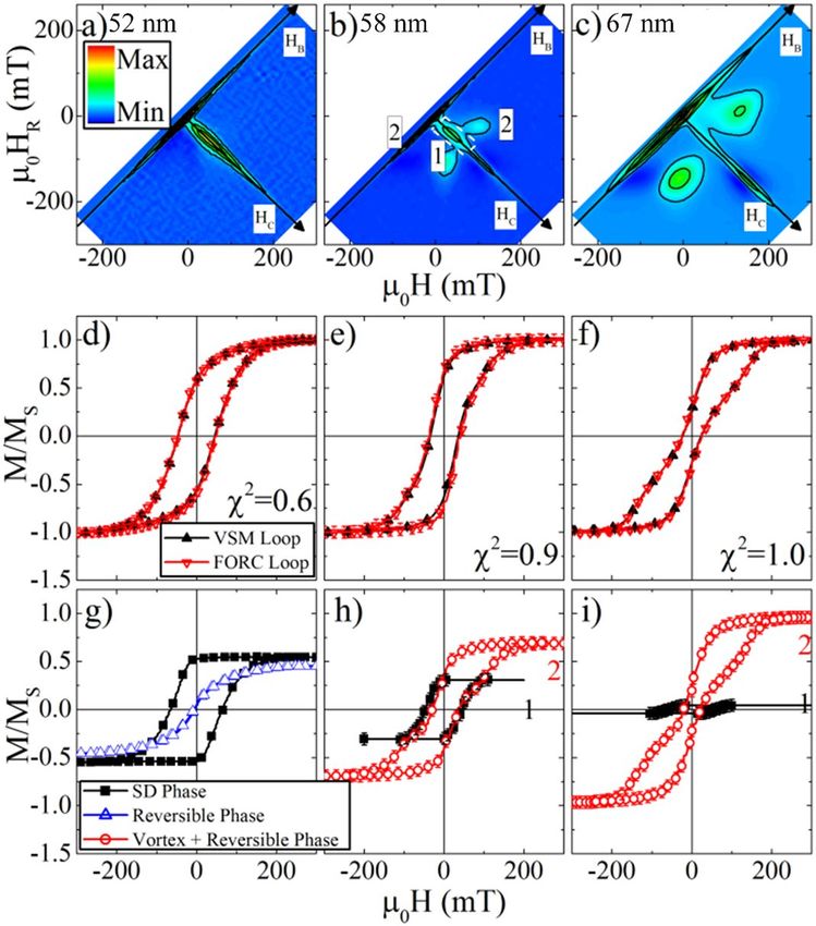
Single domain and vortex state Fe nanodots. FORC measurements of Fe nanodots, with average diameters of
52–67 nm, were one of the earliest applications for fingerprinting different reversal mechanisms and quantitative
phase fraction determination15,16. The FORC diagrams, Fig. 5a–c show the evolution from a single domain state,
52 nm diameter dots in panel (5a), to vortex-state reversal, 67 nm diameter dots in panel (5c). The intermedi-
ate sized dots, 58 nm diameter dots in panel (5b), show the presence of both reversal mechanisms. A reversible
feature is expected during vortex reversal, as the vortex core moves reversibly inside the nanodot in response to
an external magnetic field. Interestingly, all three samples show a significant feature at HC = 0 using the constant-
extension approach; the extent of the reversible feature along HB beyond the vortex annihilation feature and its
presence in the 52 nm sample indicates another reversible component. While this reversible component was not
addressed in the original study, some clues can be elucidated from the major loop, which clearly shows a reduced
remanence, MR/MS≈0.6. Note that these samples were prepared by evaporation through a self-assembled tem-
plate mask and exhibit a finite distribution of shapes and sizes15,16,44. This reversible component may represent
Scientific Reports | (2021) 11:4018 | https://doi.org/10.1038/s41598-021-83349-z 6
Vol:.(1234567890)www.nature.com/scientificreports/
Figure 3. FORC distributions of (a–c) FeCuPt annealed at 350 °C, (d–f) 67 nm Fe nanodots, and (g–i) Fe/
SmCo exchange-spring film.
a relaxation of the magnetization along the dot periphery preceding switching or perhaps even a distribution of
easy axes in the plane.
Similar to the FeCuPt samples, the major loops are reconstructed by progressively integrating the FORC
distribution, and compared to the VSM major loops in Fig. 5d–f. Again, the reconstructed major loops show
excellent qualitative and quantitative agreement with the directly measured major loops. Furthermore, using
the FORC diagram to separate the reversal mechanisms, the hysteresis loop for each phase is reconstructed in
Fig. 5g–i. For the 52 nm dots the single domain and reversible phases are plotted and, similar to the FeCuPt
sample, the coercivity for the hysteretic phase (66 mT) is significantly larger than the VSM major loop (46 mT).
From the saturation magnetization of each phase the reversible and hysteretic phases contribute similarly (45%
v. 55%) to the ensemble magnetism of the sample.
For the 58 nm and 67 nm dots, which possess three phases (single domain, vortex state, and reversible), only
the single domain phase can be separated, since the vortex-state and reversible contributions have overlapping
features at HC = 0. The single domain phase is shown to decrease in its contributions with increased dot size,
and possess a coercivity always much larger than the VSM major loop. The vortex + reversible phase, on the
other hand, develops into a wasp-waisted hysteresis loop and increases in weight with dot diameter, following
its increased vortex phase fraction.
Fe/SmCo exchange spring. The last example is a Fe/SmCo exchange spring thin-film shown in Fig. 6. As the
magnetic field is reduced from positive saturation to small negative fields, the SmCo remains positively saturated
while the Fe layer follows the field reversibly, which then relaxes to a positive orientation in the absence of a field
due to the exchange coupling to the SmCo. This reversible ’winding’ of the exchange spring occurs when the
applied field is anti-parallel to the SmCo layer and manifests as Feature 1 in Fig. 6a. Then, at sufficiently large
negative fields the SmCo reverses. Along the subsequent FORC branch, the reversible winding of the Fe layer
occurs now in positive fields—since the anchoring SmCo is now negatively oriented. Thus, along this FORC
branch there are three magnetic features: First, across the applied field range for the initial winding (Feature 1)
the magnetization versus field is now flat (SmCo and Fe are parallel and aligned with the magnetic field in the
negative direction), thus dM/dH over this range decreases, from a positive value to zero, with decreasing HR.
Following from Eq. (1), this generates a negative FORC feature (Feature 2); the origin of negative features was
discussed in previous works46. Continuing along this FORC branch, in positive magnetic fields the Fe reversibly
winds, with the SmCo still in the negative direction. This winding was absent on more-positive HR branches, and
so constitutes an increase in dM/dH with decreasing HR, generating a positive feature in the FORC distribution
(Feature 3). Finally, at large positive fields, the SmCo up-switches, generating Feature 4. The alignment in H of
Features 1 and 2 and alignment in HR of Features 2 and 3 attests to their common origin in the Fe layer.
The reconstructed major loop, shown in Fig. 6b, once again shows excellent qualitative and quantitative
agreement with the directly measured major loop. Phase separated major loops were calculated for each feature
labeled 1–4 in Fig. 6a, as shown in Fig. 6c. While the other FORC distributions had well-separated phases, for the
SmCo/Fe phases, Features 3 and 4 are all overlapping; the integrated weight of Feature 1 is used to set the limit
on the integration for Feature 3, thus separating the phases. Consistent with the explanation above, the loop from
Scientific Reports | (2021) 11:4018 | https://doi.org/10.1038/s41598-021-83349-z 7
Vol.:(0123456789)www.nature.com/scientificreports/
Figure 4. FORC distributions of (a–e) FeCuPt annealed at 300–400 °C, in 25 °C increments, (f–j) directly
measured (black, solid) and FORC reconstructed (red, open) major loop, and (k–o) phase separated major loops
for the A1 (black) and L10 (red) phase, respectively. The major loop and phase-separated coercivity trends are
collated in (p).
Feature 1 is closed, identifying the reversible winding of the Fe coming from positive saturation. Interestingly,
the loop for Feature 2, which comes from a negative FORC feature, results in an inverted hysteresis loop. The
descending branch of loop 2, e.g. from positive to negative magnetic fields, has a sharp switching event at the
SmCo switching field, then the ascending branch runs parallel to the Feature 1 loop. The inverted correlation
between the Feature 1 and 2 loops is a visual demonstration of the disappearance of the Fe winding in negative
fields after the SmCo reversal. The loop from Feature 2 also demonstrates that the FORC technique maps model
hysterons and not physical magnetic elements; the Feature 2 loop identifies the weight of the Fe layer, with an
up-switching of the SmCo reversal field, and a down-switching reflective of the Fe winding (coming from posi-
tive saturation). Similarly, the loop from Feature 3 shows a down-switching at the SmCo reversal field, and up-
switching as the Fe winds in positive fields, coming from negative saturation. Thus, between these three loops, all
of the behavior of the Fe is captured. The SmCo loop is also extracted, and gives values for the coercivity which
are consistent with the major loop value.
Conclusion
The FORC technique has become widely used in the magnetics community as a tool for identifying the micro-
scopic details of often complex systems through macroscopic measurements. A particular strength of the FORC
technique is its ability to uniquely identify and separate magnetic reversal behavior in multi-phase systems.
Within the magnetic “fingerprints” of each phase are details of the magnetization reversal which can be recov-
ered through appropriate numerical treatment. Prerequisite to this treatment was proper consideration of the
reversible phase. Constant and linear data extensions were analytically and empirically demonstrated. Using a
constant data extension, the major hysteresis loop was reconstructed from the FORC distribution. Then, using
the FORC technique to uniquely identify magnetization reversal behaviors, phase separated hysteresis loops
were reconstructed. These phase-resolved loops contained the traditional metrics of magnetic reversal behavior,
including the coercivity and saturation field, and the remanent and saturation magnetization (which can be
correlated to phase fraction). This work addresses traditional issues extant with the FORC technique—namely
reversible features—and also promotes a new approach, which builds a bridge between the FORC technique
and traditional magnetometry.
Scientific Reports | (2021) 11:4018 | https://doi.org/10.1038/s41598-021-83349-z 8
Vol:.(1234567890)www.nature.com/scientificreports/
Figure 5. FORC distributions of (a–c) 52 nm, 58 nm, and 67 nm diameter Fe nanodots, (d–f) directly
measured (black, solid) and FORC reconstructed (red, open) major loop, and (g–i) phase separated major
loops, respectively. The single-domain and vortex features are identified in (b) by 1 and 2, respectively. The area
selected for reconstructing the single-domain loop for the 58 nm dots is shown as the dashed white box in (b).
Figure 6. FORC distribution of (a) Fe/SmCo exchange-spring film, (b) directly measured (black, solid) and
FORC reconstructed (red, open) major loop, and (c) phase separated loops identified with features 1–4, labeled
in panel (a).
Received: 20 November 2020; Accepted: 11 January 2021
References
1. Wu, J. & Leighton, C. Glassy ferromagnetism and magnetic phase separation in La1-xSrxCoO3. Phys. Rev. B 67, 174408. https://doi.
org/10.1103/PhysRevB.67.174408 (2003).
2. Kryder, M. H. et al. Heat assisted magnetic recording. Proc. IEEE 96, 1810–1835. https://doi.org/10.1109/JPROC.2008.2004315
(2008).
10 FePtX–Y media for heat-assisted magnetic recording. Phys. Status
3. Weller, D., Mosendz, O., Parker, G., Pisana, S. & Santos, T. S. L
Solidi A 210, 1245–1260. https://doi.org/10.1002/pssa.201329106 (2013).
4. Bader, S. D. Colloquium: Opportunities in nanomagnetism. Rev. Mod. Phys. 78, 1. https://doi.org/10.1103/RevModPhys.78.1
(2006).
5. Cowburn, R., Koltsov, D., Adeyeye, A., Welland, M. & Tricker, D. Single-domain circular nanomagnets. Phys. Rev. Lett. 83,
1042–1045. https://doi.org/10.1103/PhysRevLett.83.1042 (1999).
Scientific Reports | (2021) 11:4018 | https://doi.org/10.1038/s41598-021-83349-z 9
Vol.:(0123456789)www.nature.com/scientificreports/
6. Fullerton, E. E., Jiang, J. S., Grimsditch, M., Sowers, C. H. & Bader, S. D. Exchange-spring behavior in epitaxial hard/soft magnetic
bilayers. Phys. Rev. B 58, 12193. https://doi.org/10.1103/PhysRevB.58.12193 (1998).
7. Zeng, H., Li, J., Liu, J. P., Wang, Z. L. & Sun, S. H. Exchange-coupled nanocomposite magnets by nanoparticle self-assembly. Nature
420, 395–398. https://doi.org/10.1038/nature01208 (2002).
8. Pike, C. R., Roberts, A. P. & Verosub, K. L. Characterizing interactions in fine magnetic particle systems using first order reversal
curves. J. Appl. Phys. 85, 6660. https://doi.org/10.1063/1.370176 (1999).
9. Katzgraber, H. G. et al. Reversal-field memory in the hysteresis of spin glasses. Phys. Rev. Lett. 89, 257202. https://doi.org/10.1103/
PhysRevLett.89.257202 (2002).
10. Davies, J. E. et al. Magnetization reversal of Co/Pt multilayers: Microscopic origin of high-field magnetic irreversibility. Phys. Rev.
B 70, 224434. https://doi.org/10.1103/PhysRevB.70.224434 (2004).
11. Spinu, L., Stancu, A., Radu, C., Feng, L. & Wiley, J. B. Method for magnetic characterization of nanowire structures. IEEE Trans.
Magn. 40, 2116–2118. https://doi.org/10.1109/tmag.2004.829810 (2004).
12. Davies, J. E. et al. Anisotropy-dependence of irreversible switching in Fe/SmCo and FeNi/FePt spring magnet films. Appl. Phys.
Lett. 86, 262503. https://doi.org/10.1063/1.1954898g (2005).
13. Davies, J. E., Wu, J., Leighton, C. & Liu, K. Magnetization reversal and nanoscopic magnetic phase separation in L a1-xSrxCoO3.
Phys. Rev. B 72, 134419. https://doi.org/10.1103/PhysRevB.72.134419 (2005).
14. Beron, F. et al. First-order reversal curves diagrams of ferromagnetic soft nanowire arrays. IEEE Trans. Magn. 42, 3060–3062. https
://doi.org/10.1109/TMAG.2006.880147 (2006).
15. Dumas, R. K., Li, C. P., Roshchin, I. V., Schuller, I. K. & Liu, K. Magnetic fingerprints of sub-100 nm Fe dots. Phys. Rev. B 75,
134405. https://doi.org/10.1103/PhysRevB.75.134405 (2007).
16. Dumas, R. K., Liu, K., Li, C. P., Roshchin, I. V. & Schuller, I. K. Temperature induced single domain-vortex state transition in sub-
100 nm Fe nanodots. Appl. Phys. Lett. 91, 202501. https://doi.org/10.1063/1.2807276 (2007).
17. Chiriac, H., Lupu, N., Stoleriu, L., Postolache, P. & Stancu, A. Experimental and micromagnetic first-order reversal curves analysis
in NdFeB-based bulk “exchange spring”-type permanent magnets. J. Magn. Magn. Mater. 316, 177–180. https://doi.org/10.1016/j.
jmmm.2007.02.049 (2007).
18. Rahman, M. T. et al. Controlling magnetization reversal in Co/Pt nanostructures with perpendicular anisotropy. Appl. Phys. Lett.
94, 042507. https://doi.org/10.1063/1.3075061 (2009).
19. Rotaru, A. et al. Interactions and reversal-field memory in complex magnetic nanowire arrays. Phys. Rev B. 84, 134431. https://
doi.org/10.1103/PhysRevB.84.134431 (2011).
20. Kou, X. et al. Memory effect in magnetic nanowire arrays. Adv. Mater. 23, 1393. https://doi.org/10.1002/adma.201003749 (2011).
21. Navas, D. et al. Magnetization reversal and exchange bias effects in hard/soft ferromagnetic bilayers with orthogonal anisotropies.
New J. Phys. 14, 113001. https://doi.org/10.1088/1367-2630/14/11/113001 (2012).
22. Fang, Y. et al. A nonvolatile spintronic memory element with a continuum of resistance states. Adv. Funct. Mater. 23, 1919–1922.
https://doi.org/10.1002/adfm.201202319 (2013).
23. Dobrota, C.-I. & Stancu, A. What does a first-order reversal curve diagram really mean? A study case: Array of ferromagnetic
nanowires. J. Appl. Phys. 113, 043928. https://doi.org/10.1063/1.4789613 (2013).
24. Chen, A. P. et al. Magnetic properties of uncultivated magnetotactic bacteria and their contribution to a stratified estuary iron
cycle. Nat. Commun. 5, 4797. https://doi.org/10.1038/ncomms5797 (2014).
25. Gilbert, D. A. et al. Realization of ground state artificial skyrmion lattices at room temperature. Nat. Commun. 6, 8462. https://
doi.org/10.1038/ncomms9462 (2015).
26. Gilbert, D. A. et al. Structural and magnetic depth profiles of magneto-ionic heterostructures beyond the interface limit. Nat.
Commun. 7, 12264. https://doi.org/10.1038/ncomms12264 (2016).
27. Zamani Kouhpanji, M. R., Ghoreyshi, A., Visscher, P. B. & Stadler, B. J. H. Facile decoding of quantitative signatures from magnetic
nanowire arrays. Sci. Rep. 10, 15482. https://doi.org/10.1038/s41598-020-72094-4 (2020).
28. Ramirez, J. G., Sharoni, A., Dubi, Y., Gomez, M. E. & Schuller, I. K. First-order reversal curve measurements of the metal-insulator
transition in VO2: Signatures of persistent metallic domains. Phys. Rev. B 79, 235110. https://doi.org/10.1103/PhysRevB.79.23511
0 (2009).
29. Gilbert, D. A. et al. Tunable low density palladium nanowire foams. Chem. Mater. 29, 9814–9818. https://doi.org/10.1021/acs.
chemmater.7b03978 (2017).
30. Frampton, M. K. et al. First-order reversal curve of the magnetostructural phase transition in FeTe. Phys. Rev. B 95, 214402. https
://doi.org/10.1103/PhysRevB.95.214402 (2017).
31. Roberts, A. P., Pike, C. R. & Verosub, K. L. First-order reversal curve diagrams: A new tool for characterizing the magnetic proper-
ties of natural samples. J. Geophys. Res. 105, 28461–28475. https://doi.org/10.1029/2000JB900326 (2000).
32. Valcu, B. F., Gilbert, D. A. & Liu, K. fingerprinting inhomogeneities in recording media using the first order reversal curve method.
IEEE Trans. Magn. 47, 2988. https://doi.org/10.1109/TMAG.2011.2146241 (2011).
33. Gilbert, D. A. et al. Magnetic yoking and tunable interactions in FePt-based hard/soft bilayers. Sci. Rep. 6, 32842. https://doi.
org/10.1038/srep32842 (2016).
34. Pike, C. R. First-order reversal-curve diagrams and reversible magnetization. Phys. Rev. B 68, 104424. https://doi.org/10.1103/
PhysRevB.68.104424 (2003).
35. Pike, C. R., Ross, C. A., Scalettar, R. T. & Zimanyi, G. T. First-order reversal curve diagram analysis of a perpendicular nickel
nanopillar array. Phys. Rev. B 71, 134407. https://doi.org/10.1103/PhysRevB.71.134407 (2005).
36. Stancu, A., Ricinschi, D., Mitoseriu, L., Postolache, P. & Okuyama, M. First-order reversal curves diagrams for the characterization
of ferroelectric switching. Appl. Phys. Lett. 83, 3767–3769. https://doi.org/10.1063/1.1623937 (2003).
37. Samanifar, S., Kashi, M. A. & Ramazani, A. Study of reversible magnetization in FeCoNi alloy nanowires with different diameters
by first order reversal curve (FORC) diagrams. Phys. C 548, 72–74. https://doi.org/10.1016/j.physc.2018.02.009 (2018).
38. Bodale, I., Stoleriu, L. & Stancu, A. Reversible and irreversible components evaluation in hysteretic processes using first and
second-order magnetization curves. IEEE Trans. Magn. 47, 192–197. https://doi.org/10.1109/TMAG.2010.2083679 (2011).
39. Harrison, R. J. & Feinberg, J. M. FORCinel: An improved algorithm for calculating first-order reversal curve distributions using
locally weighted regression smoothing. Geochem. Geophys. Geosyst. 9, Q05016. https://doi.org/10.1029/2008GC001987 (2008).
40. Burks, E. C. et al. 3D Nanomagnetism in low density interconnected nanowire networks. Nano Lett. 21, 716-722. https://doi.
org/10.1021/acs.nanolett.0c04366 (2021).
41. Lascu, I. et al. Magnetic unmixing of first-order reversal curve diagrams using principal component analysis. Geochem. Geophys.
Geosyst. 16, 2900–2915. https://doi.org/10.1002/2015GC005909 (2015).
42. Gilbert, D. A. et al. Probing the A1 to L 10 transformation in FeCuPt using the first order reversal curve method. APL Mater. 2,
086106. https://doi.org/10.1063/1.4894197 (2014).
43. Gilbert, D. A. et al. Tuning magnetic anisotropy in (001) oriented L 10 (Fe1-xCux)55Pt45 films. Appl. Phys. Lett. 102, 132406. https://
doi.org/10.1063/1.4799651 (2013).
44. Liu, K. et al. Fabrication and thermal stability of arrays of Fe nanodots. Appl. Phys. Lett. 81, 4434–4436. https://doi.
org/10.1063/1.1526458 (2002).
45. Mayergoyz, I. D. Mathematical Models of Hysteresis (Springer, Berlin, 1991).
Scientific Reports | (2021) 11:4018 | https://doi.org/10.1038/s41598-021-83349-z 10
Vol:.(1234567890)www.nature.com/scientificreports/
46. Gilbert, D. A. et al. Quantitative decoding of interactions in tunable nanomagnet arrays using first order reversal curves. Sci. Rep.
4, 4204. https://doi.org/10.1038/srep04204 (2014).
Acknowledgements
This work has been supported by the NSF (ECCS-1611424 and ECCS-1933527) and DOE Career
(DE-SC0021344).
Author contributions
R.K.D., J.D., J.R., P.M. and D.A.G. performed the measurements. J.R., P.M. and D.A.G. processed the experimental
data and established the underlying mechanics. D.A.G. and K.L. designed the experiments. D.A.G. and K.L. wrote
the initial drafts of the manuscript and all authors contributed to its review and editing.
Competing interests
The authors declare no competing interests.
Additional information
Supplementary Information The online version contains supplementary material available at https://doi.
org/10.1038/s41598-021-83349-z.
Correspondence and requests for materials should be addressed to D.A.G.
Reprints and permissions information is available at www.nature.com/reprints.
Publisher’s note Springer Nature remains neutral with regard to jurisdictional claims in published maps and
institutional affiliations.
Open Access This article is licensed under a Creative Commons Attribution 4.0 International
License, which permits use, sharing, adaptation, distribution and reproduction in any medium or
format, as long as you give appropriate credit to the original author(s) and the source, provide a link to the
Creative Commons licence, and indicate if changes were made. The images or other third party material in this
article are included in the article’s Creative Commons licence, unless indicated otherwise in a credit line to the
material. If material is not included in the article’s Creative Commons licence and your intended use is not
permitted by statutory regulation or exceeds the permitted use, you will need to obtain permission directly from
the copyright holder. To view a copy of this licence, visit http://creativecommons.org/licenses/by/4.0/.
© The Author(s) 2021
Scientific Reports | (2021) 11:4018 | https://doi.org/10.1038/s41598-021-83349-z 11
Vol.:(0123456789)You can also read