Reversal of Fortune for Political Incumbents Evidence from Oil Shocks - World Bank Documents
←
→
Page content transcription
If your browser does not render page correctly, please read the page content below
Public Disclosure Authorized

                               Policy Research Working Paper                    9287
Public Disclosure Authorized

                                 Reversal of Fortune for Political Incumbents

                                                Evidence from Oil Shocks
                                                                Rabah Arezki
Public Disclosure Authorized

                                                               Simeon Djankov
                                                                 Ha Nguyen
                                                                 Ivan Yotzov
Public Disclosure Authorized

                               Middle East and North Africa Region
                               Office of the Chief Economist
                               June 2020
Policy Research Working Paper 9287
Abstract
Using a new dataset of 207 national elections across 50 oil price increases systematically lower the odds of reelection
democracies, this paper is the first to systematically exam- for incumbents and increase the likelihood of changes in
ine the effects of oil price shocks on incumbents’ political the ideology of the incoming government. These shocks are
fortunes in developed oil-importing countries. We find that found to operate through lowering consumption growth.
This paper is a product of the Office of the Chief Economist, Middle East and North Africa Region. It is part of a larger
effort by the World Bank to provide open access to its research and make a contribution to development policy discussions
around the world. Policy Research Working Papers are also posted on the Web at http://www.worldbank.org/prwp. The
authors may be contacted at rarezki@worldbank.org.
The Policy Research Working Paper Series disseminates the findings of work in progress to encourage the exchange of ideas about development
issues. An objective of the series is to get the findings out quickly, even if the presentations are less than fully polished. The papers carry the
names of the authors and should be cited accordingly. The findings, interpretations, and conclusions expressed in this paper are entirely those
of the authors. They do not necessarily represent the views of the International Bank for Reconstruction and Development/World Bank and
its affiliated organizations, or those of the Executive Directors of the World Bank or the governments they represent.
Produced by the Research Support TeamReversal of Fortune for Political Incumbents:
Evidence from Oil Shocks ∗
Rabah Arezki, Simeon Djankov, Ha Nguyen, Ivan Yotzov
Originally published in the Policy Research Working Paper Series on June, 2020. This version
is updated on March, 2021.
To obtain the originally published version, please email prwp@worldbank.org.
Keywords: Elections, Incumbent, Oil Prices, Economic Shocks.
JEL Codes: D72; E21; P16; Q43.
∗ Rabah Arezki is the Chief Economist of the African Development Bank and a Senior Fellow at
Harvard’s Kennedy School of Government. Simeon Djankov is Director for Policy with the Financial
Markets Group at the London School of Economics and Senior Fellow at the Peterson Institute for
International Economics. Ha Nguyen is a Senior Economist in the Chief Economist Office of the Middle
East and North Africa at the World Bank. Ivan Yotzov is PhD candidate at the University of Warwick.
We thank Jeremy Evans and Nick Lore-Edwards for comments. The findings, interpretations, and
conclusions expressed in this paper do not necessarily reflect the views of the World Bank, the African
Development Bank, or the governments they represent. The World Bank and the African Development
Bank do not guarantee the accuracy of the data included in this work.1 Introduction
The increase in gasoline prices stemming from the oil crisis overshadowed the
United States presidential debate of October 1980. Ronald Reagan and then-President
Jimmy Carter were going head to head in the election. Carter’s loss that year coin-
cided with a peak in oil prices. Other modern US presidential incumbents – for
example, Presidents Ford and George H.W. Bush - also lost their reelection bids fol-
lowing oil price spikes. This anecdotal evidence points to a broader question about
the role of exogenous shocks in determining electoral outcomes.
Our paper is the first effort to systematically examine the effect of oil price shocks
on the reelection probability of political incumbents in oil-importing countries. We
use a novel dataset of 207 national elections in 50 mostly oil-importing democracies,
which crucially also includes polling data in the run-up to elections. The polling data
allow us to explore the effect of exogenous shocks not only on the election outcome,
but also on voting intentions in the months leading up to the vote. Depending on the
political system, the dataset includes elections of the chief executive in parliamentary
or presidential systems. As large oil imports leave a country vulnerable to changes
in international crude oil prices, we rely on these prices as an exogenous source of
country-specific variation in terms of trade. Specifically, we create a measure of ’oil
price shock’ by interacting the fluctuations in international oil prices (over which
individual countries do not have explicit control) with the country-specific intensity
of oil imports relative to GDP.
An oil price shock one year prior to an election is found to significantly reduce
the likelihood of reelection for the incumbent party. Specifically, a 1% increase in
our oil shock measure decreases the likelihood of incumbent re-election by nearly six
percentage points. Furthermore, novel polling data confirm that these shocks operate
by reducing the popularity of the sitting government. We show that both right-wing
and left-wing incumbent parties are susceptible to crude oil price increases. We verify
that the winning parties are more likely to belong to the opposite end of the political
spectrum. In other words, following an oil price increase, a left-leaning incumbent
party is more likely to be replaced by a right-leaning party and vice versa.
Since most countries in our sample are oil importers, an increase in crude oil
prices would reduce the purchasing power of the population, consistent with Hamil-
ton (2003) and Blanchard and Gali (2009). Consistent with this logic, we show that
an increase in oil prices is found to reduce consumption growth. This is a potential
2mechanism which links oil price movements with voter behavior in elections. Inter-
estingly, oil shocks do not impact output growth significantly, as one would typically
expect.
The results remain robust to a variety of checks and alternative specifications.
When we use changes in import commodity prices for 45 commodities instead of oil
prices only, we find that an increase in the import prices one year prior to elections
is significantly associated with a reduction in the odds of incumbent reelection. Our
results also survive when we control for voter turnout, pre-determined elections,
other macro variables, and different lags for oil shocks.
This paper is related to several strands of the literature. First, it contributes to the
literature on retrospective voting, which highlights cases in which incumbent gov-
ernments are punished for events out of their control1 . Many studies discuss the
effects of natural disasters on local elections (see, for example, Gasper and Reeves,
2011; Healy and Malhotra, 2010; Cole et al., 2012; Wang and Berdiev, 2015; Achen and
Bartels, 2017). A consistent finding from these studies is that incumbents’ electoral
fortunes suffer after natural disasters. The finding is intuitive as the impacts of nat-
ural disasters are generally dramatic and concentrated at the local level. In contrast,
we show that relatively more subtle events, such as oil price fluctuations, can also be
powerful factors influencing political outcomes.
Our paper is related to a rich literature on the political effects of commodity booms
and busts in commodity exporters that operate via commodity price windfalls2 .
These studies can roughly be divided into those studying the effects of commod-
ity price shocks on conflict versus those on elections or democratic transitions. The
formers find a nuanced relationship between resource wealth and conflict, depend-
ing on the region, time period, and precise commodities considered3 . The studies of
commodity price shocks and democratic transitions also provide mixed conclusions4 .
Our paper is related but distinct from this literature. It examines the impact of oil
price shocks on incumbent’s political fortune in a set of predominantly developed
oil-importing countries. The impact is found to operate via changes in consumption
growth.
Finally, our paper is related to the political business cycle literature that examines
1 See Healy and Malhotra (2013) for a review of the retrospective voting literature.
2 See van der Ploeg (2011) for a excellent survey.
3 See Bruckner and Ciccone (2010), Bazzi and Blattman (2014), Dube and Vargas (2013).
4 See Bruckner et al. (2012), Caselli and Tesei (2016), Andersen and Aslaksen (2013), Burke and
Leigh (2010).
3how political cycles could affect economic outcomes. The literature tends to find weak
effects in developed countries, with the US being a notable exception (see Alesina and
Rosenthal, 1995 and Alesina et al., 1997). The effects are stronger in more immature
democracies. For example, Russia’s regional public expenditure rises shortly before
regional elections (Akhmedov and Zhuravskaya, 2004). This lends support to the
argument that the strengths of a democracy – such as press freedom, checks and bal-
ances, or accountability – can help mitigate opportunistic political cycles (Akhmedov
and Zhuravskaya, 2004 and Aidt et al., 2011).
The remainder of the paper is as follows. Section 2 presents the data. Section
3 shows the main results. Section 4 presents several robustness checks. Section 5
concludes.
2 Data
Our analysis draws on two main datasets. The first covers election polls and
outcomes for 207 elections across 50 countries worldwide over the period 1980-2020.
Only elections with available polling data are included. On average, each country
has four elections. There are 149 parliamentary and 58 presidential elections. The
list of countries and the number of elections in each country by year are presented
in Figure 1 and Table A1. The polling data originate from multiple polling agencies
for each country. Official election results are available from multiple sources. For
each election, voting intentions by political party (i.e. polls) are gathered, alongside
election outcomes5 . It is important to consider the incumbent changes at the political
party level rather than for individual politicians, since term limits could create me-
chanical turnover of individuals. Countries for which polling data are unavailable are
not included in our dataset. In total, the dataset has over 13,333 polling observations,
which are aggregated into 2,552 election-month polling observations for the incum-
bent party. Hence, on average, each election has about 12 election-month polling
observations.
In addition to voter intentions, we include data on several additional election
characteristics. First, an indicator variable is created to denote elections where the
incumbent party remains in power following the election. This variable is at the party-
5 In
some polls, respondents are allowed to answer election questions with “Don’t Know” or “Not
Sure”. This will mechanically make voting intentions incompatible with the final election outcomes.
In such cases, we drop the extraneous responses, and rescale the polls, considering only respondents
who have selected a political party.
4level, and therefore term limits will not affect the outcome. For example, consider the
1988 US Presidential Election. George H.W. Bush was elected president, after Ronald
Reagan served two terms. Since the Republican party remained in power, we treat
that episode as the incumbent staying in power.
In cases of political coalitions, where multiple parties form the government, our
measure of incumbency considers the political party of the chief executive. Second,
we use data on the name of the political party incumbent, and the political party
which wins the election. With that data, the political orientation of the incumbents
and election winners are calculated based on party ideological orientation.
For the majority of elections and parties, data on left-right orientation are taken
from the ParlGov Party Database (Döring and Manow, 2019). This database contains
information for over 1,600 political parties in 37 democracies in the EU and OECD.
For each party, a time-invariant score between 0 and 10 is provided, classifying their
political position from left-wing to right-wing, respectively. This score, in turn, is
based on data from Castles and Mair (1984), Huber and Inglehart (1995), Benoit and
Laver (2006), and Bakker et al. (2015). For example, the UK Conservative Party has
a score of 7.4, while the French Socialist Party has a score of 3.2. In our analysis,
we do not use the continuous index, but rather split parties into left-wing and right-
wing using the threshold value of 5. Overall, this dataset provides information for
most countries in our sample. For countries outside the ParlGov sample (primarily
South America), we also classify incumbents and election winners as left-wing or
right-wing using various online sources. For example, Jair Bolsonaro, the winner
of the 2018 Brazilian general election is classified as right-wing, based on his then-
party, Partido Social Liberal. In sum, of the 207 elections in our main sample, there
are 91 left-wing incumbents and 116 right-wing incumbents. Separately, there are 82
left-wing election winners, and 125 right-wing election winners.
Finally, voter turnout data are collected, as well as an indicator for whether voting
is compulsory for a given election. Most of the data are from the IDEA Voter Turnout
Database; any gaps are supplemented using online sources.
The main source of shock is based on changes in international oil prices, weighted
by the average country-specific oil import values. International oil prices are obtained
from the World Bank “Pink Sheet” data. These data contain real and nominal crude
oil prices; for our main analysis, we use real oil prices. Data on the value of oil
imports and GDP in US dollars are obtained from the IMF’s World Economic Outlook.
5The country-year weights are constructed by taking three-year rolling averages of oil
imports to GDP. Combining these weights with oil prices, our main index for country
i and year t is constructed as:
∆ ln(Crude Oil Index )i,t = ∆[ln(Crude Oil Price)t × Ωi,Oil,t ]
The weights, Ωi,Oil,t ,are calculated as:
1 Oil Import Oil Import Oil Import
Ωi,Oil,t = + +
3 GDP t −1 GDP t −2 GDP t −3
Although the main results in this paper are based on oil shocks constructed with real
oil prices and three-year rolling average weights, all results are also robust to the use
of nominal prices, and five-year rolling weights.
The next data source is the Commodity Terms of Trade Database introduced in
Gruss and Kebhaj (2019). These data consist of country-specific commodity price
indices, based on a set of 45 individual commodities. The formula for the gross
import price index is:
J
∆ ln( Import ComPI )i,t = ∑ ∆Pj,t Ωi,j,t
j =1
In the above specification, Pj,t refers to the logarithm of the real price of commodity
j in time period t. Ωi,j,t denote the commodity-country-specific weights by which
the prices are weighted. The country specific weights are based on the ratio of gross
imports to GDP. Rolling weights use a moving average of the last three time periods
before t to construct Ωi,j,t . The commodity price indices are available at both an
annual and monthly frequency over our sample period. We use the annual data for
our main specification and turn to monthly data when considering the polling data.
We show that our results are robust to using rolling as well as fixed weights.
Table 1 provides summary statistics for the key variables. The average oil shock
in election years in real terms is -0.16%, and 0.14% in nominal terms. In slightly more
than half of the elections (51%), the incumbent party remains in power.
63 Main Results
Our baseline specification is as follows:
1( Incumbent Stays)c,y = αc + β y + µ∆ ln(Crude Oil Index )c,y−1 + ec,y (1)
where c is for country, y is for year. 1( Incumbent Stays)c,y takes the value of 1 if the
incumbent party wins the election. ∆ ln(Crude Oil Index )c,y−1 captures an oil price
shock one year ago. Country fixed effect, αc , capture time-invariant difference in
political systems and institutional quality. The specification also includes year fixed
effects, β y , which capture global shocks over time, such as the worldwide downturn
due to the Global Financial Crisis. Finally, the standard errors in our main tables are
clustered at the country level, to address the correlation of oil price shocks within
each country. In a robustness exercise, we show that the results are robust to multi-
way clustering across countries and years (Table A2).
We also examine the effect of changes in import commodity prices on election
outcomes:
1( Incumbent Stays)c,y = αc + β y + µ∆ ln( Import ComPI )c,y−1 + ec,y (2)
where ∆ ln( Import ComPI )c,y−1 captures the lagged change in the import commodity
price index. Finally, using the polling data, we test the specification:
Voting Intention Incumbenti,m = αi + β m + µ∆ ln(Crude Oil Index )i,m−12 + ei,m (3)
where i denotes the election and m denotes the month. Voting Intention Incumbenti,m
captures the voting intentions for the incumbent party in a given month.
∆ ln(Crude Oil Index )i,m−12 captures the country-specific change in the crude oil price
index with a 12-month lag. Lastly, αi and β m are election and month fixed effects.
Table 2 presents our main results on the impacts of oil price shocks on electoral
turnover. Column 1 shows that an increase in crude oil prices in the previous year
systematically and negatively affects the reelection chance of the incumbent party.
A 1% increase in crude oil index reduces the reelection chance by 5.9 percentage
points depending on the specification. This is quantitatively large given that the
average crude oil shock is -0.16%. To address the concern of potential term limits for
individual politicians, incumbency is defined at the party-level, as aforementioned.
7Hence, an incumbent is considered winning the reelection even if another member of
the party wins the election.
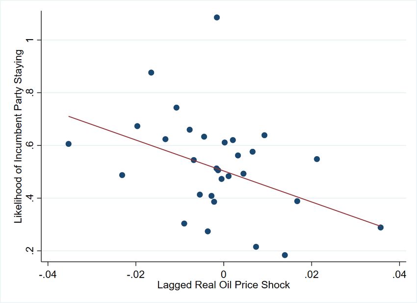
Figure 2 shows the binned scatter plot of the result from column (1) of Table 2. The
figure groups observations into 30 equal-sized bins along the horizontal axis. Thus,
each point represents seven election results, on average. Overall, Figure 2 shows that
the relationship between oil price shocks and election turnover is negative, robust,
and not driven by outliers in our data.
As a concrete example, consider the 2011 parliamentary election in Croatia. In
that election, the incumbent Croatian Democratic Union (Prime Minister Jadranka
Kosor) faced the Social Democratic Party of Croatia (with leader Zoran Milanović).
In our data, the corresponding real oil shock is positive and above average, signifying
a price increase for Croatia (an oil importer). Indeed, this election resulted in a
significant loss for the incumbent party, and an absolute majority for the opposition.
Of course, we do not claim that the outcome was uniquely determined by the oil
price shock. However, we document that these exogenous shocks are an important
factor influencing voter behavior around elections.
In Column 2 of Table 2, we test whether the baseline result is driven by the po-
litical orientation of the incumbent. We define two types of political orientation: left
wing (LW) and right-wing (RW). It is noteworthy that the interaction terms between
oil shock and the political orientation of incumbents are both statistically insignifi-
cant. This result implies that, irrespective of their political orientation, incumbents
are vulnerable to oil shocks.
Column 3 shows that the results are also robust when we control for changes in
copper prices, a proxy for global demand shocks (see Hamilton, 2015). In Column
4, we show that oil shocks still sway electoral outcomes even when other macro
variables at current year and one-year prior are controlled for, namely GDP growth,
inflation and unemployment rate.
When controlling for voter turnout and compulsory voting in elections, the base-
line results remain qualitatively and quantitatively similar (Column 5 of Table 2).
Importantly, this specification also controls for whether the election is a snap election
or predetermined. This test addresses the concern that the timing of an election could
be influenced by oil price movements.
The results are robust to dropping large countries that could arguably influence
oil prices (Column 6). In particularly, this specification drops all election from the US,
8Germany, France, and the UK. The results remain essentially unchanged compared
to baseline. An additional concern may be that the results are driven by the mass of
elections over the past decade, and in particular following the Global Financial Crisis
(GFC). In Column 7, we drop all elections after 2007 and test our main specification
again. Even though this reduces our sample, the results remain robust and highly sig-
nificant. The main findings are not driven by excessive volatility in international oil
prices over the last decade. Nevertheless, we also find a significant negative relation-
ship between oil price shocks and incumbency in the years since the GFC (available
on request).
The main result is also robust and quantitatively similar to using the lagged
change of the import commodity index, consisting of 45 import commodity prices
(Column 8). A 1% increase in import commodity index in the previous year is asso-
ciated with about 11 percentage point increase in the likelihood that the incumbent
party will lose the election.
Finally, in Column 9 we show that a crude oil shock is not only more likely to cause
electoral turnover, but it may also cause a reversal in political leaning. In particular,
we use an indicator for different types of ideological transitions. A transition is
defined as any instance where the incumbent and election winners have a different
ideology (i.e. left-wing versus right-wing). The result in Column 9 shows that oil
shocks are associated with a reversal in political orientation. A 1% increase in oil
price shock leads to a six percentage points increase in the likelihood that the winning
party belongs to the other end of the political spectrum. In other words, following
an oil price increase, a left-leaning incumbent party is more likely to be replaced by a
right-leaning party and vice versa. It is as if voters punish the incumbent party and
would like a wholesale change in political orientations.
Oil price shocks reduce consumption growth, suggesting one potential mechanism
through which oil shocks affect voting behavior. Columns (1)-(2) in Table 3 shows
the regression results using data on per capita final consumption by household and
non-profit institutions serving households. The results suggest that oil shocks in
the previous period have a significant negative effect on lagged private consumption
growth. This reduction could provide an explanation for why voters react so strongly
against incumbents in upcoming elections. Meanwhile, Columns (3)-(4) show that
there is no corresponding effect of oil shocks on lagged GDP growth, suggesting that
the main mechanism works through the consumption channel, not output.
94 Robustness Checks
Our baseline results survive a number of additional robustness checks. First, a
key contribution of this dataset is polling data leading up to every election. In Table
A3 we test for the effects of oil shocks on the voting intention for the incumbent party
in the polls, as outlined in Equation 3. For example, Column (1) shows that for each
election, a 1% increase in the crude oil index 12 months ago reduces voter’s intention
to reelect incumbent party by almost 0.5 percentage points. The effect is not large in
magnitude, but in close elections, even small effects may be important on the margin.
Thus, the fluctuations in oil prices shift the political fortunes of the incumbent party
leading up to the vote, consistent with our main results.
Table A4 shows that when the contemporaneous effect and annual lags of oil
shocks are used, the one-year lag is the only one that causes significant electoral
turnover. Table A5 confirms this finding. It further suggests that when different
quarterly lags are used (up to right quarters before the elections), only oil shocks
four and five quarters before elections are statistically significantly correlated with
the change of power. This period may best coincide with the electoral cycle, though
further research is needed to ascertain this hypothesis. The magnitude is also much
larger than that of the annual lags. For example, a 1% increase in crude oil index a
year (four quarters) before an election reduces the reelection chance by 26 percentage
points.
Finally, Table A6 tests for non-linear effects of oil shocks, as it is possible that
larger oil shocks could have disproportionately larger impacts on electoral outcomes.
However, the quadratic term of oil shocks is not significant, suggesting an absence of
non-linear effects.
5 Conclusion
To our knowledge, this paper is the first to analyze the effect of oil price shocks
on electoral outcomes. The results show that an oil price increase systematically
lowers the odds of reelection for incumbents while increasing the likelihood of an
ideology reversal. These shocks are associated with worsening polling performance
for incumbents in the run-up to elections. We provide evidence that oil price increases
lead to lower consumption growth, and suggest that this may be the mechanism
through which these shocks affect voter behavior.
10The systematic nature of the bias against the incumbent irrespective of political
leaning suggests a rejection of the often-argued voting patterns on the basis of ide-
ology. Our results are consistent with the research on voter retrospection, and con-
tribute to an extensive literature on the economic and political effects of commodity
price fluctuations.
11References
Achen, C. and L. Bartels (2017). Democracy for Realists: Why Elections Do Not Produce
Responsive Government. Princeton University Press.
Aidt, T. S., F. J. Veiga, and L. G. Veiga (2011). Election results and opportunistic poli-
cies: A new test of the rational political business cycle model. Public Choice 148(1-2),
21–44.
Akhmedov, A. and E. Zhuravskaya (2004). Opportunistic political cycles: test in a
young democracy setting. The Quarterly Journal of Economics 119(4), 1301–1338.
Alesina, A. and H. Rosenthal (1995). Partisan Politics, Divided Government and the
Economy. Cambridge University Press.
Alesina, A., N. Roubini, and G. Cohen (1997). Political Cycles and the Macroeconomy.
MIT Press.
Andersen, J. J. and S. Aslaksen (2013). Oil and political survival. Journal of Development
Economics 100, 89–106.
Bakker, R., D. V. Catherine, E. Edwards, L. Hooghe, J. Seth, G. Marks, J. Polk, J. Rovny,
M. Steenbergen, and M. A. Vachudova (2015). Measuing party positions in europe:
The chapel hill expert survey trend file, 1999-2010. Party Politics 21(1), 143–152.
Bazzi, S. and C. Blattman (2014). Economic shocks and conflict: Evidence from com-
modity prices. American Economic Journal: Macroeconomics 6(4), 1–38.
Benoit, K. and M. Laver (2006). Party policy in modern democracies. Routledge research
in comparative politics. Routledge.
Blanchard, O. J. and J. Gali (2009). The macroeconomic effects of oil price shocks:
Why are the 2000s so different from the 1970s? In J. Gali and M. Gertler (Eds.),
International Dimensions of Monetary Policy, pp. 373–428. University of Chicago Press.
Bruckner, M. and A. Ciccone (2010). International commodity prices, growth and the
outbreak of civil war in sub-saharan africa. The Economic Journal 120(544), 519–534.
Bruckner, M., A. Ciccone, and A. Tesei (2012). Oil price shocks, income, and democ-
racy. The Review of Economics and Statistics 94(2), 389–399.
12Burke, P. J. and A. Leigh (2010). Do output contractions trigger democratic change?
American Economic Journal: Macroeconomics 2(4), 124–157.
Caselli, F. and A. Tesei (2016). Resource windfalls, political regimes, and political
stability. The Review of Economics and Statistics 98(3), 573–590.
Castles, F. G. and P. Mair (1984). Left-right political scales: Some ’expert’ judgments.
European Journal of Political Research 12, 73–88.
Cole, S., A. Healy, and E. Werker (2012). Do voters demand responsive governments?
evidence from indian disaster relief. Journal of Development Economics 97, 167–181.
Döring, H. and P. Manow (2019). Parliaments and governments database (parlgov):
Information on parties, elections and cabinets in modern democracies. Technical
report.
Dube, O. and J. F. Vargas (2013). Commodity price shocks and civil conflict: Evidence
from colombia. The Review of Economic Studies 80(4), 1384–1421.
Gasper, J. T. and A. Reeves (2011). Make it rain? retrospection and the attentive elec-
torate in the context of natural disasters. American Journal of Political Science 55(2),
340–355.
Gruss, B. and S. Kebhaj (2019). Commodity terms of trade: a new database. IMF
Working Paper 19/21.
Hamilton, J. (2003). What is an oil shock? Journal of Econometrics 113(2), 363–398.
Hamilton, J. (2015). Demand factors in the collapse of the oil prices. Online.
Healy, A. and N. Malhotra (2010). Random events, economic losses, and retrospec-
tive voting: Implications for democratic competence. Quarterly Journal of Political
Science 5(2), 193–208.
Healy, A. and N. Malhotra (2013). Retrospective voting reconsidered. The Annual
Review of Political Science.
Huber, J. and R. Inglehart (1995). Expert interpretations of party space and party
locations in 42 societies. Party Politics 1(1), 73–111.
van der Ploeg, F. (2011). Natural resources: Curse of blessing? Journal of Economic
Literature 49(2), 366–429.
13Wang, C.-P. and A. Berdiev (2015). Do natural disasters increase the likelihood that a
government is replaced. Applied Economics 17, 1788–1808.
146 Figures
Figure 1: Number of Elections by Year
Notes: This figure presents the number of elections in year of the sample.
Figure 2: Partial Correlation Scatterplot
Notes: Binned scatterplot with 30 equal-sized bins. The full sample contains 207 elections. Year and Country fixed effects are
residualized to produce the figure.
157 Tables
Table 1: Summary Statistics for Main Variables
Variable Count Mean Standard 25 Pctile 50 Pctile 75 Pctile
Deviation
.
Real Oil Shock 198 -.001638 .0252184 -.0144295 .0008879 .0100226
Nominal Oil Shock 198 -.0014319 .0261631 -.0137416 .0011724 .0109492
∆ ln(Import ComPI)t−1 202 -.0009198 .0145936 -.0051851 .0008016 .007443
Indicator: Incumbent Stays 207 .5120773 .5010659 0 1 1
16Table 2: Changes in Crude Oil Prices and Electoral Turnover
(1) (2) (3) (4) (5) (6) (7) (8) (9)
Dependent variable: =1 Incumbent Stays =1 Ideology
Transition
Oil Shock Specification: 3-Year MA 3-Year MA
Real Oil Shockt−1 -5.875∗∗∗ -8.587∗∗∗ -3.660∗∗∗ -4.964∗ -5.810∗∗∗ -5.929∗∗ -25.435∗∗ 6.020∗∗∗
(2.125) (2.696) (1.201) (2.540) (2.081) (2.408) (8.963) (2.098)
∆ ln(Import ComPI)t−1 -11.452∗∗
(5.481)
=1 LW Incumbent -0.095
(0.059)
Real Oil Shockt−1 X LW Incumbent 5.648
(3.606)
∆ ln(Copper Price) -0.354∗
(0.180)
GDP Growtht 0.010
(0.031)
GDP Growtht−1 0.029
(0.018)
Inflationt -0.010
(0.009)
17
Inflationt−1 0.004
(0.004)
∆(Unemployment Rate)t 0.005
(0.061)
∆(Unemployment Rate)t−1 -0.049
(0.054)
Voter Turnout -0.006
(0.007)
=1 Compulsory Voting Election 0.164
(0.372)
=1 Snap Election -0.048
(0.092)
Year FE X X X X X X X X
Country FE X X X X X X X X X
Dropping Large Importers X
Dropping post-GFC Elections X
R2 0.451 0.472 0.355 0.491 0.454 0.481 0.703 0.447 0.437
Mean Dependent Variable 0.511 0.511 0.515 0.514 0.511 0.494 0.581 0.511 0.375
Number of Elections 184 184 194 181 184 160 31 190 184
Number of Countries 47 47 47 46 47 43 11 47 47
Notes: In all columns, oil import exposure is the 3-year rolling average, from t-3 to t-1, of oil imports as a share of GDP. Standard errors are clustered at the country
level and reported in parentheses, stars indicate *** p < 0.01, ** p < 0.05, * p < 0.1.Table 3: Oil Price Shocks, Consumption Growth, GDP Growth
(1) (2) (3) (4)
Dependent variable: ∆ ln(Final Consumption)t−1 GDP Growth(% Change)t−1
Oil Shock Specification: 3-Year MA 3-Year MA
Real Oil Shockt−1 -0.362∗∗ 2.909
(0.153) (14.654)
Real Oil Shockt−2 0.318 -13.216
(0.204) (19.550)
Real Oil Shockt−3 -0.100 -1.034
(0.215) (17.230)
Nominal Oil Shockt−1 -0.321∗∗ 6.918
(0.135) (14.435)
Nominal Oil Shockt−2 0.295 -14.896
(0.189) (18.902)
Nominal Oil Shockt−3 -0.120 -3.562
(0.202) (16.784)
Year FE X X X X
Country FE X X X X
R2 0.567 0.565 0.586 0.588
Mean Dependent Variable 0.019 0.019 2.714 2.714
Number of Elections 179 179 182 182
Number of Countries 46 46 47 47
Notes: The dependent variable in Columns (1)-(2) is log change in Households and NPISHs Final con-
sumption expenditure per capita (constant 2010 USD). In all columns, oil import exposure is the 3-year
rolling average, from t-3 to t-1, of oil imports as a share of GDP. Standard errors are clustered at the country
level and reported in parentheses, stars indicate *** p < 0.01, ** p < 0.05, * p < 0.1.
18Online Appendix
Reversal of Fortune for Political Incumbents:
Evidence from Oil Shocks
Rabah Arezki, Simeon Djankov, Ha Nguyen, Ivan Yotzov
January, 2021
Our analysis draws on two main datasets. The first covers election polls and
outcomes for 207 elections across 50 countries worldwide over the period 1980-2020.
On average, each country has four election cycles. There are 149 parliamentary and
58 presidential elections. The list of countries and the number of elections in each
country by year are presented in the Table A1 and Figure 1.
Table 1 provides summary statistics for the key variables. For an average election,
the average oil shock in real terms is 0.16 percent, and 0.14 percent in nominal terms.
In 51 percent of the elections, the incumbent party wins the election.
Our baseline results survive a battery of other robustness checks. First, the polling
data analyses yield similar results (Table A3). For example, Column (1) shows that for
each election, a 1% increase in the crude oil index 12 months ago reduces a voter’s in-
tention to reelect the incumbent party by 0.5 percentage points. Thus, the fluctuations
in oil prices shift the political fortunes of the incumbent party.
Table A6 tests for non-linear effects of oil shocks, as it is possible that larger oil
shocks could have disproportionately larger impacts on electoral outcomes. However,
the quadratic term of oil shocks is not significant, suggesting an absence of non-linear
effects.
1A Tables
Table A1: Election and Polling Data by Country
Country Number of Elections
argentina 4
australia 12
austria 5
belgium 1
brazil 2
bulgaria 4
canada 5
chile 3
colombia 4
croatia 3
cyprus 3
czech republic 8
denmark 3
ecuador 4
estonia 2
finland 3
france 4
germany 4
greece 5
hungary 4
iceland 4
india 2
ireland 2
italy 3
japan 3
korea, republic of 2
malta 2
mexico 1
netherlands 2
new zealand 6
norway 3
paraguay 2
peru 4
philippines 3
poland 8
portugal 11
romania 3
russian federation 6
serbia 3
slovakia 3
slovenia 4
south africa 2
spain 8
sweden 4
switzerland 3
taiwan, province of china 4
turkey 5
united kingdom 9
united states 10
uruguay 2
Total 207
2Table A2: Oil Price Shocks and Alternative Standard Error Clustering
(1) (2) (3) (4)
Dependent variable: =1 Incumbent Stays
Oil Shock Specification: 3-Year MA 5-Year MA
Real Oil Shockt−1 -5.875∗∗∗ -7.832∗∗∗
(1.849) (2.551)
Nominal Oil Shockt−1 -5.450∗∗∗ -7.101∗∗∗
(1.737) (2.445)
Country FE X X X X
Year FE X X X X
R2 0.451 0.450 0.441 0.440
Mean Dependent Variable 0.511 0.511 0.511 0.511
Number of Elections 184 184 182 182
Number of Countries 47 47 47 47
Notes: Standard errors are clustered at the country and year level and reported in
parentheses, stars indicate *** p < 0.01, ** p < 0.05, * p < 0.1.
Table A3: Oil Price Shocks and Polling Data
(1) (2) (3) (4)
Dependent variable: Voting Intention for Incumbent
Oil Shock Specification: 3-Year MA 5-Year MA
Oil Shockt−12 -49.155∗∗ -21.760∗∗ -59.152∗ -28.926∗
(22.177) (9.948) (32.661) (14.711)
Month FE X X X X
Country FE X X
Election FE X X
R2 0.710 0.936 0.709 0.935
Mean Dependent Variable 33.721 33.721 33.641 33.641
Observations 2,354 2,354 2,331 2,331
Number of Elections 189 189 187 187
Notes: Voting intention captures the percentage of voters intending to vote for the
incumbent party. In columns (1) and (2), oil import exposure is the 3-year rolling
average, from t-3 to t-1, of oil imports as a share of GDP. In columns (3) and (4), oil
import exposure is the 5-year rolling average, from t-5 to t-1, of oil imports as a share
of GDP. The poll sample includes the actual elections as well. Standard errors are
clustered at the country level and reported in parentheses, stars indicate *** p < 0.01,
** p < 0.05, * p < 0.1.
3Table A4: Oil Price Shocks with Annual Lags
(1) (2)
Dependent variable: =1 Incumbent Stays
Oil Shock Specification: Real Shock Nominal Shock
Oil Shockt -1.670 -2.106
(3.183) (2.780)
Oil Shockt−1 -7.168∗∗ -6.036∗∗
(3.060) (2.898)
Oil Shockt−2 4.941 4.106
(4.754) (4.343)
Oil Shockt−3 -6.539 -6.577
(4.929) (4.246)
Country FE X X
Year FE X X
R2 0.461 0.461
Mean Dependent Variable 0.511 0.511
Number of Elections 182 182
Number of Countries 47 47
Notes: Oil shocks calculated using international crude oil prices
weighted by 3-year rolling windows of oil import to GDP value for
each country. Annual lags are included. For example, Oil Shock t−1 is
the Crude Oil Shock one year before the election. Standard errors are
clustered at the country level and reported in parentheses, stars indicate
*** p < 0.01, ** p < 0.05, * p < 0.1.
4Table A5: Oil Price Shocks with Quarterly Lags
(1) (2)
Dependent variable: =1 Incumbent Stays
Oil Shock Specification: 3-Year MA 5-Year MA
Oil Shockt -0.076 -3.689
(7.868) (7.683)
Oil Shockt−1 -0.363 -1.537
(7.436) (12.977)
Oil Shockt−2 14.077 11.928
(8.451) (8.307)
Oil Shockt−3 -3.118 -1.777
(4.937) (8.478)
Oil Shockt−4 -26.788∗∗∗ -19.942∗∗
(8.949) (9.145)
Oil Shockt−5 -11.004∗∗∗ -2.014
(4.030) (7.609)
Oil Shockt−6 -3.108 7.257
(3.622) (5.349)
Oil Shockt−7 3.129 1.838
(6.407) (6.890)
Oil Shockt−8 4.047 5.388
(4.663) (7.150)
Country FE X X
Quarter FE X X
R2 0.730 0.697
Mean Dependent Variable 0.510 0.503
Observations 151 149
Number of Elections 43 43
Notes: Oil shocks calculated using international crude oil prices
weighted by 3-year rolling windows of oil import to GDP value
for each country. Quarterly lags are included. For example,
Oil Shock t−1 is Crude Oil Shocks one quarter before the election.
Standard errors are clustered at the country level and reported in
parentheses, stars indicate *** p < 0.01, ** p < 0.05, * p < 0.1.
5Table A6: Non-Linear Effects of Oil Price Shocks
(1) (2) (3) (4)
Dependent variable: =1 Incumbent Stays
Oil Shock Specification: 3-Year MA 5-Year MA
Real Oil Shockt−1 -4.932∗∗ -7.698∗∗
(2.327) (3.537)
Real Oil Shock2t−1 48.126 94.995
(30.935) (119.447)
Nominal Oil Shockt−1 -4.593∗∗ -7.154∗
(2.263) (3.601)
Nominal Oil Shock2t−1 42.566 108.084
(27.056) (104.200)
Year FE X X X X
Country FE X X X X
R2 0.457 0.455 0.444 0.444
Mean Dependent Variable 0.511 0.511 0.511 0.511
Number of Elections 184 184 182 182
Number of Countries 47 47 47 47
Notes: Standard errors are clustered at the country level and reported in parentheses,
stars indicate *** p < 0.01, ** p < 0.05, * p < 0.1.
6You can also read