Reviews and syntheses: Turning the challenges of partitioning ecosystem evaporation and transpiration into opportunities - Biogeosciences
←
→
Page content transcription
If your browser does not render page correctly, please read the page content below
Biogeosciences, 16, 3747–3775, 2019
https://doi.org/10.5194/bg-16-3747-2019
© Author(s) 2019. This work is distributed under
the Creative Commons Attribution 4.0 License.

Reviews and syntheses: Turning the challenges of partitioning
ecosystem evaporation and transpiration into opportunities
Paul C. Stoy1,2 , Tarek S. El-Madany3 , Joshua B. Fisher4,5 , Pierre Gentine6 , Tobias Gerken7 , Stephen P. Good8 ,
Anne Klosterhalfen9 , Shuguang Liu10 , Diego G. Miralles11 , Oscar Perez-Priego3,12 , Angela J. Rigden13 ,
Todd H. Skaggs14 , Georg Wohlfahrt15 , Ray G. Anderson14 , A. Miriam J. Coenders-Gerrits16 , Martin Jung3 ,
Wouter H. Maes11 , Ivan Mammarella17 , Matthias Mauder18 , Mirco Migliavacca3 , Jacob A. Nelson3 ,
Rafael Poyatos19,20 , Markus Reichstein3 , Russell L. Scott21 , and Sebastian Wolf22
1 Department    of Biological Systems Engineering, University of Wisconsin-Madison, Madison, WI 53706, USA
2 Department    of Land Resources and Environmental Sciences, Montana State University, Bozeman, MT 59717, USA
3 Max Planck Institute for Biogeochemistry, Hans Knöll Straße 10, 07745 Jena, Germany
4 Jet Propulsion Laboratory, California Institute of Technology, 4800 Oak Grove Drive, Pasadena, CA 91109, USA
5 Joint Institute for Regional Earth System Science and Engineering, University of California at Los Angeles,

Los Angeles, CA 90095, USA
6 Department of Earth and Environmental Engineering, Columbia University, New York, NY 10027, USA
7 The Pennsylvania State University, Department of Meteorology and Atmospheric Science, 503 Walker Building,

University Park, PA, USA
8 Department of Biological & Ecological Engineering, Oregon State University, Corvallis, Oregon, USA
9 Agrosphere Institute, IBG-3, Forschungszentrum Jülich GmbH, 52425 Jülich, Germany
10 National Engineering Laboratory for Applied Technology of Forestry and Ecology in South China,

Central South University of Forestry and Technology, Changsha, China
11 Laboratory of Hydrology and Water Management, Ghent University, Coupure Links 653, 9000 Gent, Belgium
12 Department of Biological Sciences, Macquarie University, North Ryde, NSW 2109, Australia
13 Department of Earth and Planetary Sciences, Harvard University, Cambridge, MA 02138, USA
14 U.S. Salinity Laboratory, USDA-ARS, Riverside, CA, USA
15 Institut für Ökologie, Universität Innsbruck, Sternwartestr. 15, 6020 Innsbruck, Austria
16 Water Resources Section, Delft University of Technology, Stevinweg 1, 2628 CN Delft, the Netherlands
17 Institute for Atmospheric and Earth System Research/Physics, Faculty of Science, 00014 University of Helsinki,

Helsinki, Finland
18 Karlsruhe Institute of Technology, Institute of Meteorology and Climate Research – Atmospheric Environmental Research,

Garmisch-Partenkirchen, Germany
19 CREAF, E08193 Bellaterra (Cerdanyola del Vallès), Catalonia, Spain
20 Laboratory of Plant Ecology, Faculty of Bioscience Engineering, Ghent University, Coupure links 653,

9000 Ghent, Belgium
21 Southwest Watershed Research Center, USDA Agricultural Research Service, Tucson, AZ, USA
22 Department of Environmental Systems Science, ETH Zurich, Zurich, Switzerland

Correspondence: Tarek S. El-Madany (telmad@bgc-jena.mpg.de)

Received: 7 March 2019 – Discussion started: 12 March 2019
Revised: 20 August 2019 – Accepted: 22 August 2019 – Published: 1 October 2019

Published by Copernicus Publications on behalf of the European Geosciences Union.
3748 P. C. Stoy et al.: Reviews and syntheses: Ecosystem evaporation and transpiration
Abstract. Evaporation (E) and transpiration (T ) respond dif- up to 50 % (Mao et al., 2015; Vinukollu et al., 2011). LSMs
ferently to ongoing changes in climate, atmospheric compo- also struggle to simulate the magnitude and/or seasonality
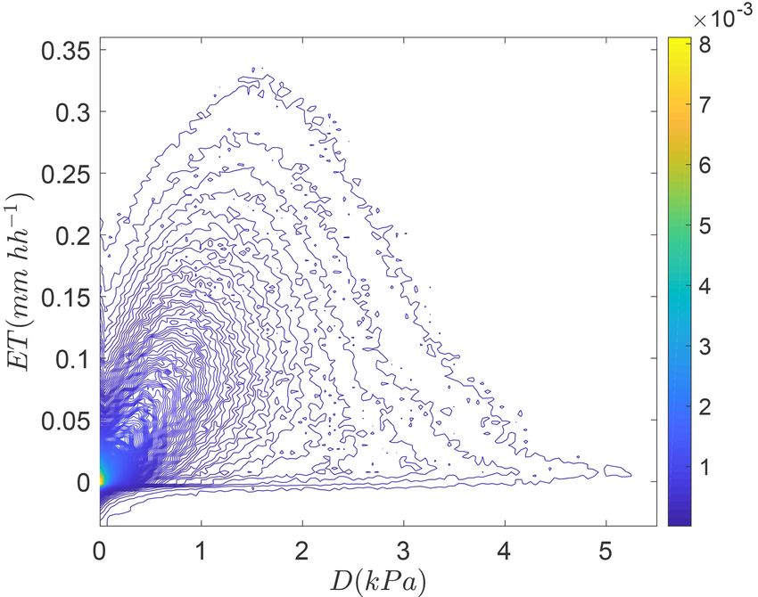
sition, and land use. It is difficult to partition ecosystem-scale of ET at the ecosystem scale (Fig. 1), suggesting fundamen-
evapotranspiration (ET) measurements into E and T , which tal gaps in our understanding of the terrestrial water cycle.
makes it difficult to validate satellite data and land surface These issues need to be resolved to effectively manage wa-
models. Here, we review current progress in partitioning E ter resources as climate continues to change (Dolman et al.,
and T and provide a prospectus for how to improve the- 2014; Fisher et al., 2017).
ory and observations going forward. Recent advancements in Along with technological and data limitations, we ar-
analytical techniques create new opportunities for partition- gue that a fundamental challenge in modeling ET at the
ing E and T at the ecosystem scale, but their assumptions global scale is difficulty measuring transpiration (T ) through
have yet to be fully tested. For example, many approaches plant stomata and evaporation (E) from non-stomatal sur-
to partition E and T rely on the notion that plant canopy faces at the ecosystem scale (Fisher et al., 2017; McCabe
conductance and ecosystem water use efficiency exhibit op- et al., 2017). LSMs and remote sensing algorithms (see Ap-
timal responses to atmospheric vapor pressure deficit (D). pendix A) rely on a process-based understanding of E and T
We use observations from 240 eddy covariance flux towers to estimate ET, but it is not clear how to guide their improve-
to demonstrate that optimal ecosystem response to D is a ment without accurate ground-based E and T observations at
reasonable assumption, in agreement with recent studies, but spatial scales on the order of a few kilometers or less (Talsma
more analysis is necessary to determine the conditions for et al., 2018) and temporal scales that capture diurnal, sea-
which this assumption holds. Another critical assumption for sonal, and interannual variability in water fluxes. Recent sta-
many partitioning approaches is that ET can be approximated tistical ET partitioning approaches (Rigden et al., 2018) are
as T during ideal transpiring conditions, which has been similarly limited by the lack of direct E and T observations
challenged by observational studies. We demonstrate that T for evaluation. Interest in partitioning E and T from ecosys-
can exceed 95 % of ET from certain ecosystems, but other tem ET measurements has grown in recent years (Anderson
ecosystems do not appear to reach this value, which sug- et al., 2017b), and many new measurements and modeling
gests that this assumption is ecosystem-dependent with im- approaches seek to do so but often rely on assumptions that
plications for partitioning. It is important to further improve need further testing. We begin with a brief research review
approaches for partitioning E and T , yet few multi-method that notes recent updates to our theoretical understanding of
comparisons have been undertaken to date. Advances in our ET and outlines the challenges in measuring E and T at the
understanding of carbon–water coupling at the stomatal, leaf, ecosystem scale. We then describe current and emerging in-
and canopy level open new perspectives on how to quantify novations in partitioning E and T (Table 1) and use observa-
T via its strong coupling with photosynthesis. Photosynthe- tions to challenge some of the assumptions upon which these
sis can be constrained at the ecosystem and global scales approaches rely. We finish with an outlook of how carefully
with emerging data sources including solar-induced fluores- designed ecosystem-scale experiments can constrain models
cence, carbonyl sulfide flux measurements, thermography, of E and T to improve our understanding going forward.
and more. Such comparisons would improve our mechanistic
understanding of ecosystem water fluxes and provide the ob-
servations necessary to validate remote sensing algorithms 2 Background
and land surface models to understand the changing global
water cycle. 2.1 Vegetation plays a central role in evaporation and
transpiration partitioning
The ratio of transpiration to evapotranspiration (T / ET) at
1 Introduction annual timescales is related to aridity (Good et al., 2017)
but appears to be relatively insensitive to annual precipita-
Some 70 000 km3 of water leaves terrestrial ecosystems and tion (P ) (Schlesinger and Jasechko, 2014). T / ET is sensi-
enters the atmosphere through evapotranspiration (ET) every tive to ecosystem characteristics, namely the leaf area index
year (Jung et al., 2019; Oki and Kanae, 2006). Despite its (LAI) (Berkelhammer et al., 2016; Fatichi and Pappas, 2017;
importance, we are unsure whether global ET has been in- Wang et al., 2014; Wei et al., 2015), especially on sub-annual
creasing over time (Brutsaert, 2013, 2017; Brutsaert and Par- timescales (Li et al., 2019; Scott and Biederman, 2017), not-
lange, 1998; Zeng et al., 2018; Zhang et al., 2016) such that ing that LAI is related to P at longer timescales. A higher
the water cycle is accelerating (Ohmura and Wild, 2002) or LAI favors T and E from intercepted water (Ei ) at the ex-
decreasing and causing more river discharge (Gedney et al., pense of E from soil (Esoil ) such that LAI explains some
2006; Labat et al., 2004; Probst and Tardy, 1987). Global ET 43 % of the variability of annual T / ET across global ecosys-
volumes from reanalyses, upscaled estimates, and land sur- tems (Wang et al., 2014). Upscaling this relationship results
face model (LSM) outputs disagree (Mueller et al., 2013) by in a global estimate of terrestrial annual T / ET of 0.57±0.07
Biogeosciences, 16, 3747–3775, 2019 www.biogeosciences.net/16/3747/2019/
P. C. Stoy et al.: Reviews and syntheses: Ecosystem evaporation and transpiration                                                      3749

Figure 1. The mean monthly latent heat flux (λE) – the energy used for evapotranspiration – from eddy covariance measurements from four
research sites (“MEASURED”) and 13 ecosystem models from the North American Carbon Program Site-Level Interim Synthesis (Schwalm
et al., 2010). Sites: CA-Ca1 (Schwalm et al., 2007), CA-Obs (Griffis et al., 2003; Jarvis et al., 1997), US-Ho1 (Hollinger et al., 1999), US-
Me2 (Thomas et al., 2009). Models: BEPS (Liu et al., 1999), CAN-IBIS (Williamson et al., 2008), CNCLASS (Arain et al., 2006), ECOSYS
(Grant et al., 2005), ED2 (Medvigy et al., 2009), ISAM (Jain and Yang, 2005), ISOLSM (Riley et al., 2002), LOTEC (Hanson et al., 2004),
ORCHIDEE (Krinner et al., 2005), SIB (Baker et al., 2008), SIBCASA (Schaefer et al., 2009), SSIB2 (Zhan et al., 2003), TECO (Weng and
Luo, 2008). Data are available from Ricciuto et al. (2013).

(Wei et al., 2017). Other observational studies suggest that             of T / ET is the treatment of lateral flow in models (Chang
annual T / ET averages nearly 2/3 globally (0.61 ± 0.15,                 et al., 2018). Explicitly adding lateral flow and groundwa-
Schlesinger and Jasechko, 2014; 0.64 ± 0.13, Good et al.,                ter dynamics is critical for accurate T estimation (Maxwell
2015; and 0.66 ± 0.13 across some FLUXNET sites, Li et                   and Condon, 2016), and realistic lateral flow results in lower
al., 2019). Intercomparison studies agree on the large un-               E (Chang et al., 2018; Ji et al., 2017). Simulating sub-grid
certainty surrounding these estimates, with reported global              water partitioning is often of particular importance during
terrestrial annual T / ET ratios ranging from 0.35 to 0.90               drought (Ji et al., 2017; Shrestha et al., 2018), as is a realistic
(Coenders-Gerrits et al., 2014; Fatichi and Pappas, 2017;                representation of plant water stress parameters (Fang et al.,
Young-Robertson et al., 2018). Approaches that use stable                2017). In addition to challenges in simulating T / ET across
isotopes tend to produce higher annual T / ET values due                 space, we also need to measure and model T / ET correctly at
to assumptions regarding isotopic fractionation (Jasechko et             the ecosystem scale across all timescales over which it varies
al., 2013; Sutanto et al., 2014). Some LSM estimates of an-              from minutes or less to multiple years or more. For this, an
nual T / ET arrive at larger values on the order of 0.70±0.09            understanding of ecosystem water transport and biological
(Fatichi and Pappas, 2017; Paschalis et al., 2018), while other          responses to micrometeorological forcing is necessary (Bad-
LSMs suggest smaller T / ET; for example, T / ET from the                gley et al., 2015).
IPCC CMIP5 intercomparison ranges from 0.22 to 0.58 (Wei
et al., 2017). Constraining these model results with observa-            2.2   Turning theory into practice
tions results in an estimate similar to observational studies
but with reduced uncertainty: 0.62 ± 0.06 (Lian et al., 2018).           Measuring and modeling water fluxes from the surface to
A number of recent studies suggest that a major cause of                 the atmosphere at the ecosystem scale across multiple scales
the discrepancies between observations and LSM predictions               in time is a nontrivial challenge. The pools in which wa-
                                                                         ter is stored in ecosystems span spatial scales from soil

www.biogeosciences.net/16/3747/2019/                                                              Biogeosciences, 16, 3747–3775, 2019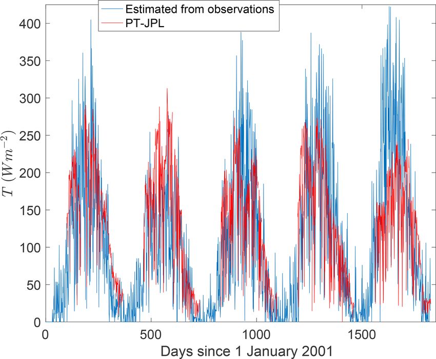
3750                                       P. C. Stoy et al.: Reviews and syntheses: Ecosystem evaporation and transpiration

Table 1. A summary of recent approaches for estimating transpiration (T ) and/or for partitioning evapotranspiration (ET) into evaporation (E)
and T at the ecosystem scale. The reader is referred to Kool et al. (2014) for a comprehensive review of E and T measurement methodologies.

 Approach                Advantages                             Disadvantages                           Selected references
 Flux–variance           Uses high-frequency eddy covari-       Necessary terms rarely computed         Scanlon and Kustas (2010), Scan-
 similarity              ance data; open-source software is     and/or high-frequency data to cal-      lon and Sahu (2008), Skaggs et al.
                         available                              culate terms are rarely shared; sen-    (2018)
                                                                sitive to water use efficiency as-
                                                                sumptions
 Analyses of             Use widely available eddy covari-      Often rely on assumptions regard-       Berkelhammer et al. (2016), Lin et
 half-hourly to          ance data                              ing water use efficiency and the        al. (2018), Li et al. (2019), Scott
 hourly eddy                                                    maximum value of the T / ET ratio       and Biederman (2017), Zhou et al.
 covariance data                                                                                        (2016)
 Solar-induced           Measurements are available at          Relies on an empirical relationship     Damm et al. (2018), Lu et al.
 fluorescence            ecosystem to global scales             between T and gross primary pro-        (2018), Shan et al. (2019)
                                                                ductivity; mechanistic link not yet
                                                                understood; uncertainty in SIF re-
                                                                trieval
 Carbonyl sulfide        Can be measured using eddy co-         COS flux can also arise from non-       Whelan et al. (2018), Wohlfahrt et
 (COS) flux              variance techniques to estimate        stomatal sources                        al. (2012)
                         canopy conductance
 Surface evaporative     Based on the theory of Esoil and can   Applies only to Esoil                   Or and Lehman (2019)
 capacitance             be estimated using remote sensing

pores to forest canopies. Liquid and gaseous water trans-                Esoil , and conductance related to plant-intercepted evapora-
port occurs through pathways in the soil, xylem, leaves, and             tion (gi ) associated with Ei . The combination of Esoil and
plant surfaces that exhibit nonlinear responses to hydrocli-             Ei results in ecosystem-scale E. The biological drivers that
matic forcing, which is itself stochastic (Katul et al., 2007,           alter gc impact T , but physical drivers impact both E and
2012). These complex dynamics of water storage and trans-                T . In practice, the Penman–Monteith equation is commonly
port impact the conductance of water between ecosystems                  simplified because of the challenge of correctly simulating
and the atmosphere (Mencuccini et al., 2019; Siqueira et                 all relevant conductances (Maes et al., 2019; Priestley and
al., 2008), and these conductance terms are central to the               Taylor, 1972).
Penman–Monteith equation, which combines the thermody-                      The micrometeorological drivers of the Penman–Monteith
namic, aerodynamic, environmental, and biological variables              equation vary within and across plant canopies and land-
to which ET (m s−1 ) responds to represent the mass and en-              scapes (Jarvis and McNaughton, 1986), as do the turbulent
ergy balance of water flux between the land surface and the              structures that transport water into the atmosphere by which
atmosphere (Monteith, 1965; Penman, 1948):                               ET can be measured using eddy covariance. Because ET
                                                                         is commonly measured above plant canopies with eddy co-
        1 s (Rn − G) + ρa cp Dga
ET =                          .                               (1)      variance, micrometeorological variables are commonly mea-
       ρλ s + γ 1 + ga                                                   sured above plant canopies as well. These measurements
                        gsurf
                                                                         do not necessarily reflect micrometeorological conditions at
In the Penman–Monteith equation, λ is the latent heat of va-             evaporating and transpiring surfaces. For example, character-
porization (J kg−1 ), ρ is the density of water (kg m−3 ), s is          istic profiles of water vapor concentration in the atmosphere
the slope of the saturation vapor pressure function (Pa K−1 ),           measured above the plant canopy are different from D at the
Rn is the surface net radiation (W m−2 ), G is the ground heat           canopy, leaf, and soil levels (De Kauwe et al., 2017; Jarvis
flux (W m−2 ), ρa is dry air density (kg m−3 ), cp is the spe-           and McNaughton, 1986; Lin et al., 2018). Furthermore, the
cific heat capacity of air (J kg−1 K−1 ), D is the vapor pres-           fundamental assumption that D reflects the difference be-
sure deficit (Pa), γ is the psychrometric constant (Pa K−1 ),            tween atmospheric water vapor pressure and saturated condi-
ga is the conductance of the atmosphere, and gsurf is sur-               tions within the leaf is challenged by studies demonstrating
face conductance to water vapor flux (both m s−1 ). gsurf is             that leaf vapor pressure need not be saturated (Cernusak et
a spatially upscaled effective parameter that includes canopy            al., 2018). Radiation, temperature, and wind speed also vary
conductance from stomatal opening (gc ) associated with T ,              throughout plant canopies with consequences for modeling
conductance related to soil evaporation (gsoil ) associated with

Biogeosciences, 16, 3747–3775, 2019                                                             www.biogeosciences.net/16/3747/2019/
P. C. Stoy et al.: Reviews and syntheses: Ecosystem evaporation and transpiration 3751
T from the canopy and E from the soil and other ecosystem
surfaces. The space–time variability of environmental drivers
within plant canopies should therefore ideally be measured
or simulated to understand how they impact E and T , and
ecosystem modelers must decide if this canopy-resolved de-
tail is important to simulate in diverse ecosystems (Boulet et
al., 1999; Medvigy et al., 2009; Polhamus et al., 2013).
Modeling ET at the ecosystem scale is challenging enough
before noting that ongoing changes to the Earth system im-
pact all of the biotic and abiotic variables that determine it.
The decline in incident radiation across some regions of the
world due largely to anthropogenic aerosols (“global dim-
ming”) and subsequent increase since about 1990 (“global
brightening”) have changed incident radiation and thus Rn at
the land surface (Wild et al., 2005). The observed decrease
in wind speed (“global stilling”) (McVicar et al., 2012a, b)
is partly due to increases in surface roughness owing to in- Figure 2. The relationship between above-canopy vapor pressure
creases in LAI (Vautard et al., 2010) and has decreased ga , deficit (D) and evapotranspiration (ET in millimeters per half hour,
hh) visualized using kernel density estimation (Botev et al., 2010)
which is a function of wind speed (Campbell and Norman,
for more than 1.5 million half-hourly eddy covariance observations
1998). Atmospheric heating changes the terms in Eq. (1) that with a solar zenith angle less than 60◦ from 241 eddy covariance
involve temperature, namely Rn (via incident longwave ra- research sites in the La Thuile FLUXNET database that included
diation), λ, γ , and s, through the Clausius–Clapeyron rela- ecosystem type and soil heat flux measurements described in Stoy
tion. A warming climate also increases D in the absence of et al. (2013).
changes in specific humidity, but specific humidity has in-
creased across many global regions (Willett et al., 2008),
resulting in complex spatial and temporal changes in D E and T respond to a range of biotic and abiotic variability
(Ficklin and Novick, 2017). gc is controlled by soil mois- for predictive understanding. To do so, we need to accurately
ture availability (Porporato et al., 2004), plant hydrodynam- measure E and T in the first place.
ics (Bohrer et al., 2005; Matheny et al., 2014), and envi-
ronmental variables including D that result in stomatal clo-
sure (Oren et al., 1999) (Fig. 2), which is critical for mod- 3 Measuring and estimating evaporation and
els to accurately simulate (Rogers et al., 2017). This depen- transpiration
dency on D is predicted to become increasingly important
as global temperatures continue to rise (Novick et al., 2016), There are multiple established methods to measure ecosys-
but D is also highly coupled to soil moisture (Zhou et al., tem E and T , including leaf gas exchange, plant-level
2019), and both depend on ET itself through soil–vegetation– sap flow, lysimeters, soil, leaf, and canopy chambers, pho-
atmosphere coupling. Increases in atmospheric CO2 concen- tometers, soil heat pulse methods, and stable and radioiso-
tration tend to decrease stomatal conductance at the leaf scale topic techniques. Ongoing efforts to synthesize measure-
(Field et al., 1995) and have been argued to decrease gc on ments of ecosystem water cycle components – for example,
a global scale (Gedney et al., 2006). However, elevated CO2 SAPFLUXNET (Poyatos et al., 2016) – are a promising ap-
often favors increases in LAI (e.g., Ellsworth et al., 1996), proach to build an understanding of different terms of the
thus leading to an increase in transpiring area that can sup- ecosystem water balance across global ecosystems. Multi-
port greater gc . Atmospheric pollutants including ozone also ple reviews and syntheses of E and T measurements have
impact gc with important consequences for vegetation func- been written (e.g., Abtew and Assefa, 2012; Anderson et al.,
tion (Hill et al., 1969; Wittig et al., 2007). Water fluxes from 2017b; Blyth and Harding, 2011; Kool et al., 2014; Shut-
the land surface impact atmospheric boundary layer pro- tleworth, 2007; Wang and Dickinson, 2012) and have pro-
cesses including cloud formation, extreme temperatures, and vided the key insights that ecosystem models use to simulate
precipitation (Gerken et al., 2018; Lemordant et al., 2016; ecosystem–atmosphere water flux (De Kauwe et al., 2013).
Lemordant and Gentine, 2018), which feeds back to land sur- Rather than reiterate the findings of these studies, we focus
face fluxes in ways that are inherently nonlinear and difficult on existing and emerging approaches to partition E and T at
to simulate (Ruddell et al., 2013). In addition to these highly the ecosystem scale on the order of tens of meters to kilome-
nonlinear dynamics of the soil–vegetation–atmosphere sys- ters at temporal resolutions on the order of minutes to hours,
tem, ongoing land use and land cover changes impact vege- with a particular emphasis on new observational and method-
tation structure and function with important implications for ological techniques. We do so to align ecosystem-scale ob-
the water cycle. In brief, we need to correctly simulate how servations of E and T with satellite-based algorithms that
www.biogeosciences.net/16/3747/2019/ Biogeosciences, 16, 3747–3775, 20193752 P. C. Stoy et al.: Reviews and syntheses: Ecosystem evaporation and transpiration
can scale E and T from ecosystem to region to globe (Ap-
pendix A).
ET is commonly approximated as the residual of the water
balance at the watershed scale in hydrologic studies – espe-
cially when the change in water storage can be assumed to
be negligible – but can now be measured using eddy covari-
ance at the ecosystem scale (Wilson et al., 2001). Other ap-
proaches including scintillometry (Cammalleri et al., 2010;
Hemakumara et al., 2003), surface renewal (Snyder et al.,
1996), and the Bowen ratio energy balance method provide
important complements to eddy covariance techniques for
measuring ecosystem-scale ET. Such syntheses follow on-
going efforts to compile ET measured by eddy covariance
via FLUXNET and cooperating consortia (Chu et al., 2017),
which synthesize half-hourly to hourly eddy covariance flux
measurements that have been used to partition ET into E and
T with mixed success.
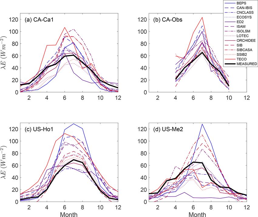
Figure 3. The Priestley–Taylor Jet Propulsion Lab (PT-JPL) esti-
3.1 Partitioning ET using half-hourly eddy covariance mate of transpiration (T ) in energy flux units compared against
observations T estimated using eddy covariance measurements and models of
soil evaporation in a loblolly pine forest for 2001–2005 from Stoy
An early attempt to partition E and T directly from eddy co- et al. (2006). Measurements were taken at 10:30 Eastern Standard
variance measurements assumed that ET is comprised solely Time (UTC−5 h).
of E in the absence of canopy photosynthesis (gross primary
productivity, GPP) due to the coupled flux of carbon and wa-
most work to date has used below-canopy eddy covariance
ter through plant stomata (Stoy et al., 2006). It was further
to partition canopy GPP and soil respiration (Misson et al.,
assumed that Esoil dominated ET during these times and that
2007). Several recent studies demonstrated the additional
Esoil could be modeled by simulating solar radiation attenua-
value of concurrent below-canopy measurements for quan-
tion through grass, pine forest, and deciduous forest canopies
tifying the coupling and decoupling of below- and above-
in the Duke Forest, NC, USA. T was subsequently approxi-
canopy airspace to accurately apply the eddy covariance
mated as the difference between measured ET and the model
technique in forested ecosystems (Jocher et al., 2017, 2018;
for Esoil during times when photosynthesis was active. An-
Paul-Limoges et al., 2017; Thomas et al., 2013), arguing
nual T / ET values from this approach varied from 0.35 to
that below-canopy eddy covariance measurements should be
0.66 in the grass ecosystem (US-Dk1) across a 4-year period
more widely adopted. Other eddy-covariance-based parti-
and between 0.7 and 0.75 in the pine (US-Dk3) and hard-
tioning methods take a different approach and use the rela-
wood (US-Dk2) forests, somewhat higher than global syn-
tionship between T and GPP to partition ecosystem-scale E
theses (Schlesinger and Jasechko, 2014), remote sensing es-
and T .
timates from PT-JPL (see Appendix A) for the Duke pine
Scott and Biederman (2017) assumed that T is linearly re-
forest (Fig. 3), and sap-flow-based measurements from the
lated to GPP at monthly timescales over many years such
deciduous forest (Oishi et al., 2008). These discrepancies
that
arose in part because Ei was considered negligible but can
be considerable (see Sect. 3.6). The model for Esoil could T = mWUE rGPP , (2)
also not be directly validated using measurements from the
forest floor alone with available observations. where mWUE is the inverse of the marginal water use
An under-explored approach for partitioning Esoil from efficiency (the change, 1, in ET per change in GPP:
ecosystem ET uses concurrent above- and below-canopy 1ET/1GPP), and r is the ratio between the inverse of the
eddy covariance measurements in forest and savanna ecosys- transpirational water use efficiency (1T /1GPP) and the
tems (Misson et al., 2007). Subcanopy eddy covariance mea- marginal ecosystem water use efficiency, which is assumed
surements have proven useful for measuring below-canopy to be unity. It follows that the intercept E 0 of the relationship
ET, often assumed to be comprised largely of Esoil in ecosys- ET = mGPP + E 0 is an estimate of average monthly E. This
tems with poor understory cover (Baldocchi et al., 1997; approach is favored in semiarid ecosystems in which there is
Baldocchi and Ryu, 2011; Moore et al., 1996; Sulman et a close coupling of ET and GPP and E makes up a consider-
al., 2016). However, such measurements are not yet widely able amount of monthly ET.
adopted for ET partitioning studies due to a limited under- Several recently developed methods for partitioning eddy-
standing of their performance (Perez-Priego et al., 2017); covariance-measured ET are based on the optimality theory
Biogeosciences, 16, 3747–3775, 2019 www.biogeosciences.net/16/3747/2019/P. C. Stoy et al.: Reviews and syntheses: Ecosystem evaporation and transpiration 3753
assumption that plants minimize water loss per unit of CO2 In a more sophisticated attempt to partition ET utilizing
gain (e.g., Hari et al., 2000; Katul et al., 2009; Medlyn et optimality theory, Perez-Priego et al. (2018) utilized a big-
al., 2011; Schymanski et al., 2007). An outcome of this ap- leaf canopy model in which parameters were optimized using
proach is that plant water use efficiency WUE, defined here half-hourly data in 5-day windows. Uniquely, the marginal
as GPP/T , scales with D 0.5 from which a relationship be- carbon cost of water was factored into the cost function dur-
tween GPP and T can be derived (Katul et al., 2009). Berkel- ing parameter estimation, so the parameters for each 5-day
hammer et al. (2016) noted that ET follows a linear relation- window maximized the fit between modeled and observed
ship to GPP × D 0.5 and further assumed that the T / ET ratio GPP and also minimized water loss per carbon gain. T was
intermittently approaches 1. They then separated ET mea- then calculated using gc from the model, and E was calcu-
surements from eddy covariance into GPP classes for which lated as the residual (ET − T ).
a minimum ET, min (ET) |GPP , can be defined. T / ET can A modified (in this case binned) parameter optimization
then be calculated using approach was used by Li et al. (2019) to estimate gsurf , which
follows the model proposed by Lin et al. (2018):
ET
T / ET = . (3) GPP
min (ET) |GPP gsurf = g0 + g1 . (6)
DLm
Applying this approach to different forests revealed consider- Here, g0 (assumed to correspond to soil conductance), g1
able synoptic-scale variability in T / ET that was dampened (assumed to correspond to vegetation conductance), and m
at seasonal timescales and compared well against isotopic ap- are optimized parameters, DL is the inferred leaf-level D,
proaches (Berkelhammer et al., 2016). and gsurf is estimated by inverting Eq. (1) and is assumed to
Zhou et al. (2016) built upon earlier work (Zhou et al., represent ecosystem conductance to water vapor flux. Rather
2014) and assumed that an ecosystem has an actual underly- than optimizing using a moving window over time, data were
ing water use efficiency (uWUEa , where WUE in this case is binned using independent soil moisture data associated with
defined as GPP/ET), which is maximal or reaches its poten- the eddy covariance site, with g0 , g1 , and m optimized in
tial underlying water use efficiency (uWUEp ) when T / ET each bin to account for changes due to water limitations. Par-
approaches unity. T / ET can thus be calculated from the ra- titioning was then calculated as
tio of actual to potential uWUE using optimality assumptions
T g1
for both: = (7)
ET gsurf
√
GPP D and
uWUEp = (4)
T E g0
= . (8)
and ET gsurf
√ The Perez-Priego et al. (2018) and Li et al. (2019) meth-
GPP D ods both circumvent the assumption that T / ET approaches
uWUEa = . (5)
ET unity at some periods by estimating ecosystem conduc-
tances directly. The transpiration estimation algorithm (TEA)
Again, assuming that T / ET intermittently approaches 1 in from Nelson et al. (2018) utilizes a nonparametric model
sub-daily eddy covariance measurements, the uWUEp can be and thereby further limits assumptions made about how the
estimated empirically using 95th quantile regression to find ecosystem functions. However, TEA must make the assump-
the upper boundary of the relationship between measured ET tion that T / ET approaches 1, which it does by removing
and GPP × D 0.5 . uWUEa can be calculated using eddy co- observations when the surface is likely to be wet. In a vali-
variance observations, and T estimates using this approach dation study that utilized model output as synthetic eddy co-
compare well against independent sap flow measurements variance datasets in which E and T are known, TEA was able
(Zhou et al., 2018) and expected responses to drought (Han to predict T / ET patterns in both space and time but showed
et al., 2018). A semiempirical model based on the uWUE a sensitivity to the minimum modeled E. Overall, TEA was
concept by Boese et al. (2017) included radiation and was able to predict temporal patterns of T across three different
able to outperform the Zhou et al. (2016) approach, on aver- ecosystem models and provides an important basis for com-
age, consistent with the notion that T is also driven by radi- parison because the model for T is agnostic to underlying
ation (Eq. 1) (Pieruschka et al., 2010). It is important to note ecosystem function.
when applying WUE-based approaches that there are impor-
tant discrepancies between WUE measurements at the leaf 3.2 Partitioning ET using high-frequency eddy
and canopy scales that still need to be resolved (Medlyn et covariance observations
al., 2017; Medrano et al., 2015) and also that GPP estimates
from eddy covariance observations may have considerable Scanlon and Kustas (2010) (see also Scanlon and Sahu,
uncertainty. 2008) developed a partitioning approach for E and T us-
www.biogeosciences.net/16/3747/2019/ Biogeosciences, 16, 3747–3775, 20193754 P. C. Stoy et al.: Reviews and syntheses: Ecosystem evaporation and transpiration
ing high-frequency eddy covariance measurements based on the ratio between sensor height and canopy height (Kloster-
the notion that atmospheric eddies transporting CO2 and wa- halfen et al., 2019a), suggesting that different methods may
ter vapor from stomatal processes (T and net primary pro- deliver better results in different ecosystems with differing
duction; NPP = GPP – aboveground respiration by the au- measurement setups.
totrophic canopy) and non-stomatal processes (E and soil It should also be noted that flux–variance similarity can
respiration) independently follow flux–variance similarity as be used directly with (half-)hourly flux data if the wavelet
predicted by Monin–Obukhov similarity theory. In brief, filtering step is negligible (necessary variables of each time
there are two end-member scenarios for a parcel of air trans- period are the CO2 and water vapor flux, their respective
ported from a surface: one without stomata and one with variances (σc2 , σq2 ), ρq,c , and an estimated leaf-level WUE),
stomata. An eddy transported away from a surface that is but in practice high-frequency eddy covariance data are re-
respiring CO2 and evaporating water through pathways other quired because the necessary terms are rarely computed and
than stomata will have deviations from the mean CO2 mix- saved. Of course, all eddy-covariance-based ET partition-
ing ratio (c0 ) and water vapor mixing ratio (q 0 ) that are posi- ing approaches need to (i) take decoupling between atmo-
tively correlated. An eddy of air transported by a surface with sphere, canopy, and subcanopy into account (e.g., Jocher et
stomata will have a negative relationship between c0 and q 0 al., 2017); (ii) critique the energy balance closure of the ob-
due to CO2 uptake and T during daytime, whose ratio can servations (Leuning et al., 2012; Stoy et al., 2013; Wohlfahrt
also be described by a unique WUE at the leaf level. This et al., 2009), especially in closed-path eddy covariance sys-
leaf-level WUE is thereby used to establish a functional rela- tems that are prone to water vapor attenuation in the inlet
tionship between the variance of CO2 due to stomatal uptake tube (Fratini et al., 2012; Mammarella et al., 2009); and
2 ) and the correlation between stomatal and non-stomatal
(σcp (iii) acknowledge the uncertainty of eddy-covariance-based
CO2 exchange processes (ρcp,cr ). Subsequently, ET can be GPP estimates. An advantage of eddy-covariance-based ap-
partitioned into its T and E components by matching the proaches to partition E and T is that they can be comple-
observed correlation of q 0 and c0 (ρq,c ) to the correspond- mented by other new approaches that measure or estimate E
ing value of ρcp,cr (Scanlon and Sahu, 2008). The original and T at temporal scales that align with the common half-
approach applied wavelet filtering to remove large-scale at- hourly or hourly eddy covariance averaging period and spa-
mospheric effects that impact the validity of underlying flux– tial scales that align with the eddy covariance flux footprint.
variance relationships and was shown to realistically repro-
duce T / ET relationships over the growing period of a corn 3.3 Solar-induced fluorescence (SIF)
(maize) crop (Scanlon and Kustas, 2012).
Subsequent work by Skaggs et al. (2018) noted that there GPP and T are coupled through stomatal function, and stud-
is an algebraic solution to terms that had previously been ies of GPP have recently been revolutionized by space-
solved using optimization (namely σcp 2 and ρ
cp,cr ; Palatella and ground-based observations of solar-induced fluorescence
et al., 2014) and created an open-source Python module, (SIF) (Frankenberg et al., 2011; Gu et al., 2018; Köhler et al.,
fluxpart, to calculate E and T using the flux–variance sim- 2018; Meroni et al., 2009), the process by which some of the
ilarity approach. The first applications of the flux–variance incoming radiation that is absorbed by the leaf is reemitted by
similarity approach used a leaf-level WUE formulation fol- chlorophyll. SIF emission is related to the light reactions of
lowing Campbell and Norman (1998); fluxpart allows leaf- photosynthesis, but GPP estimation also requires information
level WUE to vary as a function of D or take a con- on the dark reactions and stomatal conductance such that the
stant value. Leaf-level WUE varies throughout the canopy remote sensing community is currently challenged by how to
and in response to other environmental conditions. Using use SIF to estimate GPP. New studies also propose that SIF
high-frequency measurements above the canopy rather than might be used to monitor T , possibly in combination with
leaf-level observations to estimate it results in uncertainties surface temperature measurements, acknowledging the close
(Perez-Priego et al., 2018). These uncertainties in leaf-level link between GPP and T due to their joint dependence on
WUE can be addressed in part by using outgoing longwave stomatal conductance and common meteorological and envi-
radiative flux density observations to estimate canopy tem- ronmental drivers (Alemohammad et al., 2017; Damm et al.,
perature (Klosterhalfen et al., 2019a, b). A careful compari- 2018; Lu et al., 2018; Pagán et al., 2019; Shan et al., 2019).
son of flux–variance partitioning results against fluxes simu- While SIF is related to the electron transport rate (Zhang
lated by large eddy simulation revealed that it yields better re- et al., 2014), T primarily depends on stomatal conductance
sults with a developed plant canopy with a clear separation of such that SIF and T are linked empirically but not mechanis-
CO2 and water vapor sources and sinks (Klosterhalfen et al., tically. This link is expected if GPP and T are tightly coupled.
2019b). It is also possible to separate E and T using condi- SIF has also been proposed to predict the ecosystem-scale
tional sampling of turbulent eddies (Thomas et al., 2008); the WUE (i.e., GPP/T ) (Lu et al., 2018), a critical component
performance of the conditional sampling method is a func- of many of the E and T partitioning algorithms based on the
tion of canopy height and leaf area index, and the perfor- eddy covariance ET measurements described above. Shan et
mance of the flux–variance similarity method is related to al. (2019) showed that T can be empirically derived from SIF
Biogeosciences, 16, 3747–3775, 2019 www.biogeosciences.net/16/3747/2019/P. C. Stoy et al.: Reviews and syntheses: Ecosystem evaporation and transpiration 3755
in forest and crop ecosystems, with explained total variance mating GPP. Motivated by the common boundary layer and
ranging from 0.57 to 0.83, and to a lesser extent in grasslands stomatal conductances, there has been recent interest in using
with explained variance between 0.13 and 0.22. The authors measurements of the COS exchange to estimate the canopy
suggested that the decoupling between GPP and T during stomatal conductance to water vapor and by extension T
water stress hampered the use of SIF to predict T , partic- (Asaf et al., 2013; Wehr et al., 2017; Yang et al., 2018). Solv-
ularly in grasslands, noting that T can occur without GPP ing for gs,COS from Eq. (9) requires measurements of FCOS
under periods of plant stress (Bunce, 1988; De Kauwe et al., (e.g., by means of eddy covariance; Gerdel et al., 2017) and
2019). There is a strong empirical link between the ratio of CCOS , while gb and gi are typically estimated based on mod-
T over potential evaporation and the ratio of SIF over PAR, els.
and the relationship depends on the atmospheric demand for With gs (and by canopy scaling gc ) determined this way
water, with larger transpiration for the same SIF when poten- and an estimate of aerodynamic conductance (the canopy
tial evaporation is higher (Alemohammad et al., 2017; Damm analog to the leaf boundary layer conductance; Eq. 1), T
et al., 2018; Lu et al., 2018; Pagán et al., 2019; Shan et al., may be derived by multiplication with the canopy-integrated
2019). These ratios vary with assumptions regarding the po- leaf-to-air water vapor gradient. The first and to date only
tential evaporation calculation as well (Fisher et al., 2010). study to attempt this was conducted by Wehr et al. (2017),
SIF can be measured at multiple spatial and temporal scales who demonstrated excellent correspondence with gc esti-
(Köhler et al., 2018), including the scale of the eddy covari- mated from ET measurements in a temperate deciduous for-
ance flux footprint (Gu et al., 2018), and this information est. While stomata dominated the limitation of the COS up-
can in turn be incorporated into remote-sensing-based ap- take during most of the day, co-limitation by the biochemical
proaches for estimating ET using remote sensing platforms “conductance” imposed by carbonic anhydrase was observed
(see Appendix A) following additional mechanistic studies around noon. This finding is consistent with leaf-level studies
of its relationship with T . by Sun et al. (2018) and suggests that gi in Eq. (9) may not
generally be negligible, even though Yang et al. (2018) found
3.4 Carbonyl sulfide (COS) flux the bulk surface conductance of COS (i.e., all conductance
terms in Eq. 9 lumped together) to correspond well with the
Other approaches to estimate GPP and gc use independent surface conductance for water vapor inferred from ET. As
tracers such as carbonyl sulfide (COS). When plants open soils may both emit and take up COS, ecosystem-scale COS
their stomata to take up CO2 for photosynthesis, they also flux measurements need to account for any soil exchange,
take up COS (Campbell et al., 2008), a trace gas present in even though typically the soil contribution is small (Maseyk
the atmosphere at a global average mole fraction of ∼ 500 ppt et al., 2014; Whelan et al., 2018). One notable exception
(Montzka et al., 2007). The leaf-scale uptake of COS, FCOS for larger soil FCOS fluxes occurs in some agricultural sys-
(pmol m−2 s−1 ), can be calculated using tems (Whelan et al., 2016) due in part to the relationship of
1 1 1 −1
FCOS with soil nitrogen (Kaisermann et al., 2018). Clearly,
FCOS = −CCOS + + , (9) further studies are required in order to establish whether the
gb gs,COS gi
complexities of and uncertainties associated with inferring gs
where CCOS (pmol mol−1 ) is mole fraction of COS and from Eq. (9) and non-stomatal fluxes make COS observations
gb , gs,COS , and gi represent the leaf-scale boundary layer, a sensible independent alternative for estimating canopy T .
stomatal, and internal conductances (here mol m−2 s−1 ) to
COS exchange (Sandoval-Soto et al., 2005; Wohlfahrt et al.,
3.5 Advances in thermal imaging
2012). The latter lumps together the mesophyll conductance
and the biochemical “conductance” imposed by the reaction
rate of carbonic anhydrase, the enzyme ultimately respon- Thermal remote sensing measures the radiometric surface
sible for the destruction of COS (Wehr et al., 2017). Equa- temperature following the Stefan–Boltzmann law. ET can
tion (9) also makes the common assumption that, because the be estimated using thermal remote sensing by applying an
carbonic anhydrase is highly efficient in catalyzing COS, the ecosystem energy balance residual approach: λE = Rn −G−
COS mole fraction at the diffusion end point is effectively H (Norman et al., 1995). Quantifying the available energy
zero (Protoschill-Krebs et al., 1996). Provided appropriate term (Rn − G) is difficult from space, and the radiometric
vertical integration over the canopy is made, Eq. (9) can be surface temperature measured by infrared sensors is different
used to describe canopy-scale FCOS (Wehr et al., 2017). from the aerodynamic surface temperature that gives rise to
Because COS and CO2 share a similar diffusion pathway sensible heat flux (H ) (Kustas and Norman, 1996). Despite
into leaves and because the leaf exchange of COS is gener- these challenges, thermal remote sensing for ET has been
ally unidirectional, COS has been suggested (Sandoval-Soto widely used with multiple satellite platforms including Land-
et al., 2005; Seibt et al., 2010; Wohlfahrt et al., 2012) and sat, MODIS, Sentinel, and GOES (Anderson et al., 2012;
demonstrated (Wehr et al., 2017; Yang et al., 2018; Spiel- Fisher et al., 2017; Semmens et al., 2016). One of NASA’s
mann et al., 2019) to present an independent proxy for esti- newest missions is ECOSTRESS, mounted on the Interna-
www.biogeosciences.net/16/3747/2019/ Biogeosciences, 16, 3747–3775, 20193756 P. C. Stoy et al.: Reviews and syntheses: Ecosystem evaporation and transpiration
tional Space Station, which produces thermally derived ET at T , Esoil , and Ei , and information from water isotopes can be
70 m resolution with diurnal sampling (Fisher et al., 2017). helpful to do so.
Advances in thermal imaging (thermography) have made
it possible to make radiometric surface temperature obser- 3.7 Isotopic approaches
vations at increasingly fine spatial and temporal resolutions
(Jones, 2004), on the order of millimeters or less, such The hydrogen and oxygen atoms of water molecules exist in
that E and T can be measured individually from the sur- multiple isotopic forms, including 2 H and 18 O, which are sta-
faces from which they arise. Thermography has been used ble in the environment and can be used to trace the movement
to estimate Esoil (Haghighi and Or, 2015; Nachshon et al., of water through hydrologic pathways (Bowen and Good,
2011; Shahraeeni and Or, 2010) and T from plant canopies 2015; Gat, 1996; Good et al., 2015; Kendall and McDon-
(Jones, 1999; Jones et al., 2002), often in agricultural set- nell, 2012). Because heavier atoms preferentially remain in
tings (Ishimwe et al., 2014; Vadivambal and Jayas, 2010). the more condensed form during phase change, evaporation
Researchers are increasingly using tower and UAV-mounted enriches soils in 2 H and 18 O (Allison and Barnes, 1983),
thermal cameras to measure the temperatures of different while root water uptake typically removes water from the soil
ecosystem components at high temporal and spatial resolu- without changing its isotope ratio (Flanagan and Ehleringer,
tion (Hoffmann et al., 2016; Pau et al., 2018), which could 1991). This difference in the isotope ratio, R = [2 H] / [1 H]
revolutionize the measurement of T from plant canopies or [18 O] / [16 O], of Esoil compared with the isotope ratio of
(Aubrecht et al., 2016) or even individual leaves in a field water moving through plants is the basis for the isotopic par-
setting (Page et al., 2018). Such measurements need to con- titioning of ET. If ET consists of two components, E and T ,
sider simultaneous Ei and T from wet leaf surfaces. with distinct isotopic composition – RE for soil evaporation
and RT for plant transpiration – then the bulk flux, RET , can
3.6 The challenges of measuring evaporation from be incorporated into a simple mass balance of the rate iso-
canopy interception tope (i.e., RET ET = RE E + RT T ), which can be rearranged
as (Yakir and Sternberg, 2000)
Ei from wet canopies can return 15 %–30 % or more of inci- T RET − RE
dent precipitation back into the atmosphere annually (Crock- = . (10)
ET RT − RE
ford and Richardson, 2000), and models struggle to simulate
it accurately (De Kauwe et al., 2013). Although interception Thus, knowledge of the isotopic ratio of each flux compo-
has been studied for over a century, the underlying physi- nent, RE and RT , as well as the total bulk flux isotope ratio,
cal processes, atmospheric conditions, and canopy charac- RET , is sufficient to estimate the fraction that passes through
teristics that affect it are poorly understood (van Dijk et al., plants.
2015). Accurately estimating Ei from wet canopies is criti- Techniques to measure RET have diversified since the
cal for the proper simulation of interception loss (Pereira et widespread deployment of laser-based integrated cavity out-
al., 2016). However, Ei predicted by the Penman–Monteith put spectroscopy (ICOS) systems, which currently monitor
equation (Eq. 1) during rainfall is often a factor of 2 or more atmospheric stable isotope ratios, RA , at a wide number of
smaller than the Ei derived from canopy water budget mea- sites (Wei et al., 2019; Welp et al., 2012). Vertical profiles
surements (Schellekens et al., 1999). A recent study using and high-frequency measurements of RA are used to deter-
detailed meteorological measurements from a flux tower in- mine RET using multiple methods, all of which are associ-
dicates that the underestimated Ei by the Penman–Monteith ated with potentially large uncertainty (Griffis et al., 2005,
equation might be attributed to the failure in accounting 2010; Keeling, 1958). Propagation of uncertainties through
for the downward sensible heat flux and heat release from Eq. (10) demonstrates that errors in RET , RT , and RE , as
canopy biomass, which can be major energy sources for wet- well as differences between RE and RT , strongly influence
canopy E (Cisneros Vaca et al., 2018). Storm characteris- the final partitioning estimate (Good et al., 2014; Phillips
tics (e.g., amount, storm duration, and intensity) and canopy and Gregg, 2001). The isotopic approach becomes uninfor-
structural information (e.g., canopy openness, canopy stor- mative as RE approaches RT . Furthermore, as Ei adds an-
age capacity) are all important parameters for modeling Ei other source term to the isotope mass balance, Eq. (10) can
(van Dijk et al., 2015; Linhoss and Siegert, 2016; Wohlfahrt be implemented over short periods only when the canopy
et al., 2006). To partition total ET into T , Esoil , and Ei , it is dry. If Ei is incorporated as a third source, its magni-
is necessary to simulate the dynamics of canopy wetness be- tude and isotope ratio must be specified, and these assump-
fore, during, and after each storm so that models can be ap- tions can strongly influence any final isotope-based partition-
plied to the dry and wet portions of the canopy, respectively ing estimates (Coenders-Gerrits et al., 2014; Schlesinger and
(Liu et al., 1998), a process that can be implemented using Jasechko, 2014).
a running canopy water balance model (Liu, 2001; Rutter et The value of RE is derived from the soil water isotope
al., 1971; Wang et al., 2007). Understanding the sources of ratio, RS , as well as the temperature and humidity condi-
water is therefore useful for quantifying differences among tions under which evaporation happened (Craig and Gordon,
Biogeosciences, 16, 3747–3775, 2019 www.biogeosciences.net/16/3747/2019/P. C. Stoy et al.: Reviews and syntheses: Ecosystem evaporation and transpiration 3757
1965). The destructive extraction of water from soil cores lacks evaluation with E and T observations directly. For-
can be used to estimate RS , though recent studies have high- tunately for many of the techniques discussed above, new
lighted discrepancies between methodologies (Orlowski et large-scale methods for estimating Esoil based on theory have
al., 2016a, b). In situ monitoring of RS obtained by pump- recently been developed and applied at large scales.
ing soil vapor through ICOS systems has been demonstrated
(Gaj et al., 2016; Oerter et al., 2016; Volkmann and Weiler, 3.9 Novel approaches for estimating soil evaporation
2014) and recently applied to ET partitioning to provide con-
tinuous updates on soil isotope ratios (Quade et al., 2019). Esoil is conventionally measured using lysimeters (Black et
Eddy covariance measurements of 2 H and 18 O are now pos- al., 1969), with some promising results from carefully de-
sible (Braden-Behrens et al., 2019). However, identifying RS signed chamber approaches that seek to minimize the im-
remains challenging, and the bulk soil moisture composition pacts of the rapidly humidifying within-chamber atmosphere
(Mathieu and Bariac, 1996; Soderberg et al., 2013), depth on evaporation (Raz-Yaseef et al., 2010; Yepez et al., 2005).
(Braud et al., 2005), and soil physical composition (Oerter et Esoil has received extensive theoretical treatment (e.g., Brut-
al., 2014) at which evaporation occurs can alter the RS to RE saert, 2014) that has resulted in models that align well with
relationship. observations on ecosystem scales (e.g., Perez-Priego et al.,
If water entering the plant is isotopically the same as tran- 2018; Lehmann et al., 2018; Merlin et al., 2016, 2018).
spired water, known as the isotopic steady-state assumption, Lehmann et al. (2018) defined a new model for soil evap-
then RT = RS . However, preferential uptake at the root–soil orative resistance that correctly describes the transition from
interface, differences between plant internal water pools in stage-I evaporation (non-diffusion limited) to stage-II evapo-
time, and mixing along the water pathways within plants will ration (diffusion limited). The model was able to correctly
invalidate the steady-state assumption (Farquhar and Cer- describe the soil moisture dependence of Esoil across dif-
nusak, 2005; Ogée et al., 2007). Finally, variability between ferent soil types. This approach was extended by Or and
and within plant species and plant–soil microclimates of an Lehmann (2019), who developed a conceptual model for soil
ecosystem will move the system away from the simple two- evaporation called the surface evaporative capacitance (SEC)
source model used in Eq. (10). Accurate knowledge of the model for Esoil . Briefly, the transition between stage-I evapo-
isotope ratio within various water reservoirs of a landscape, ration of a drying soil with capillary flow from deep moisture
including the planetary boundary layer (Noone et al., 2013), sources and stage-II evaporation characterized by water va-
and how these translate into distinct water fluxes is required por diffusion is modeled using an evaporation characteristic
to advanced isotope-based partitioning approaches. length that differs by soil type (Lehmann et al., 2008, 2018).
The SEC model accurately simulated Esoil datasets from dif-
3.8 Statistical approaches ferent global regions, and adding global maps of precipita-
tion and soil properties creates spatially distributed Esoil es-
In addition to modeling gsurf as the sum of gc , gsoil , and timates to model global Esoil . The SEC model can be used in
gi , daily gsurf can also be well-approximated using emer- combination with other remotely sensed ET estimates (e.g.,
gent relationships between the atmospheric boundary layer GLEAM; Appendix A) to partition ET.
and land surface fluxes, as demonstrated by the Evapotran-
spiration from Relative Humidity in Equilibrium (ETRHEQ) 4 Critiquing the assumptions of ET partitioning
method (Rigden and Salvucci, 2015; Salvucci and Gentine, methods
2013). The ETRHEQ method is based on the hypothesis that
the best-fit daily gsurf minimizes the vertical variance of rela- 4.1 Do ecosystems exhibit optimal responses to D?
tive humidity averaged over the day. Estimates of ET from
this approach compare favorably to eddy covariance mea- Many WUE-based approaches for partitioning E and T
surements (Gentine et al., 2016; Rigden and Salvucci, 2016), (Sect. 3.1 and 3.2) hinge on the notion that gc follows an op-
and the method can be applied at weather stations due to timal response to D. Recent data-driven studies have argued
its primary dependence on meteorological observations. Rig- that gc measured using eddy covariance is “slightly subopti-
den et al. (2018) recently developed a statistical approach mal”, averaging between D 1 and D 0.5 with a mean of D 0.55
to decompose estimates of gsurf from ETRHEQ into gc and rather than D 0.5 (Lin et al., 2018), or is “nearly optimal” and
gsoil , allowing ET to be partitioned to T and E. The parti- scales with GPP×D 0.55 (Zhou et al., 2015). Here, we test the
tioning approach is based on the assumption that vegetation assumption that plant canopies exhibit optimal responses to
and soil respond independently to environmental variations D by assuming that it serves as a constraint on WUE follow-
and utilizes estimates of gsurf at ∼ 1600 US weather stations, ing an implication of optimality theory that 1 minus the ratio
meteorological observations, and satellite retrievals of soil of leaf-internal CO2 (ci ) to atmospheric CO2 (ca ), 1 − ci /ca ,
moisture. Estimates of T from this statistical approach show also scales with D 0.5 (see Eq. 18 in Katul et al., 2009). Us-
strong agreement with SIF and realistic dry-down dynamics ing the definition of WUE as GPP / T , expanding GPP and
across the US (Rigden et al., 2018); however, the method T using Fick’s law, and excluding differences in mesophyll
www.biogeosciences.net/16/3747/2019/ Biogeosciences, 16, 3747–3775, 2019You can also read