ECOLOGICAL REGIONAL OCEAN MODEL WITH VERTICALLY RESOLVED SEDIMENTS (ERGOM SED 1.0): COUPLING BENTHIC AND PELAGIC BIOGEOCHEMISTRY OF THE ...
←
→
Page content transcription
If your browser does not render page correctly, please read the page content below
Geosci. Model Dev., 12, 275–320, 2019
https://doi.org/10.5194/gmd-12-275-2019
© Author(s) 2019. This work is distributed under
the Creative Commons Attribution 4.0 License.

Ecological ReGional Ocean Model with vertically resolved
sediments (ERGOM SED 1.0): coupling benthic and pelagic
biogeochemistry of the south-western Baltic Sea
Hagen Radtke1 , Marko Lipka2 , Dennis Bunke3,a , Claudia Morys4,b , Jana Woelfel5 , Bronwyn Cahill1,c ,
Michael E. Böttcher2 , Stefan Forster4 , Thomas Leipe6 , Gregor Rehder5 , and Thomas Neumann1
1 Department    of Physical Oceanography and Instrumentation, Leibniz Institute for Baltic Sea Research Warnemuende (IOW),
Seestr. 15, 18119 Warnemünde, Germany
2 Geochemistry and Isotope Biogeochemistry Group, Department of Marine Geology, Leibniz Institute for Baltic Sea

Research Warnemuende (IOW), Seestr. 15, 18119 Warnemünde, Germany
3 Paleooceanography and Sedimentology Group, Department of Marine Geology, Leibniz Institute for Baltic Sea Research

Warnemuende (IOW), Seestr. 15, 18119 Warnemünde, Germany
4 Institute for Biosciences, University of Rostock, Albert-Einstein-Str. 3, 18059 Rostock, Germany
5 Working group on Trace Gas Biogeochemistry, Department of Marine Chemistry, Leibniz Institute for Baltic Sea Research

Warnemuende (IOW), Seestr. 15, 18119 Warnemünde, Germany
6 Microanalysis Group, Department of Marine Geology, Leibniz Institute for Baltic Sea Research Warnemuende (IOW),

Seestr. 15, 18119 Warnemünde, Germany
a current address: Institute of Geophysics and Geology, Leipzig University, Talstr. 15, 04013 Leipzig, Germany
b current address: Department of Estuarine and Delta Systems, Royal Netherlands Institute for Sea Research (NIOZ), and

Utrecht University, Korringaweg 7, 4401 NT Yerseke, the Netherlands
c current address: Institute for Space Science, Freie Universität Berlin, Carl-Heinrich-Becker-Weg 6–10,

12165 Berlin, Germany

Correspondence: Hagen Radtke (hagen.radtke@io-warnemuende.de)

Received: 20 April 2018 – Discussion started: 2 May 2018
Revised: 29 November 2018 – Accepted: 18 December 2018 – Published: 17 January 2019

Abstract. Sediments play an important role in organic matter      description of the adsorption of clay minerals, and an alterna-
mineralisation and nutrient recycling, especially in shallow      tive pyrite formation pathway. We present a one-dimensional
marine systems. Marine ecosystem models, however, often           application of the model to seven sites with different sed-
only include a coarse representation of processes beneath the     iment types. The model was calibrated with observed pore
sea floor. While these parameterisations may give a reason-       water profiles and validated with results of sediment com-
able description of the present ecosystem state, they lack pre-   position, bioturbation rates and bentho-pelagic fluxes gath-
dictive capacity for possible future changes, which can only      ered by in situ incubations of sediments (benthic chambers).
be obtained from mechanistic modelling.                           The model results generally give a reasonable fit to the obser-
   This paper describes an integrated benthic–pelagic ecosys-     vations, even if some deviations are observed, e.g. an over-
tem model developed for the German Exclusive Economic             estimation of sulfide concentrations in the sandy sediments.
Zone (EEZ) in the western Baltic Sea. The model is a hy-          We therefore consider it a good first step towards a three-
brid of two existing models: the pelagic part of the marine       dimensional representation of sedimentary processes in cou-
ecosystem model ERGOM and an early diagenetic model by            pled pelagic–benthic ecosystem models of the Baltic Sea.
Reed et al. (2011). The latter one was extended to include the
carbon cycle, a determination of precipitation and dissolution
reactions which accounts for salinity differences, an explicit

Published by Copernicus Publications on behalf of the European Geosciences Union.
276                                                               H. Radtke et al.: ERGOM with vertically resolved sediments

1     Introduction                                                   focus on pelagic processes, it can be desirable to represent
                                                                     sediment functions by the simplest possible parameterisa-
1.1    Importance of the bentho-pelagic coupling                     tions. The drawback of using simple parameterisations is that
                                                                     they are mostly obtained from the present-day state. An ex-
Shallow coastal waters are the most dynamic part of the              ample for such a parameterisation could be a percentage of
ocean due to the various effects of natural forcing and an-          organic matter which is remineralised in the sediments after
thropogenic activities; they are characterised by the process-       its deposition and returned to the water column as nutrients.
ing and accumulation of land-derived discharges (nutrients,          When ecosystem models are used not only to understand the
pollutants, etc.), which influence not only the coastal ecosys-      present, but also to estimate future ecosystem changes in re-
tem but also the adjacent deeper sea areas. Shallow marine           sponse to external drivers, this causes a problem: the use of
ecosystems often differ significantly from those in the deeper       such simple parameterisations means an implicit no-change
parts of the sea (Levinton, 2013). One important reason for          assumption. In other words, the quantitative relationships de-
this is the influence of sedimentary processes on the pelagic        scribed by the parameterisation will remain unchanged in fu-
ecosystem. This influence can take place in a number of dif-         ture conditions, e.g. after the construction of a fish farm or in
ferent functional ways, including the following.                     a changing climate. It is not straightforward to estimate the
    – Remineralisation of organic matter produced in the wa-         error introduced into the model system if this assumption is
      ter column fuels the subsequent release of nutrients           not valid.
      and enhances the productivity of these regions (Berner,           An alternative to empirical parameterisations is the use of
      1980).                                                         mechanistic models which try to derive the functionality of
                                                                     the subsystem from process understanding. For nutrient re-
    – At the same time, nutrients can be buried in the sedi-
                                                                     cycling in the sediments, this could be an early diagenetic
      ment in a particulate form (Sundby et al., 1992) or be
                                                                     model which estimates the final nutrient fluxes from a set of
      removed by denitrification (Seitzinger et al., 1984).
                                                                     individual diagenetic processes.
    – Sulfate reduction in the sediments may lead to a release          Our aim is to construct a three-dimensional fully coupled
      of toxic hydrogen sulfide (Hansen et al., 1978).               model of pelagic and sediment biogeochemistry which does
                                                                     not make the no-change assumption. Specifically, we want to
    – Benthic biomass and the primary production of ben-
                                                                     understand the following.
      thic microalgae exceeds that of the phytoplankton in
      the overlying waters (Glud et al., 2009; Pinckney and            – How do changes in early diagenetic processes affect
      Zingmark, 1993; Colijn and De Jonge, 1984) and rep-                the reaction of a shallow marine ecosystem to climate
      resents a major food source for benthic organisms (Ca-             change?
      hoon et al., 1999). In shallow regions, benthic primary
      production oxygenates the water column and competes              – Can pelagic ecosystem modelling provide realistic de-
      with the pelagic one for nutrients (Cadée and Hegeman,             position of particulate organic matter to reproduce the
      1974).                                                             local variability in early diagenetic processes?
    – Sediments serve as habitats for the zoobenthos, thereby        In this paper, we report the first successful approaches of this
      affecting the overlying waters mainly via bioturbation         goal: the construction of a combined benthic–pelagic biogeo-
      or filtration (Gili and Coma, 1998).                           chemical model formulated in a one-dimensional, vertically
    – Other benthic organisms are food for opportunistic             resolved domain. The model is calibrated and applied to a
      benthic–pelagic predator species, whose presence influ-        specific area of interest, the south-western Baltic Sea. It pro-
      ences the pelagic system as well (Rudstam et al., 1994).       vides the basis for the development of a three-dimensional
                                                                     framework.
    – Organisms typically inhabiting the pelagic may have
      benthic life stages and therefore rely on sediment prop-       1.3   Combining models of sedimentary and pelagic
      erties for reproduction (Marcus, 1998).                              biogeochemistry
This list, which could be continued, illustrates the impor-
tance of bentho-pelagic coupling for the functioning of shal-        Marine biogeochemical models and process-resolving sedi-
low marine ecosystems.                                               ment models are very similar to each other in terms of their
                                                                     approach. They both try to describe a complex biogeochem-
1.2    Mechanistic sediment representation                           ical system with a limited set of state variables. Transforma-
                                                                     tion processes are formulated as a parallel set of differential
In spite of this importance, the representation of sediments         equations (e.g. van Cappellen and Wang, 1996). These have
in marine ecosystem models is often strongly oversimpli-             to obey the principle of mass conservation for any chemical
fied. This is understandable, since these models are con-            element whose cycle is part of the model system. But in spite
structed to answer specific research questions, and if these         of these similarities, and even though both types of models

Geosci. Model Dev., 12, 275–320, 2019                                                   www.geosci-model-dev.net/12/275/2019/
H. Radtke et al.: ERGOM with vertically resolved sediments                                                                  277

have been extensively applied at least since the 1990s, there    currence of hypoxia and to understand the carbon cycle in the
have not been many attempts, at least published ones, to com-    bay (Sohma et al., 2018). Brigolin et al. (2011) developed a
bine them into one single benthic–pelagic model system. The      fully coupled 3-D model for the Adriatic Sea and use it to es-
review of Paraska et al. (2014), which compares existing sed-    timate the seasonal variability of N and P fluxes. The ERSEM
iment model studies, lists 83 publications of which 10 in-       (Butenschön et al., 2016) is another example of two-way cou-
clude a coupling to the water column.                            pling of complex benthic and pelagic biogeochemical mod-
   In the simplest case, this coupling is only one-way: water    els which treats sediments in a different way: here, they are
column biogeochemistry is calculated first and then used as      vertically resolved into three different layers (oxic, anoxic,
input for a sediment model. This type of model has been ap-      sulfidic), and the pore water exchange among them follows
plied, for example, to the North Sea (Luff and Moll, 2004)       a near-steady-state assumption. Another recent example is a
and Lake Washington (Cerco et al., 2006). In these studies,      Black Sea study by Capet et al. (2016), in which the authors
full three-dimensional models were used for pelagic biogeo-      apply a hybrid approach with a vertically integrated early di-
chemistry investigations. The models aimed to explain re-        agenetic model. The partitioning between different oxidation
gional patterns in sediment biogeochemistry.                     pathways, typically determined by the vertical zonation, is
   To the best of our knowledge, the first fully coupled         obtained by running a one-dimensional, vertically resolved
benthic–pelagic model system with vertically resolved ben-       model (OMEXDIA; Soetaert et al., 1996a) over a range of
thic processes was published by Soetaert et al. (2001). They     different boundary values and fitting a statistical meta-model
presented a modelling approach in which the biogeochem-          through its output.
istry of the Goban Spur shelf ecosystem (north-east Atlantic)       Our region of interest is the Baltic Sea, particularly its
was described in a horizontally integrated, one-dimensional      south-western part where coastal marine sediments play an
model. In the present communication we present a similar         important role in the transformation and removal of nutrients
approach, adapted to understand the role of sediments for the    from the water column. We combine two existing models
ecosystem of the south-western Baltic Sea.                       which have already been successfully applied in the Baltic
   A number of fully coupled benthic–pelagic models have         Sea, namely the pelagic ecosystem model ERGOM (Neu-
been published for different regions, each differing in the      mann et al., 2017) and the early diagenetic model by Reed
way the compartments are vertically resolved. In our study,      et al. (2011), to obtain a full benthic–pelagic model of the
we use several fixed-depth vertical layers both in the water     south-western Baltic Sea. In the latter, several modifications
column and in the sediment (Soetaert et al., 2001; Soetaert      were implemented as will be described.
and Middelburg, 2009; Meire et al., 2013). Other studies use
a two-layer sediment, for which the boundary between the         1.4   The German part of the Baltic Sea and the SECOS
layers is defined by the oxic–anoxic transition rather than a          project
fixed depth (Lee et al., 2002; Lancelot et al., 2005). The op-
posite is true in the model of Reed et al. (2011), in which      The Baltic Sea is a marginal sea with only narrow and shal-
the water column is resolved with two layers only, while the     low connections to the adjacent North Sea. The small cross
sediment processes, which are clearly the focus of the study,    sections of these channels, the Danish Straits, and the corre-
are resolved on a fine vertical grid. These one-dimensional      spondingly constrained water exchange have several impli-
model studies also differ in the complexity of the biogeo-       cations for the Baltic Sea system.
chemical reactions involved. One of the most complex early         – It is essentially a non-tidal sea.
diagenetic models was recently published by Yakushev et al.
(2017). This is integrated into the Framework for Aquatic          – It is brackish due to mixing between episodically in-
Biogeochemical Models (FABM; http://www.fabm.net, last               flowing North Sea water with Baltic river waters, which
access: 10 January 2019). This generic interface allows for          causes an overall positive freshwater balance.
coupling to any biogeochemical model within its frame-
work, from one-dimensional set-ups (as we described before)        – It shows a pronounced haline stratification.
to three-dimensional applications. Our one-dimensional ap-         – It is prone to eutrophication due to the accumulation of
proach presented here can also be seen as an intermediate            mostly river-derived nutrients.
step towards a fully coupled three-dimensional ecosystem
model, with a vertically resolved sediment model coupled            The German Exclusive Economic Zone (EEZ) in the
under each grid cell. The way to go from the current model to    Baltic Sea is situated to the south of the Danish Straits. It
the 3-D version is already pointed out in the model descrip-     consists of different bights, islands and peninsulas and ex-
tion.                                                            hibits a strong zonal gradient and a strong temporal variabil-
   There are a few successful regional applications of three-    ity in salinity. This varies from 12 to over 20 g kg−1 north of
dimensional set-ups with coupled water column and sedi-          the Fehmarn island to 7 to 9 g kg−1 in the Arkona Sea (IOW,
ment biogeochemistry. Sohma et al. (2008) present such a         2017). Even lower salinities occur in river-influenced near-
model for Tokyo Bay, wherein they use it to explain the oc-      coastal areas. Most of the sediment area is characterised by

www.geosci-model-dev.net/12/275/2019/                                                 Geosci. Model Dev., 12, 275–320, 2019
278                                                                H. Radtke et al.: ERGOM with vertically resolved sediments

erosion or transport bottoms which only intermittently store          vection in permeable sediments not only transports solutes
deposited material before it is transported further into the          but also particulate material. Fresh and labile organic matter
central basins of the Baltic Sea (Emeis et al., 2002). Still,         (POC and DOC) from the fluff layer can be quickly trans-
during this storage period, organic material is already partly        ported into permeable sediments, the latter in this way act-
mineralised and inorganic nitrogen is partly removed from             ing as a kind of bioreactor. The typically low contents of
the ecosystem by denitrification processes (Deutsch et al.,           reactive organics in sand led for a long time to the consid-
2010). This transformation of a bioavailable substance into           eration of sands as “geochemical deserts” (Boudreau et al.,
a non-reactive form and its subsequent removal is one exam-           2001). In parallel, the low content of clay minerals and asso-
ple of the type of ecosystem services (e.g. Haines-Young and          ciated organic matter is often accompanied by lower micro-
Potschin, 2013) that coastal sediments can perform.                   bial cell numbers when compared to muddy substrates (e.g.
   Understanding and quantifying the scope and scale of               Llobet-Brossa, 1998; Böttcher et al., 2000). It has, however,
such sedimentary services in the German Baltic Sea has                been shown that microbial turnover rates in sands may also
been the aim of the SECOS project (The Service of Sed-                be high (Werner et al., 2006; Al-Raei et al., 2009). Actually,
iments in German Coastal Seas, 2013–2019). The project                the supply of fresh organic material may lead to fast micro-
contained a strong empirical part, including several inter-           bial degradation rates comparable to those of the organic-rich
disciplinary research cruises focused on sediment character-          muddy sediments where more refractory organic material is
isation. Seven study sites were selected based on different           accumulating at depth. The high mixing rates of pore water
granulometric parameters, each of them representative of a            in the sands then bring together reactants for secondary reac-
larger area. These were sampled several times in order to             tions like coupled nitrification–denitrification, which makes
capture the effect of seasonality on biogeochemical function-         these areas an effective biological filter, even if pore water
ing (see Fig. 1). The sampled stations include three sandy            concentrations are low compared to impermeable sediments.
sites at Stoltera (ST), Darss Sill (DS) and Oder Bank (OB),           In our area of investigation, oxygen fluxes and sulfate reduc-
three mud sites at Lübeck Bight (LB), Mecklenburg Bight               tion rates are comparable between sandy and muddy sites,
(MB) and Arkona Basin (AB), and a silty site at Tromper               while the organic content differs by an order of magnitude
Wiek (TW). The TW site has both an intermediate grain size            (Lipka et al., 2018a).
and an intermediate organic matter content compared to the
sandy and muddy sites. In this work, we focus on the de-              1.6   Fluff layer representation
velopment of our coupled one-dimensional benthic–pelagic
model system for the German Baltic Sea. We use empirical              As mentioned earlier, the transport of fluffy layer material
data obtained from repeated sampling of the SECOS stations            from coast to basin areas is an important process in our region
to calibrate and validate our early diagenetic model. Further         of interest. Previous studies with a pelagic ecosystem model
work, discussing the fully coupled three-dimensional appli-           (Radtke et al., 2012), which includes fluff layer dynamics,
cation of the model to assessing sedimentary services in the          support this experimental finding and highlight the role of
German Baltic Sea, will be described in a forthcoming paper.          this mechanism for the overall nutrient exchange between
                                                                      coasts and basins. For this reason, we explicitly include the
1.5   Differences in biogeochemistry between permeable                fluff layer in our model as a third compartment in addition to
      and impermeable sediments                                       the water column and sediment. This approach, which is sim-
                                                                      ilar to Lee et al. (2002), is in contrast to most other coupled
In the study area, different types of sediments dominated by          bentho-pelagic models. We see the explicit representation of
varying grain size fractions are found ranging from sand to           fluff layer dynamics as one of the major advantages of our
mud. This implies differences in the biogeochemical pro-              model.
cesses associated with organic matter mineralisation and
physical processes that are responsible for pore water and            1.7   Article structure
elemental transport in the sediment and across the sediment–
water interface. Due to its relatively larger grain sizes, sand       This article is structured as follows. In Sect. 2 we present
acts as a permeable substrate, which means that lateral pres-         a description of the model and the processes which are in-
sure variations may induce the advection of interstitial wa-          cluded. In Sect. 3, we summarise which empirical data were
ter. These pressure variations may be caused by waves or by           used and give a brief explanation of how they were obtained.
the interaction between horizontal near-bottom currents and           In Sect. 4, we describe how these data were used to fit the
ripple formation. In muddy sediments, in contrast, molecu-            model to the different stations, since the seven stations men-
lar diffusion often controls the transport of dissolved species,      tioned before serve as the test case for our model. The model
which may be superimposed by the bioirrigating activity of            results are shown and discussed in Sect. 5, in which we pro-
macrozoobenthos (Boudreau, 1997; Meysman et al., 2006).               vide a summary of the scope of model application and its
   These substantial differences cause differences in the bio-        limitations. The paper ends with Sect. 6, in which conclu-
geochemical properties of the substrate types. Pore water ad-         sions and an outlook toward the model’s future application

Geosci. Model Dev., 12, 275–320, 2019                                                    www.geosci-model-dev.net/12/275/2019/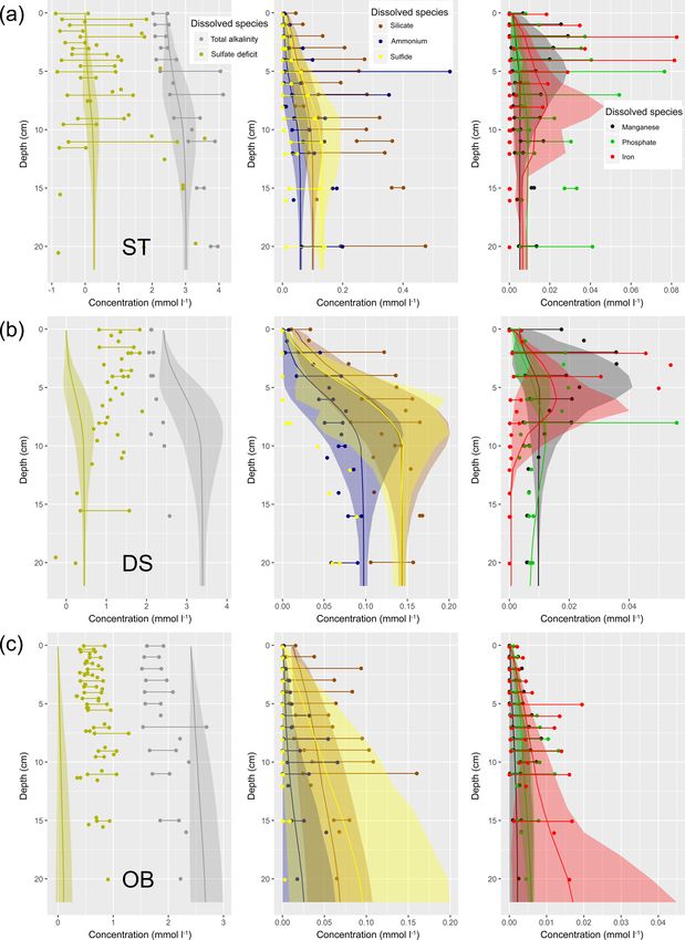
H. Radtke et al.: ERGOM with vertically resolved sediments 279
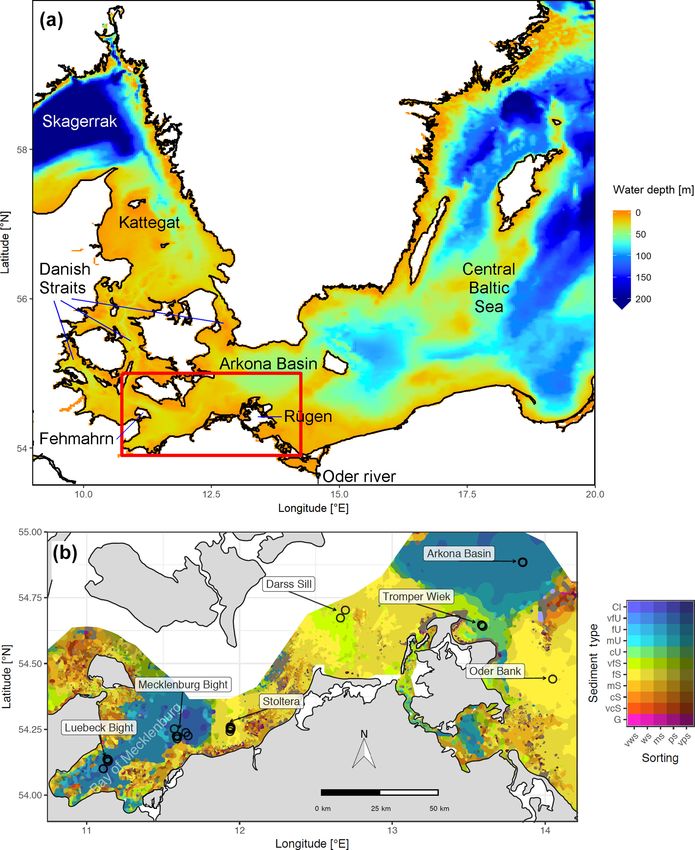
Figure 1. (a) Bathymetry of the western Baltic Sea and location of our area of interest. (b) The investigation area of the SECOS project. The
map shows granulometry, redrawn from Tauber (2012) and Lipka (2018), and the seven stations considered in this model study. Sediment
type: Cl – clay, vfU – very fine silt, fU – fine silt, mU – medium silt, cU – coarse silt, vfS – very fine sand, fS – fine sand, mS – medium
sand, cS – coarse sand, vcS – very coarse sand, G – gravel. Sorting: vws – very well sorted, ws – well sorted, ms – moderately sorted, ps –
poorly sorted, vps – very poorly sorted.
within a three-dimensional ecosystem model framework are model, so Sect. 2.2 describes how the physics affecting the
given. biogeochemical processes are prescribed. We then explain
the model compartments and state variables in Sect. 2.3. Be-
fore giving the full model equations in Sect. 2.5, we first ex-
2 Model description plain the vertical transport processes which occur in these
equations in Sect. 2.4.
In this section, we give a description of the combined The core of the model is obviously the biogeochemical
benthic–pelagic model. We start in Sect. 2.1 with a brief processes represented within it. Their description therefore
introduction to the two ancestor models it descended from. forms the major part of this paper. Biogeochemical processes
The model is a purely biogeochemical model, not a physical
www.geosci-model-dev.net/12/275/2019/ Geosci. Model Dev., 12, 275–320, 2019
280                                                                 H. Radtke et al.: ERGOM with vertically resolved sediments

in the water column are described in Sect. 2.6 and those in                  extensive literature survey (combined with model fitting
the sediment follow in Sect. 2.7. The carbonate system is                    to observations) allowed for the estimation of a large
the same in both compartments and is described separately                    quantity of model constants such as solubility products
in Sect. 2.8. Since most of the biogeochemical processes in-                 and half-saturation constants. These were later on inher-
cluded in our model are already contained in preceding mod-                  ited by several early diagenetic models, including the
els in exactly the same way, we decided to only give a qual-                 one presented in this article. These models solve the
itative description of them in the main text. The quantitative               diagenetic equations typically applied at a well-defined
details, including the values of the model constants we used,                single site as a one-dimensional set-up.
are presented in a separate, complete description in the Sup-                Like the present one, the model by Reed et al. (2011) is
plement. In contrast, we give a detailed and quantitative de-                a prognostic model and solves the time-dependent equa-
scription of the “new” processes in the main text, i.e. those                tions rather than making a steady-state assumption.
that are less common or those that differ from the ancestor
models, since we assume that this will be the most inter-              2.2   Physical parameters used in the model simulations
esting part for the majority of readers. The Supplement also
contains a table of the model constants and the sensitivities          Since our model is a purely biogeochemical model, it re-
of the model results to changes in the individual parameter            quires a physical environment in which it is embedded. In a
values.                                                                final, three-dimensional application, this will be a hydrody-
   The model description is completed by details on numeri-            namic host model, and the biogeochemical model described
cal aspects given in Sect. 2.9. Finally, in Sect. 2.10, we give a      in this communication will be coupled into it. Since we do an
short note on the procedure by which we automatically gen-             intermediate step first and run the model in one-dimensional
erate the model code from a formal description of the model            set-ups, we need to provide physical quantities as model in-
processes.                                                             put. The variables which influence the biogeochemical pro-
                                                                       cesses in the water column are
2.1   Ancestor models
                                                                         – temperature,
The combined benthic–pelagic model is based on two ances-
tors.                                                                    – salinity,

  – The water column part is based on ERGOM, an ecolog-                  – light intensity,
    ical model developed originally for the Baltic Sea (Neu-             – bottom shear stress and
    mann, 2000). It has been continuously developed since
    its first publication, and the latest improvements include           – vertical turbulent diffusivity.
    introducing refractory dissolved organic nitrogen (Neu-
    mann et al., 2015) and transparent exopolymers (Neu-               These are prescribed by forcing files1 which need to be pro-
    mann et al., 2017). From the start, ERGOM contained                vided in order to run the one-dimensional model. We obtain
    three functional groups of phytoplankton representing              these data from a three-dimensional model simulation of the
    large-cell (diatom) and small-cell (flagellate) primary            Baltic Sea ecosystem (Neumann et al., 2017). This simula-
    producers as well as diazotroph cyanobacteria and the              tion was performed using the Modular Ocean Model (MOM)
    ability to simulate hypoxic–anoxic conditions.                     version 5.1 (Griffies, 2018). The model had a horizontal res-
                                                                       olution of 3 nm and a vertical resolution of 2 m, covering
      ERGOM is typically used in a three-dimensional con-              the entire Baltic Sea. Open boundary conditions were ap-
      text as a part of marine ecosystem models. With some             plied in the Skagerrak at the transition to the North Sea.
      modifications, it has been applied for different ecosys-         The model was driven by atmospheric forcing data from the
      tems such as the North Sea (Maar et al., 2011) and               coastDat dataset (Weisse et al., 2009), which were extended
      the Benguela upwelling system (Schmidt and Eggert,               in time using data from the German Weather Service (Schulz
      2016). It is an intermediate-complexity model for the            and Schattler, 2014). The ERGOM ecosystem model, as de-
      lower trophic levels up to zooplankton and has been ap-          scribed in the previous section, was implemented in the phys-
      plied for a broad range of scientific questions.                 ical host model, so it produced a hindcast simulation of both
  – The sediment part is based on a model developed for                the physics and biogeochemistry of the Baltic Sea ecosystem.
    a study on the effect of seasonal hypoxia on sedimen-              We extracted model output from the simulated year 2015 at
    tary phosphorus accumulation in the Arkona Sea (Reed               the different locations as input for the 1-D model. Since we
    et al., 2011). This model is, as many others of its kind,             1 physics/temperature.txt,
    a descendant of the van Cappellen and Wang (1996)                  physics/salinity.txt, physics/light_at_top.txt,
    model, which focused on the sedimentary iron and man-              physics/bottom_stress.txt,
    ganese cycle and the mineralisation pathways of oxic               physics/diffusivity.txt, found in the subdirectories
    mineralisation, denitrification and sulfate reduction. An          stations/station_?? in the Supplement.

Geosci. Model Dev., 12, 275–320, 2019                                                     www.geosci-model-dev.net/12/275/2019/
H. Radtke et al.: ERGOM with vertically resolved sediments 281
run the 1-D model for a longer period, the physical forcing is
repeated every year.
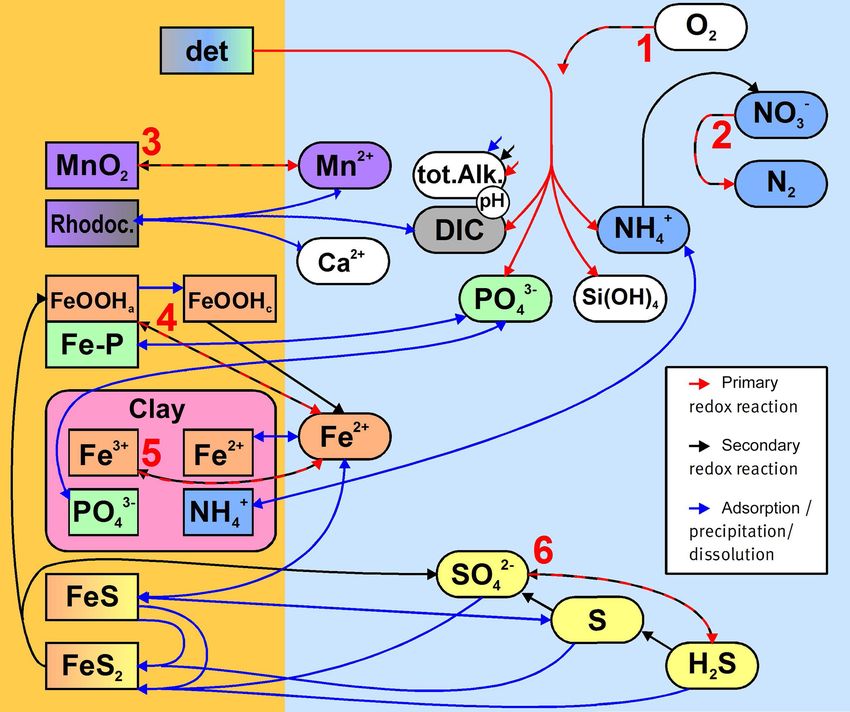
2.3 Model compartments and state variables
The one-dimensional model consists of four compartments
as shown schematically in Fig. 2:
1. the water column,
2. a fluff layer deposited on the sediment surface,
3. the sedimented solids and
Figure 2. Schematic view of the compartments and vertical ex-
4. the pore water between them. change processes in the model. Compartments: (I) water column,
(II) fluff layer, (III) pore water, (IV) solid sediment. Both the water
The water column and sediment are vertically resolved, column and sediment consist of several vertically stacked grid cells.
with the former in layers of 2 m depth such that their number Vertical transport processes: a – turbulent mixing, b – particle sink-
depends on the water depth of the specific site and the latter ing, c – sedimentation, d – resuspension, e – bioirrigation combined
in 22 layers increasing in depth from 1 mm at the sediment with molecular diffusion, f – bioturbation, g – sediment growth, h
surface to 2 cm at the bottom of the modelled sediment at – burial. Bioactive solid material is shown in orange, bioinert solid
22 cm of depth. These specific numbers are not intrinsic to material in grey and water in blue.
the model but can be changed in the input files2 . The current
choice of 22 cm for the sediment depth was made according
to the availability of pore water data. its constituents (OH− , H3 O+ , PO3−
4 ) which are actively pro-
The chosen vertical resolution must be seen as a compro- duced or consumed. The reasoning behind this is explained
mise between speed and accuracy. Especially for the 3-D ap- in Sect. 2.8.
plication, we want to keep the numerical effort of the calcula- The state variables will not be discussed one by one here,
tions as small as possible. A comparison to a run with double but rather in the section about the biogeochemical processes
resolution is shown in Appendix E, and it shows minor devi- (Sect. 2.6 and 2.7) where their role in the ecosystem will be
ations among the resolutions. explained.
Sediment porosity is prescribed3 and site specific. As a
simplifying assumption, accumulating organic material does
2.4 Transport processes
not change the porosity. Similarly, the amount of material
accumulated in the fluff layer does not change the remaining
volume in the bottom water cell. The processes which transport the tracers vertically are
The tracers (model state variables) present in each of the schematically shown in Fig. 2. Their detailed implementa-
compartments are listed in Table 1. All of the tracers have tion is discussed here.
a fixed stoichiometric composition, which is shown in Ap- Horizontal exchange (transport) is neglected in our one-
pendix A. When stoichiometric ratios change, such as during dimensional model. This is obviously an inadequate approx-
detritus decomposition, more than one tracer is needed. This imation for the water column processes, as we do not con-
means we can check mass conservation at the design time sider basins, but rather single stations, some of which are
of the model by formulating it in a process-based way as situated in proximity to river mouths where lateral transport
outlined in Radtke and Burchard (2015). To check this mass processes have a major impact (Schneider et al., 2010; Emeis
conservation, the chemical reaction equations need to be for- et al., 2002; Christiansen et al., 2002). We solve this issue
mulated in a complete way, which is why “virtual tracers” in the future application of the biogeochemical model in a
such as water may be included in the process formulation, three-dimensional model system (Cahill et al., 2019).
even if they do not occur as state variables in the model. In this model, we are not specifically interested in the wa-
Total alkalinity is a parameter describing the buffering ca- ter column as such but rather see it as being responsible for
pacity of a solution against adding acids; it describes the delivering the right amount of sedimenting detritus at the
amount of a strong acid that needs to be added to titrate it right time. To obtain this, we relax the wintertime nutrients
to a pH of 4.3. In our model, it is represented as a “com- in the surface layer to a realistic value. This may be seen as a
bined tracer”, which means that its rate of change depends on parameterisation of a lateral exchange process. In addition,
transport of fluff layer material away from or towards the
2 physics/cellheights.txt, modelled location is a lateral process included in the model.
physics/sed_cellheights.txt The physical processes which are explicitly included in our
3 physics/sed_inert_ratio.txt model are described here.
www.geosci-model-dev.net/12/275/2019/ Geosci. Model Dev., 12, 275–320, 2019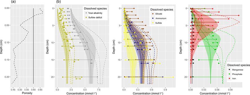
282                                                                                    H. Radtke et al.: ERGOM with vertically resolved sediments

Table 1. Tracers used in the ERGOM SED v1.0 model.

         Name                              W       F     S      P     Description                                           Unit
         t_lpp                              +                         large-cell phytoplankton                              mol kg−1   (N units)
         t_spp                              +                         small-cell phytoplankton                              mol kg−1   (N units)
         t_cya                              +                         diazotroph cyanobacteria                              mol kg−1   (N units)
         t_zoo                              +                         zooplankton                                           mol kg−1   (N units)
         t_det_?                            +                         detritus, N+C, fast decaying (1) to inert (6)         mol kg−1   (N units)
         t_detp_?                           +                         phosphate in detritus, fractions 1 to 6               mol kg−1   (N units)
         t_don                              +                         autochthonous dissolved organic nitrogen              mol kg−1
         t_poc                              +                         particulate organic carbon                            mol kg−1
         t_ihw                              +                         suspended iron hydroxide                              mol kg−1
         t_ipw                              +                         suspended phosphate bound to Fe (III)                 mol kg−1
         t_mow                              +                         suspended manganese oxide                             mol kg−1
         t_n2                               +                   +     dissolved molecular nitrogen                          mol kg−1
         t_o2                               +                   +     dissolved molecular oxygen                            mol kg−1
         t_dic                              +                   +     dissolved inorganic carbon                            mol kg−1
         t_alk                              +                   +     total alkalinity                                      mol kg−1
         t_nh4                              +                   +     ammonium                                              mol kg−1
         t_no3                              +                   +     nitrate                                               mol kg−1
         t_po4                              +                   +     phosphate                                             mol kg−1
         t_h2s                              +                   +     hydrogen sulfide                                      mol kg−1
         t_sul                              +                   +     elemental sulfur                                      mol kg−1
         t_so4                              +                   +     sulfate                                               mol kg−1
         t_fe2                              +                   +     ferrous iron                                          mol kg−1
         t_ca2                              +                   +     dissolved calcium                                     mol kg−1
         t_mn2                              +                   +     dissolved manganese (II)                              mol kg−1
         t_sil                              +                   +     silicate                                              mol kg−1
         t_ohm_quickdiff                    +                   +     OH− ions with realistically quick diffusion           mol kg−1
         t_ohm_slowdiff                     +                   +     OH− ions which move unrealistically slow with al-     mol kg−1
                                                                      kalinity
         t_sed_?                                   +     +            sedimentary detritus N+C, fractions 1 to 6            mol m−2 (N units)
         t_sedp_?                                  +     +            phosphate in sedimentary detritus, fractions 1 to 6   mol m−2 (N units)
         t_ihs                                     +     +            iron hydroxide in the sediment                        mol m−2
         t_ihc                                     +     +            iron hydroxide in the sediment – crystalline phase    mol m−2
         t_ips                                     +     +            iron-bound phosphate in the sediment                  mol m−2
         t_ims                                     +     +            iron monosulfide                                      mol m−2
         t_pyr                                     +     +            pyrite                                                mol m−2
         t_mos                                     +     +            manganese oxide in the sediments                      mol m−2
         t_rho                                     +     +            rhodochrosite                                         mol m−2
         t_i3i                                     +     +            potentially reducible Fe (III) in illite–             mol m−2
                                                                      montmorillonite mixed layer minerals
         t_iim                                     +     +            Fe (II) adsorbed to illite–montmorillonite mixed      mol m−2
                                                                      layer minerals
         t_pim                                     +     +            phosphate adsorbed to illite–montmorillonite mixed    mol m−2
                                                                      layer minerals
         t_aim                                     +     +            ammonium adsorbed to illite–montmorillonite           mol m−2
                                                                      mixed layer minerals
         h2o                                      virtual             water molecule
         h3oplus                                  virtual             hydronium ion
         ohminus                                  virtual             hydroxide ion
         i2i                                      virtual             structural Fe (II) in illite–montmorillonite mixed-
                                                                      layer minerals

       W: water column, F: fluff layer, S: solid sediment, P: pore water, ?: reactivity classes 1 to 6.

Geosci. Model Dev., 12, 275–320, 2019                                                                      www.geosci-model-dev.net/12/275/2019/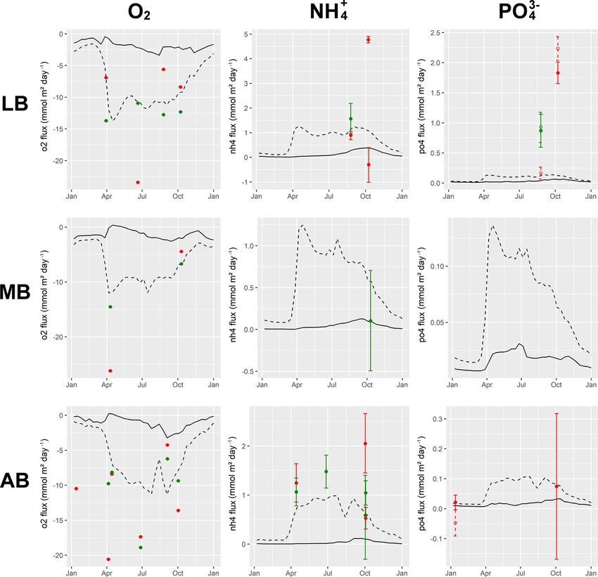
H. Radtke et al.: ERGOM with vertically resolved sediments                                                                            283

2.4.1   Turbulent mixing                                            transport represents winnowing of sediments (Bale and Mor-
                                                                    ris, 1998).
Vertical exchange due to turbulent mixing in the water col-
umn is prescribed externally4 by a turbulent diffusivity. In        2.4.4   Bioerosion
our case, it is taken from a three-dimensional MOM5 model
run (Neumann et al., 2017). In this model set-up, turbulent         In environments with oxic bottom waters, we assume that in
vertical mixing is estimated by the KPP turbulence scheme           addition to waves and currents, macrofaunal animals or dem-
(K profile parameterisation; Large et al., 1994), which con-        ersal fish can resuspend organic material from the fluff layer
siders both local mixing and, in the case of unstable stratifi-     by active movements (Graf and Rosenberg, 1997). Therefore,
cation, (non-local) convection. We only take into account the       under oxic conditions, we assume that rbiores = 3 % day−1
local part of the mixing and apply it to all tracers in the water   of the fluff material is resuspended independently from the
column.                                                             shear stress conditions. This number was estimated from
                                                                    the calibration of a three-dimensional Baltic Sea ecosystem
2.4.2   Particle sinking                                            model (Neumann and Schernewski, 2008) in which the pro-
                                                                    cess proved to be critical for transporting organic matter to
In our model, suspended particulate matter sinks at a constant      the deep basins below a depth of approx. 60 m. In these
rate through the water column. We choose 4.5 m day−1 for            depths, a resuspension due to wave-induced shear stress is
detritus, 1 m day−1 for manganese and iron oxides, including        no longer possible.
the phosphate adsorbed by them, and 0.5 m day−1 for large-
cell phytoplankton and particulate organic carbon. In con-          2.4.5   Bioturbation
trast, cyanobacteria are not sinking but, due to their positive
buoyancy, they show an upward movement of 0.1 m day−1 .             Bioturbation describes the movement and mixing of particles
In reality, the sinking rate differs among individual particles;    inside the sediment caused by the zoobenthos.5 In fact, it is
the currently chosen average values are a result of fitting the     difficult to discriminate what causes the vertical mixing of
previous ERGOM model with the simplified sediment repre-            particles; physical effects like bottom shear may also have
sentation to observations.                                          the same effect. We therefore include them in our “bioturba-
                                                                    tion” process.
2.4.3   Sedimentation and resuspension                                 We consider bioturbation to act as a vertical diffusiv-
                                                                    ity DB,solids (z) on the concentrations of the different solid
Shear stress at the bottom determines whether erosion or sed-       species in the sediment. This implies that we exclude non-
imentation takes place. We apply the combined shear stress          local mixing processes, even if they may be important in na-
of currents and waves calculated by the same MOM5 model             ture (Soetaert et al., 1996b), and try to represent them by
as the turbulent mixing. If this shear stress τ is below a crit-    local mixing. We only take intraphase mixing into account,
ical value of τc = 0.016 N m−2 (Christiansen et al., 2002),         which means we assume that the porosity 8(z) remains con-
the sinking suspended matter accumulates in the fluff layer         stant over time.
compartment. If it is exceeded, the fluff layer material is re-        The diffusivity DB,solids (z) is also applied to describe the
suspended into the lowest water cell at a constant relative rate    transport between the uppermost sediment layer and the fluff,
rero = 6 day−1 .                                                    which is caused by benthic organisms. In reality, the fluff
   In our model, no material will ever be resuspended from          layer may strongly differ in its compaction (porosity) de-
the sediment itself, which starts below the fluff layer. This       pending on the turbulence conditions. However, we assume
means that our model is incapable of realistically capturing        it to be perfectly compacted (φ = 0) to be able to apply the
extreme events like storms or bottom trawling which winnow          above equation to describe the exchange process and there-
the upper layers of the sediment, removing organic material,        fore assume a thickness of 3 mm. This is not a physical as-
which has a lower sinking velocity, by separating it from the       sumption but rather a numerical trick which we use to trans-
heavier mineral components (Bale and Morris, 1998). It also         port the fluff material into the sediments. In reality, the fluff
neglects a washout, which is the removal of organic matter          layer may be up to a few centimetres thick, and the incor-
from the sediment pores by advective transport of pore water        poration of organic matter is done by macrofaunal activities
by strong bottom currents (Rusch et al., 2001). In our model,       (e.g. van de Bund et al., 2001).
sediment reworking by currents and waves is not explicitly             The value 3 mm describes a volume estimate of SPM (sus-
represented, but rather parameterised together with the bio-        pended particulate matter) taken from this region: typical
turbation process. This process allows for a bi-directional         SPM concentrations in the lowermost 40 cm of the water col-
exchange of particulate material between the sediment and              5 While bioturbation in reality causes both a transport of solids
the fluff layer; see Sect. 2.4.5. The upward component of the       and solutes, we use the term “bioturbation” in the model to describe
                                                                    the transport of solids only, while the transport of solutes is done by
   4 physics/diffusivity.txt                                        the “bioirrigation” process.

www.geosci-model-dev.net/12/275/2019/                                                      Geosci. Model Dev., 12, 275–320, 2019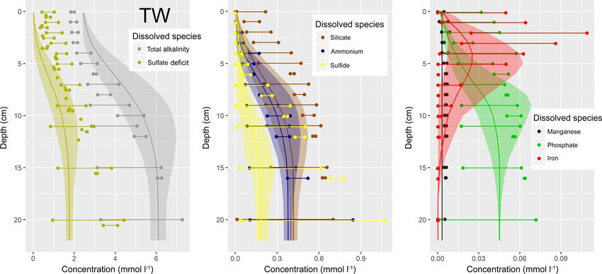
284 H. Radtke et al.: ERGOM with vertically resolved sediments
umn are about 8 mg L−1 higher compared to the value 5 m the effect of hydrodynamic tortuosity θ . This describes the
above the sea floor (Christiansen et al., 2002). As the den- effect that the solutes need to travel a longer path as the di-
sity of these particles is just slightly higher than that of the rect way may be obstructed by solid particles. It is estimated
surrounding water, we can estimate their volume at approx- from porosity by θ 2 = 1 − 2.02 ln(φ) (Boudreau, 1997).
imately 3 L m−2 , which gives 3 mm of height if perfectly A diffusive exchange between the pore water and the over-
compacted. We see this explicit treatment of the fluff layer as lying bottom water is controlled by the thickness of a diffu-
a major advantage compared to the deposition of sinking par- sive boundary layer. While in reality this relates to the vis-
ticles directly into the surface sediments. We regard it as es- cous sublayer thickness and is therefore inversely related to
sential for the application of the model in a three-dimensional the velocity of the bottom water (Boudreau, 1997), for sim-
setting. plicity we assume a constant diffusive boundary layer thick-
The vertical structure of bioturbation intensity, ness of 3 mm.
DB,solids (z), is parameterised vertically as follows. In reality, the diffusive boundary layer thickness is on the
order of 1 mm at low-bottom-shear situations and becomes
DB,solids (z) = (1)
even shallower if the bottom shear increases (e.g. Gundersen
DB,solids,max for z < zfull and Jorgensen, 1990). We choose a larger value because we
z − zfull need to account for the transport through the fluff layer as
DB,solids,max exp − for zfull < z < zmax
zdecay well. A future model version might include a dependence of
0 for zmax < z
this parameter on the bottom shear stress.
In the uppermost part of the sediment, we assume a con- Molecular diffusivities for the different solute species are
stant bioturbation rate. Below that, it decays exponentially calculated from water viscosity following Boudreau (1997).
with depth until it reaches a maximum depth, which may The water viscosity is determined from salinity and tem-
be below the bottom of our model. So, we externally pre- perature (assumed to be identical to that in the bottom wa-
scribe (a) the maximum mixing intensity6 and (b) three ter cell). A problem occurs with the combined tracers DIC
length scales describing the vertical structure of bioturba- and total alkalinity, as they do not represent a specific ion
tion7 , which are the depth down to which the maximum mix- but rather a set of different species with different molecu-
ing rate is applied (zfull ), the length scale of the exponential lar diffusivities. For simplicity, we approximate DIC diffu-
decay of the mixing rate below this depth (zdecay ) and the sivity to be that of the HCO− 3 ion, the most common one
maximum depth of mixing (zmax ). at the pH values we expect. For total alkalinity, we take a
The present formulation of the model has no explicit de- two-step approach: in the first step, we also take the diffu-
pendence of bioturbation depth on the availability of oxi- sivity of the HCO− 3 ion. But this is an underestimate, es-
dants, i.e. bioturbation will take place in oxic as well as in pecially for the OH− ions, which increase in concentration
sulfidic environments; adding this dependence should be es- as the solution becomes alkaline. To take their higher dif-
sential if the model is applied to sulfidic areas. fusivity into account, we introduce two additional tracers,
t_ohm_slowdiff and t_ohm_quickdiff. Before the
2.4.6 Bioirrigation molecular diffusion is applied during a model time step, they
are both set equal to the OH− concentrations. During the dif-
Bioirrigation describes the mixing of solutes within the pore fusion time step, the former diffuses with the reduced HCO− 3
water and the exchange with the bottom water. We describe diffusion rate, the latter with the OH− diffusivity. So after-
it as a mixing intensity DB,liquids (z). The vertical profile of wards, total alkalinity is corrected by adding the difference of
bioirrigation intensity is assumed identical to that of biotur- the two, t_ohm_quickdiff-t_ohm_slowdiff. This
bation. The maximum bioirrigation rate is assumed constant results in a smoothed alkalinity profile.
in time and prescribed externally8 .
2.4.8 Sediment accumulation
2.4.7 Molecular diffusion
In nature, sediments grow upwards as new particulate matter
Molecular diffusion in the sediment can be described by the is deposited onto them. In our model, this process is taken
equation into account, but represented as the downward advection of
material in the sediment. So, our coordinate system moves
∂ ∂ φ(z) ∂c(z, t)
φ(z) c(z, t) = D0 (z) (2) upward with the sediment surface. We assume that the sedi-
∂t ∂z θ (z)2 ∂z
ment growth is supplied by terrigenous, bioinert material and
(Boudreau, 1997). Here, D0 describes the molecular diffusiv- prescribe9 a growth rate from the literature for the mud sta-
ity in a particle-free solution, which is effectively reduced by tions only (Table 7). We do not assume sediment growth for
6 physics/sed_diffusivity_solids.txt the sand and silt stations.
7 physics/sed_depth_bioturbation.txt
8 physics/sed_diffusivity_porewater.txt 9 physics/sed_inert_deposition.txt
Geosci. Model Dev., 12, 275–320, 2019 www.geosci-model-dev.net/12/275/2019/H. Radtke et al.: ERGOM with vertically resolved sediments 285
We use a simple Euler-forward advection to move the ma- ∂ wat ∂ ∂
= −w c (z, t) + D wat (z, t) cwat (z, t)
terial from each grid cell into the cell below. Material leaving ∂z ∂z ∂z
the model through the lower boundary is lost. Except for or- wat
+ qc (z, t), (4)
ganic carbon, we assume that a part of it is mineralised, as
will be explained in Sect. 2.7.1. In the top cell, new organic where qcwat (z, t) describes the biogeochemical sources minus
material from the fluff layer enters by sediment growth. sinks of the considered state variable.
The equations in the sediment are different because we
2.4.9 Parameterisation of lateral transport need to take porosity into account and treat dissolved trac-
ers (in the pore water) and solid tracers differently. For the
The Baltic Sea sediments can be classified as accumulation, pore water tracers, the upward flux is given by
transport and erosion bottoms (Jonsson et al., 1990). The lat-
eral transport of matter is characterised by the advection of pw ∂ pw
Fz (z, t) = −φ(z) · D pw (z, t) c (z, t), (5)
fluff layer material from the transport and erosion bottoms in ∂z
the shallower areas to the accumulation bottoms in the deep where φ(z) is the porosity of the sediment (the ratio between
basins (Christiansen et al., 2002). As this process is not rep- pore water volume and total volume), which we assume as
resented in our 1-D model set-ups, we need to parameterise constant in time. The concentration cpw (z, t) relates to the
it. pore water volume only. The effective diffusivity D pw is the
For the sandy and silty sediments, we assume transport sum of two contributions, the effective molecular diffusivity
away from the site. This is described by a constant removal D0
and the effective (bio)irrigation diffusivity DB,liquids (z).
θ2
rate for all material deposited in the fluff layer. For the mud The advection–diffusion equation is then given by
stations, we assume transport of organic material towards the
site. This is described by a constant input of detritus. Our ∂ pw ∂ pw ∂ pw
φ(z) c (z, t) = φ(z) · D (z, t) c (z, t)
model contains six detritus classes which degrade at different ∂t ∂z ∂z
rates, as will be explained later in Sect. 2.6.4. We assume that pw
+ qc (z, t), (6)
the quickest-degradable part of the detritus is already miner-
alised in the shallow coastal areas before its lateral migration which is a well-known early diagenetic equation (Boudreau,
to the mud stations and therefore exclude the first two classes 1997). For the solid-state tracers, their concentration
from this artificial input. csed (z, t) relates to the volume of the solids only, and the flux
In the 3-D version of the model, these processes are no is given by
longer required, as the material is dynamically removed from
the shallow sites and transported to deeper ones by advection. Fzsed (z, t) = (1 − φ(z))w(z)csed (z, t) − (1 − φ(z))
∂
2.5 Model equations · D sed (z, t) csed (z, t), (7)
∂z
2.5.1 Equations of motion where w(z) is the velocity for virtual vertical downward
transport. It results from sediment growth due to the depo-
In this subsection, we will describe the equations of motion sition of particulate material, but as we keep the sediment–
solved by the model. The equations in the water column can water interface at a constant position in our model, we need
be derived from the assumption that the vertical (upward) to describe the increasing depth in which we find individual
flux of a tracer can be described by an advective and a diffu- sediment particles as downward advection. Volume conser-
sive flux, which follows Fick’s law: vation of the particulate material requires that we write w(z)
∂ wat as
Fzwat (z, t) = w · cwat (z, t) − D wat (z, t) c (z, t), (3) w0
∂z w(z) = (8)
1 − φ(z)
where cwat (z, t) denotes the tracer concentration and D wat
is the turbulent diffusivity given as external forcing10 . For such that the vertical velocity gets smaller in depths at which
particulate matter, the constant w describes its vertical ve- the sediment is more compacted, and w0 describes a the-
locity relative to the water, which is negative if the particles oretical velocity which would occur at perfect compaction
are sinking. For dissolved tracers, w is set to zero. We fur- (φ = 0)11 . The advection–diffusion equation then reads
ther assume that the water itself does not move vertically. In
this case, conservation of mass yields an advection–diffusion ∂ sed ∂ sed ∂
(1 − φ(z)) c (z, t) = −w0 c (z, t) + (1 − φ(z))
equation: ∂t ∂z ∂z
∂ wat ∂ ∂
c (z, t) = − Fzwat (z, t) + qcwat (z, t) · DB,solids (z) csed (z, t) + qcsed (z, t). (9)
∂t ∂z ∂z
10 physics/diffusivity.txt 11 physics/sed_inert_deposition.txt
www.geosci-model-dev.net/12/275/2019/ Geosci. Model Dev., 12, 275–320, 2019286 H. Radtke et al.: ERGOM with vertically resolved sediments
Practically, we do not store the concentration csed (z, t) At the sea surface, we apply a zero-flux condition, both for
(mol m−3 ) as a state variable but rather the quantity of the dissolved and particulate state variables:
tracer per area in a specific layer, C sed (k, t) (mol m−2 ), where
k is a vertical index. The transformation is straightforward: Fzwat (zsurf , t) = 0. (14)
top,k
zZ An exception is only made for tracers which are modified by
sed sed gas exchange with the atmosphere, e.g. oxygen.
C (k, t) = (1 − φ(z)) c (z, t)dz. (10)
Now the boundary conditions for the particulate state vari-
zbot,k ables are different. The reason is that the water column and
the sediment do not directly interact, but we consider the fluff
For particulate tracers, we also consider storage in the fluff
layer as an intermediate layer between the two. Particulate
layer, C fluff (t), which is measured in mol m−2 . The equation
material which sinks to the bottom is deposited in the fluff
for C fluff (t) is derived in the following subsection.
layer, from which it is incorporated into the sediments.
At the bottom of the water column, there can be two pos-
2.5.2 Boundary conditions
sible situations.
Boundary conditions are required for the partial differential – If the bottom shear stress is lower than the critical shear
equations given above. We give two boundary conditions for stress, we assume a deposition of particulate material.
the water column concentrations: one at the sea surface, zsurf , This sinking material (w < 0) vanishes from the water
and one at the sediment–water interface, z0 . We also give two column because of sedimentation. It appears in the fluff
boundary conditions for the sediment concentrations: one at layer.
the sediment–water interface, z0 , and one at the lower model
boundary, zbot . We start describing the boundary conditions – If the bottom shear stress exceeds the critical shear
from bottom to top for the dissolved tracers and then continue stress, particulate material from the fluff layer is eroded
describing them from top to bottom for the particulate and and enters the water column.
solid-phase state variables.
The pore water tracers have a zero-flux boundary condi- In both cases, we additionally consider the bioresuspension
tion at the bottom of the model: process which was described above in Sect. 2.4.4. We can
therefore formulate the boundary condition for particulate
pw material as
Fz (zbot , t) = 0. (11)
An exception to the zero-flux boundary is the parameteri- Fzwat (z0 , t) = (15)
wat fluff
sation of sulfide production in the deep, which will be dis- min(w, 0) · c (z0 , t) + rbiores (t) · C (t) for τ (t) ≤ τc
.
cussed later. rero · C fluff (t) + rbiores (t) · C fluff (t) for τ (t) > τc
At the sediment–water interface, we assume that the dis-
solved tracers are exchanged between pore water and the wa- The fluff interacts with the surface sediment layer in two
ter column via a diffusive boundary layer of a depth 1zbbl . ways. Firstly, sediment growth means an incorporation of
So, our upper boundary condition for the pore water tracers fluff layer material into the surface sediments. Secondly, bio-
is given by turbation, which is considered diffusion–analogue mixing,
leads to an exchange of particulate material between the fluff
pw
Fz (z0 , t) = −φ(z0 ) layer and surface sediment. So, the boundary condition for
solids at the sediment surface is given by
cwat (z0 , t) − cpw (z0 , t)
· D pw (z0 , t) . (12)
1zbbl C fluff (t)
Fzsed (z0 , t) = w0 − (1 − φ(z0 ))
1zfluff
This flux can be directed into or out of the sediment, depend-
C fluff (t)
ing on where the concentration is larger. sed 1zfluff − csed (z0 , t)
To satisfy mass conservation, the vertical flux applied as ·D (z0 , t) . (16)
1zfluff
the lower boundary condition for the dissolved species con-
centrations in the water column depends on the upward flux Here, 1zfluff represents a virtual thickness of the fluff layer
from the sediment: assuming it was perfectly compacted; see the discussion in
Sect. 2.4.5. In this way, the benthofaunal processes of incor-
pw
Fzwat (z0 , t) = Fz (z0 , t) + Q
efluff
c (t). (13) porating fluff layer material into the surface sediments can be
simply described as a diffusion–analogue flux of particulates.
The additional term Qefluff (t) represents the sources minus The opposite processes which cause removal of fine-grained
sinks of the dissolved state variable, which are caused by material from the sediments, winnowing or washout, can be
biogeochemical transformations of the fluff layer material. described in the same way as a diffusion process, in this case
Geosci. Model Dev., 12, 275–320, 2019 www.geosci-model-dev.net/12/275/2019/H. Radtke et al.: ERGOM with vertically resolved sediments 287
upward. This occurs in the model, especially when the fluff the result of a cellular carbon overflow whenever nutrient ac-
layer material is resuspended during periods of high bottom quisition limits biomass production but not photosynthesis.
shear and the concentration C fluff (t) is correspondingly low. These transparent exopolymers are included in our model,
The concentration change in the fluff layer is then defined and they are assumed to have a constant sinking velocity.
by mass conservation and is simply given by
2.6.2 Phytoplankton respiration and mortality
∂ fluff
C (t) = Fzsed (z0 , t) − Fzwat (z0 , t) + Qfluff
c (t) (17)
∂t We assume a constant respiration of phytoplankton which
pw is proportional to its biomass. As the model maintains the
for all particulate state variables. Here, describes the
Qc (t)
Redfield ratio, the degradation of biomass (catabolism) goes
sources minus sinks term from the biogeochemical transfor-
along with the excretion of ammonium and phosphate. This
mations of the considered state variable.
simplified description of phytoplankton growth does not de-
Finally, the burial of particulate material at the lower
scribe day–night metabolism or temperature dependence. A
model boundary can be described by the following bound-
small fraction of the nitrogen is released as dissolved organic
ary condition:
nitrogen (DON). In the model, this represents the DON frac-
Fzsed (zbot , t) = w0 csed (zbot , t). (18) tion which is less utilisable by phytoplankton, while the frac-
tion with high bioavailability is considered to be part of the
So, we assume the particulate material to be buried forever ammonium state variable.
when it leaves the model domain. An exception, as men- Due to simplification, in our model phytoplankton expe-
tioned before, is the parameterisation of deep sulfide forma- riences a constant background mortality, although we know
tion, which is described in Sect. 2.7. this is far away from reality in which it is species specific and
depends on abiotic (e.g. nutrient, light, etc.) and biotic con-
2.6 Biogeochemical processes in the water column ditions. An additional mortality is generated by the grazing
of zooplankton as described next.
In this section, we describe the biogeochemical processes
acting in the water column. These are mostly identical to 2.6.3 Zooplankton processes
previously published ERGOM versions (e.g. Neumann and
Schernewski, 2008; Neumann et al., 2015), which contained Zooplankton is only represented as one bulk state variable.
a more simple, vertically integrated sediment model. As in It grows by assimilating any type of phytoplankton; how-
the previous section, we provide a quantitative description ever, it has a smaller food preference for the cyanobacte-
including the model constants in the Supplement. ria class compared to the other classes. The uptake becomes
A reaction network table giving the reaction equations, in- limited by a Michaelis–Menten function if the zooplankton’s
cluding their stoichiometric coefficients, is given in Table 2. food approaches a saturation concentration. Feeding can only
take place in oxic waters and is temperature dependent. It
2.6.1 Primary production and phytoplankton growth shows a maximum at an optimum temperature and a double-
exponential decrease when this temperature is exceeded.
There are three classes of phytoplankton in the model, rep-
Both zooplankton respiration and mortality represent a
resenting large-cell and small-cell microalgae as well as di-
closure term for the model. They are meant to include the
azotroph cyanobacteria. Their growth is determined by a
respiration and mortality of the higher trophic levels (fish)
class-specific maximum growth rate, but contains two limit-
which feed on zooplankton, and therefore we use a quadratic
ing factors for nutrients and light. The light limitation is a sat-
closure. Mortality is additionally enhanced under anoxic
uration function with optimal growth at a class-specific opti-
conditions, which do not occur in our study area.
mum level or at 50 % of the surface radiation. The shortwave
light flux at the surface is taken from a dynamically down-
2.6.4 Mineralisation processes
scaled ERA40 atmospheric forcing (Uppala et al., 2005) us-
ing the regional Rossby Centre Atmosphere model (RCA). The description of detritus12 differs from the previous ER-
Nutrient limitation is a quadratic Michaelis–Menten term GOM versions. We have split the detritus into six classes, de-
for DIN (nitrate + ammonium) or phosphate, depending on pending on its degradability. This degradability is described
which one is limiting, based on Redfield stoichiometry. Dia- as a decay rate constant, which ranges from 0.065 day−1 for
zotroph cyanobacteria are only limited by phosphate and not the first class to 1.6×10⁻⁵ day−1 for the fifth class, while the
by DIN, but they are only allowed to grow in a specific salin- last one is assumed to be completely bioinert. This type of
ity range. Cyanobacteria and small-cell algae also require a
minimum temperature to grow (Wasmund, 1997; Andersson 12 Throughout the paper, we use the term “detritus” in its biolog-
et al., 1994). ical meaning; here, it describes dead particulate organic material
However, according to Engel (2002), although nutrients only, as opposed to its use in geology, where the term includes de-
are limiting an enhanced polysaccharide exudation could be posited mineral particles.
www.geosci-model-dev.net/12/275/2019/ Geosci. Model Dev., 12, 275–320, 2019You can also read