Queensland's Integrated Marine Observing System (Q-IMOS) Node Science and Implementation Plan 2015-25 - Australian Integrated Marine ...
←
→
Page content transcription
If your browser does not render page correctly, please read the page content below
Queensland’s Integrated
 Marine Observing System
      (Q-IMOS) Node
Science and Implementation
            Plan
          2015-25

     IMOS is a national collaborative research infrastructure, supported
      by Australian Government. It is led by University of Tasmania in
         partnership with the Australian marine & climate science
                                community.

                                                                           1
IMOS Node Queensland’s Integrated Marine Observing System
Lead Institution Australian Institute of Marine Science
Name: Richard Brinkman
Affiliation: Australian Institute of Marine Science
Node Leader(s)
Address: PMB 3, Townsville MC, QLD 4810
Phone: 07 4753 444
Email: r.brinkman@aims.gov.au
Name: Russ Babcock
Affiliation: CSIRO Marine and Atmospheric Research
Deputy Node Leader(s)
Address: PO Box 120, Cleveland, QLD 4163
Phone: 07 3826 7184
Email: russ.babcock@csiro.au
Commonwealth Scientific and Industrial Research Organisation
(CSIRO)
Griffith University
Healthy Waterways Partnership
Queensland Department of Environment and Heritage Protection
(QDEHP)
Queensland Department of Agriculture, Fisheries and Forestry
(QDAFF)
Collaborating Institutions
Queensland Department of Science, Information Technology,
Innovation and the Arts (QDSITIA)
Tropical Marine Network covering island research stations operated
by
Australian Museum (Lizard)
James Cook University (Orpheus)
University of Queensland (Heron)
University of Sydney (One Tree)
Lead authors: Peter Doherty, Russ Babcock, Anthony Richardson
Contributing authors: Richard Brinkman, Craig Steinberg, Scott Bainbridge, Janice Lough,
Miles Furnas, David McKinnon
Edited by: Peter Doherty, Katy Hill, Shavawn Donoghue, Richard Brinkman
Date: 27 May 2013
2
Table of Contents
Table of Contents .................................................................................................................................... 3
1      Executive Summary ......................................................................................................................... 5
2      Socio-economic context .................................................................................................................. 7
    2.1       Great Barrier Reef ................................................................................................................... 7
    2.2       South East Queensland............................................................................................................ 8
    2.3       Torres Strait and Gulf of Carpentaria...................................................................................... 8
    2.4       The value of a marine observing system in Queensland ......................................................... 9
3      Scientific Background, by Major Research Theme........................................................................ 17
    3.1       Multi-decadal ocean change.................................................................................................. 17
       3.1.1          The global energy balance (temperature) and sea level budget .................................... 17
       3.1.2          The global ocean circulation ......................................................................................... 20
       3.1.3          The global hydrological cycle (salinity) ....................................................................... 21
       3.1.4          The global carbon cycle (Inventory, air sea fluxes, physical controls) ......................... 21
       3.1.5          Science Questions ......................................................................................................... 24
       3.1.6          Notable gaps and future priorities ................................................................................. 24
    3.2       Climate variability and weather extremes ............................................................................. 24
       3.2.1          Interannual Climate Variability .................................................................................... 24
       3.2.2          Intra-seasonal variability and severe weather ............................................................... 30
       3.2.3          Science Questions ......................................................................................................... 39
       3.2.4          Notable gaps and future priorities ................................................................................. 39
    3.3       Major boundary currents and inter-basin flows .................................................................... 40
       3.3.1          South Equatorial Current .............................................................................................. 40
       3.3.2          East Australian Current (EAC) system ......................................................................... 41
       3.3.3          Gulf of Papua Current ................................................................................................... 44
       3.3.4          Science questions .......................................................................................................... 45
       3.3.5          Notable gaps and future priorities ................................................................................. 46
    3.4       Continental Shelf and Coastal Processes .............................................................................. 47
       3.4.1          Boundary current eddy –shelf interactions ................................................................... 47
       3.4.2          Upwelling and downwelling ......................................................................................... 47
       3.4.3          Shelf Currents ............................................................................................................... 53
       3.4.4          Wave climate, including internal and coastally trapped waves. ................................... 56
       3.4.5          Science questions .......................................................................................................... 57
       3.4.6          Notable gaps and future priorities ................................................................................. 58
    3.5       Ecosystem Responses ........................................................................................................... 59

                                                                                                                                                      3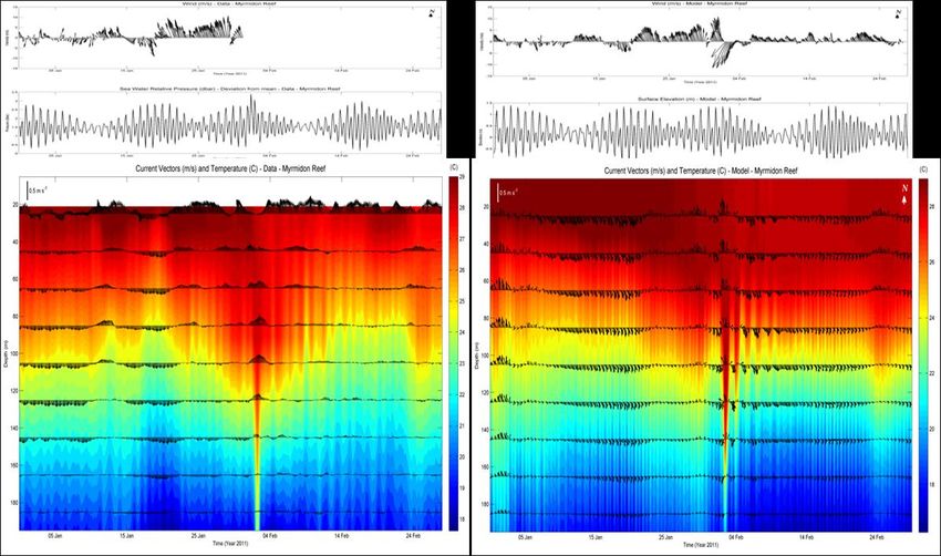
3.5.1         Temperature .................................................................................................................. 59
      3.5.2         Ocean Chemistry – Nutrients ........................................................................................ 60
      3.5.3         Ocean Chemistry – Carbon and acidification ............................................................... 62
      3.5.4         Plankton ........................................................................................................................ 64
      3.5.5         Mid Trophic Levels (Nekton) ....................................................................................... 65
      3.5.6         Top Predators ................................................................................................................ 67
      3.5.7         Benthos ......................................................................................................................... 69
      3.5.8         Science questions .......................................................................................................... 69
      3.5.9         Notable gaps and future priorities ................................................................................. 70
4     How will the data provided by IMOS be taken up and used?....................................................... 71
    4.1      Existing requirements by Node partners ............................................................................... 76
    4.2      Partnership opportunities ...................................................................................................... 77
    4.3      Enhanced research training ................................................................................................... 77
5     Regional, national and global impacts of IMOS observations ...................................................... 78
    5.1      Regional impacts ................................................................................................................... 78
    5.2      National impacts ................................................................................................................... 79
    5.3      International impacts ............................................................................................................. 80
6     Governance, structure and funding .............................................................................................. 82
7     References .................................................................................................................................... 83

                                                                                                                                                      4
1      Executive Summary

In 2006, the Integrated Marine Observing System (IMOS), the Queensland Government, and the
Collaborating Partners committed over $14M to the creation of a Great Barrier Reef Ocean
Observing System (GBROOS) as the Queensland Node of IMOS. In 2007, the first data streams from
moored instruments were placed in the national archive, now known as the Australian Ocean Data
Network (AODN), and the entire allocated infrastructure was in place by 2009.

In 2009, the IMOS Board enhanced GBROOS with several new capabilities (ocean gliders, acoustic
receivers, pCO2/pH sensors) and funded a National Reference Station (NRS) in South East
Queensland (Figure 1). Following this expansion beyond the Great Barrier Reef Marine Park, the
Node was rebranded as Queensland’s Integrated Marine Observing System (Q-IMOS).

    Figure 1. Map of Queensland showing three geographic regions referenced in this Plan. The
    transitions are Cape York (north) and Fraser Island (south).

The Q-IMOS Node Science and implementation Plan (NSIP) is based on understanding the impacts of
ocean variability in the Coral Sea upon the condition and productivity of shelf ecosystems along the
east coast of Queensland, with a current focus on the section of the continental shelf influenced by
the southerly-flowing East Australian Current (EAC). This region includes the southern half of the
iconic Great Barrier Reef (GBR), the majority of Queensland’s commercial fisheries production, and
the great majority of the State’s coastal population. It is also contiguous with the NSW-IMOS

                                                                                                   5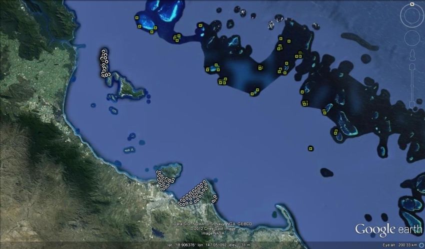
observing region providing a synoptic view of Australia’s most important coastal boundary current
(the EAC).

Currently, Q-IMOS activities are constrained to these priorities but this leaves more than half of the
Queensland coast without any in-situ marine observations. This gap includes the northern GBR
(influenced by the northerly-flowing Gulf of Papua Current), the Torres Strait, and the Gulf of
Carpentaria (Figure 1). Thus a major challenge for the Node in the life of this Plan (2015-2025) is
finding the resources to plug these critical knowledge gaps.

                                                                                         January 2014

                                                                                                         6
2 Socio-economic context

Many of Australia’s most precious natural assets are located in Queensland. These include a wide
range of commodity resources as well as the iconic GBR, which is one of the world’s most important
biodiversity assets. Major economic activities such as mining, agriculture, shipping, fishing, urban
development, tourism and recreation converge at the Queensland coast and their cumulative
impacts are major drivers of ecosystem status and trend. The legacy of past development and
population growth is coastal and marine areas with degraded water quality, and losses of habitat
and biodiversity. The rapid pace of projected development will produce ever greater cumulative
risks over the next decade, requiring nimble adaptive management and evidence-based decisions.

2.1 Great Barrier Reef
The GBR is the World’s largest reef archipelago stretching >2,000 km from Cape York to Lady Elliot
Island, which lies just 80 km north of the northern tip of Fraser Island. Today, the GBR is a multiple-
use marine park generating more than $5 billion of annual economic activity and supporting around
70,000 jobs (GBR Outlook Report 2009). The Great Barrier Reef Marine Park (GBRMP) is also a World
Heritage Area recognized internationally for its Outstanding Universal Value, which is today being
threatened by the cumulative impacts of multiple human uses and ongoing climate change.

In 2003, the Australian and Queensland Governments recognised that broad-scale agriculture in the
coastal catchments was having a deleterious impact on marine receiving waters in some sections of
the Park due to the export of unnaturally high loads of sediments, nutrients, and pesticides in river
run-off. In response, both governments committed to halt and reverse the decline of water quality
entering the GBR Lagoon through a decadal program (Reef Plan) that is based on changing land
management practices. Following a mid-term review and a Scientific Consensus raising concern
about the level of threat, the two governments committed $375 million to support Reef Plan actions
(2009-13). In 2013, after an update of the Scientific Consensus (Brodie et al. 2013b) and review of
the Program showing some load reductions, Reef Plan was extended for a further five years (2013-
18) with a similar level of investment and an aspirational target that “water quality should have no
detrimental impact on GBR ecosystems by 2020”.

Other pressures within the GBRMP (e.g. marine tourism, commercial and recreational fishing) are
managed by a variety of regulatory apparatus including the GBR Zoning Plan that determines
appropriate use. In 2004, a significant rezoning of the Park resulted in a third of 70 recognised
bioregions being reserved in ‘no take ‘zones. As part of the re-zoning, the Great Barrier Reef Marine
Park Authority (GBRMPA) is required to inform the Australian Parliament on the status of the GBR
every five years. The first GBR Outlook Report (2009) concluded that the GBR ecosystem is at a
cross-road with the extent and persistence of the damage to the ecosystem depending to a large
degree on the amount of change in the world’s climate.

In 2012, UNESCO sent a reactive mission to Australia to enquire into a proposition that the GBR be
placed on a register of endangered World Heritage properties following international concern about
the scale and pace of coastal development; particularly the expansion of infrastructure at bulk
commodity ports to cope with a mining and energy boom. In 2013, the Queensland Government

                                                                                                        7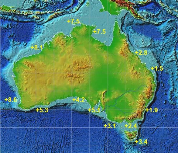
released a Queensland Ports Strategy that proposes to restrict any significant port development
adjoining the Great Barrier Reef World Heritage Area to within existing port limits until 2022. In
addition, the Australian and Queensland Governments prepared comprehensive Strategic
Assessments for the marine and coastal environments (GBRMPA 2013a, QDSDIP 2013) as well as
complementary Program Reports (GBRMPA 2013b) describing remedial actions to be taken in the
next decade. Both Program Reports commit to a future reef-wide integrated monitoring and
reporting program to underpin an adaptive management approach for this very large ecosystem. An
effective integrated monitoring framework must include a layer of ocean observations.

2.2 South East Queensland
South East Queensland (SEQ) is an area of outstanding natural values with its own legacy of
environmental issues; largely driven by very rapid expansion to accommodate the majority of the
State’s population in this region. The Gold Coast is Australia’s most highly concentrated tourist
destination and contributes more than $4B annually to the economy. Commercial fisheries in the
region are worth more than $50M annually, and the recreational fishing sector in the greater
Brisbane area generates many times more value.

Marine environments of the region include the Gold and Sunshine Coasts, Moreton Bay and Great
Sandy Marine Parks. The iconic sand islands (Fraser, Moreton, and Stradbroke) are precious natural
assets. Beach erosion is a significant threat to infrastructure because so much of the coast is sandy
and this is in most parts an open coast facing an energetic ocean. The outstanding biodiversity
values of SEQ include globally significant populations of sea turtles and dugongs, and annual
shorebird migrations that have led to Moreton Bay being listed as an international RAMSAR site.

South East Queensland has one of the fastest growing populations in Australia. The population,
which was 2.73 million in 2006, is predicted to exceed four million within 20 years. Such rapid
growth will make strong demands on natural resources such as Moreton Bay and the rivers and
streams feeding into it. The social costs of a decline in natural resource condition due to both local
and global (e.g. climate change) are very substantial. It is estimated that the social costs in SEQ alone
could be as high as $5.2 billion between now and 20311. Initiatives such as the SEQ Healthy
Waterways Partnership and the Gladstone Healthy Harbours Program have been established to help
mitigate and manage such risks. Such initiatives cannot succeed without systematic environmental
monitoring and reporting programs to measure the performance of management actions and for
essential communication of status and trend reporting to the stakeholder network.

2.3 Torres Strait and Gulf of Carpentaria
The Torres Strait is a narrow waterway between Australia and Papua New Guinea that separates the
Coral Sea in the east from the Arafura Sea in the west via the Gulf of Carpentaria. This shallow strait
contains almost 300 islands, of which 17 have permanent settlements supporting around 7,000
people. These islands have been occupied for several thousand years by indigenous peoples who
have a deep attachment to place and strong cultural and economic dependency upon local marine

1
 Binney J. 2010 Managing what matters: The cost of environmental decline in South East Queensland
Marsden Jacob Associates, 2010

                                                                                                        8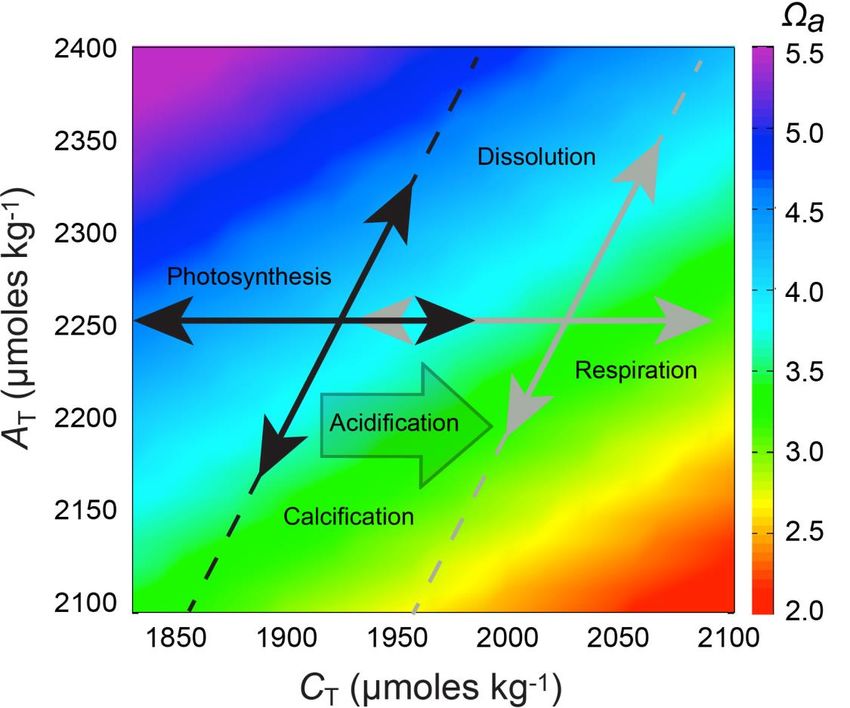
resources. In addition, there is an even larger diaspora of Torres Strait people living in the coastal
cities of north Queensland, who maintain active connections with their ancestral home lands.

While the environmental values of the Torres Strait compare favourably with more developed areas
of the Australian coastal, they will not remain so without active management of potential risks and
inevitably some adaptation. The Torres Strait now contains the largest population of dugongs in the
World and is the final global refuge for these charismatic herbivores as their populations have
declined elsewhere. In Queensland, the incidental catches of dugongs by the shark-netting program
record a 95% decline in abundance along the developed coast since the inception of the program
(Marsh et al. 2005) that is coincident with deep decline in their major food: seagrass. The Torres
Strait contains the largest contiguous seagrass meadow in tropical Australia, which would be at risk
from changes in water quality. These changes are less likely to be generated by local activities than
by future industrialisation, deforestation, and human development occurring in Papua New Guinea
and Irian Jaya. These risks of coastal pollution will interact with anthropogenic climate change.
Torres Strait populations on low-lying islands have critical vested interest in sea-level rise because
they already experience episodic tidal inundation of their lands and are at great risk from storm
surge.

The Gulf of Carpentaria (GOC) is a large shallow sea west of the Torres Strait that is bounded by land
on three sides and the Arafura Sea to the west. It covers 300,000 km2 with a maximum depth of 70m.
The region contains
600
    anomalies from 1901-81 mm          wet

                                400

                                200

                                  0

                                -200
                                       dry
                                -400
                                   1600 1640 1680 1720 1760 1800 1840 1880 1920 1960 2000
                                                            year

 Figure 2. Rainfall anomalies (relative to the average between 1901-1981) in North Queensland over
 300 years reconstructed from coral luminescence showing an extended natural drought 1760-1860
 followed by 100 years of alternation between wet and dry periods each lasting 2-10 years (source:
 Lough 2011).

The scale and complexity of this problem is very challenging and beyond simple empirical monitoring
because the largest flood plumes can extend many hundreds of kilometres along the coast, mixing
along the way with plumes from other catchments. Hence the risk profile at any location is the
historical accumulation of multiple impacts from water quality and other stresses.

A marine science partnership is meeting this challenge by creating an integrated modelling suite
known as eReefs (Schiller et al. 2013). This is designed to become a real-time forecasting system
operated by the Australian Bureau of Meteorology in an extension of its role as the nation’s weather
forecasting agency. Both systems share many similarities including the need for essential
observations.

In the marine space, eReefs is a 3-D hydrodynamic model that includes all of the essential forcing
functions (winds, tides, atmospheric coupling, bathymetry, etc). It is resolved at 1km grid resolution
on the continental shelf and nested within 4km and 10km models at progressively larger scales to
obtain accurate oceanic forcing from global models (Figure 3). The domain of the 4km grid extends
from Papua New Guinea to the NSW border (encompassing the east coast of Queensland) and
encompasses all of the shallow bathymetry on the Coral Sea (Queensland and Marion Plateaux).

                                                                                                     10
Figure 3. Spatial domain for eReefs model resolved at 4 km. Most of the domain where bathymetry is
less than 1000 m (yellow-red) is covered by a nested grid resolved at 1 km (Source Richard Brinkman,
AIMS).
11The eReefs model of ocean physics is validated using data from the QIMOS node, tide gauges
and Waverider buoys operated by the Queensland Government and Argo floats. . The QIMOS
array of delayed mode moorings provides spatial coverage from Lizard Island to the
Capricorn Bunker Group, and delivers time series of water column current profiles, and
temperature and salinity at a number of fixed depths on each mooring. The model has been
shown to capture key properties of the water column including temperature, salinity, and velocity
(Figure 4), and these capabilities allow the model to forecast thermal and salinity stress, track the
movements of flood plumes, and estimate shear at the seabed.
Figure 4. eReefs predicts temperature, salinity, and velocity at 47 depth layers resolved on either a 4km
or 1 km grid (Source Richard Brinkman, AIMS).
The hydrodynamic model will be coupled at the same resolution to models for sediment transport
and biogeochemistry (Figures 5,6).The coupled models under development will allow the integrated
suite to predict sediment transport on the seabed, wave resuspension, turbidity, water clarity,
benthic light levels and key attributes of the pelagic primary producers (standing stock, primary
production, size spectrum of phytoplankton).
eReefs is planned to be an essential part of an integrated monitoring framework for the GBR
(committed to in the GBR Strategic Assessments of the Australian and Queensland Governments)
but it will also have equal application to south east Queensland.
SEQ is Australia’s fastest growing region, with the population predicted to grow from 2.8 to 4.4
million people in the next 20 years. This rapid growth will need careful management to ensure that
local receiving waters are not degraded with impacts on seafood supply, livelihoods, and /or
12recreational opportunities. The SEQ Healthy Waterways Partnership has developed its own model of
water quality for the internal waters of Moreton Bay and the Gold Coast waterways. The open
boundary of this regional model will be forced by eReefs to transmit observed oceanic variability of
the EAC, which reaches its most forceful state at this latitude.
13Figure 5. The eReefs modelling suite when operational in 2015 will consist of coupled models producing predictions at the scale of the grid for biogeochemical
variables, sediment transport (dotted line). The ultimate goal is to predict ecological state (Source Richard Brinkman, AIMS).
14Figure 6. Traditional box model of phosphorus dynamics showing exchanges and transformations in
functional spatial compartments (Source Monbet et al. 2007). Ultimately eReefs will resolve these
processes to the nested grid sizes (4km, 1km, 0.1km).
In addition to forecasting water quality, eReefs will provide context for understanding and
forecasting the movement of migratory animals along the Queensland Shelf, variations in the
replenishment of major fisheries and the occurrence of toxic algal blooms and fish kills. It will also
assist maritime operations including search and rescue, contaminant spill response, and forecast risk
of tidal surge and beach erosion in coastal communities. The potential audience for this information
includes government, industry, and community. The uptake of the information and usefulness of the
forecasts will depend on their reliability and accuracy. As with conventional weather forecasting
models, this will be ensured to the fullest extent possible by data assimilation and forcing the
models with real-time observations.
This is how an ocean observing system in Queensland could deliver the greatest value to society.
Summary: Q-IMOS will make sustained observations so that oceanic variability can be included in
better evidence-based management decisions for a broad range of issues. For example, data on the
EAC will provide valuable information to meteorologists and planners because warm-core gyres can
affect the strength of destructive east coast lows, which in turn impact water supplies, coastal
erosion, and the integrity of infrastructure. In north Queensland, the equivalent knowledge is better
prediction of tropical cyclone tracks and intensities. In SEQ, more knowledge is required about how
the EAC influences coastal currents crucial to marine sediment transport. Coastal currents also
impact marine biodiversity with implications for ecotourism as well as Fisheries Management and
15Marine Park planning. Oceanographic processes affect the productivity of marine ecosystems as well
as the movements and migrations of animals in coastal waters.
Data collected by Q-IMOS will contribute to better outcomes for fisheries management and
conservation planning through incorporating knowledge about oceanic forcing into decision support
systems. The principal tool for predicting risk and impact will be the eReefs modelling suite, which
will be calibrated and validated by the sparse network of in situ observations collected by the IMOS
infrastructure.
163 Scientific Background, by Major Research Theme
The IMOS National Science and Implementation Plan is built on five ocean science themes and each
of them has at least partial relevance to Queensland. Hence the Q-IMOS Node Plan starts with
defining the areas of interest under the following topics:
Multi-decadal ocean change: monitoring broad-scale changes in the surface layers of the Coral
Sea as potential long-term drivers of coastal and marine ecosystems in Queensland
Modes of climate variability and extreme weather events impacting Queensland’s coastal and
marine ecosystems
Boundary currents and interbasin flows on Queensland’s continental margin
Continental shelf processes impacting Queensland’s coastal and marine ecosystems
Biological responses to ocean variability in Queensland’s coastal and marine ecosystems
3.1 Multi-decadal ocean change
3.1.1 The global energy balance (temperature) and sea level budget
Accurate and sustained observations of global surface temperatures began in the 19th century.
Subsequent monitoring has shown that the planet has warmed over the last 1600 years (Figure 7)
and continues to do so. This is consistent with the scientific consensus that anthropogenic impacts
have been responsible for a large portion of the global warming observed since the mid-20th century
(IPCC-ARS in press). On average, surface sea temperatures around Australia have increased by about
0.6-0.74°C over the past century (Lough and Hobday 2011; Lough et al. 2012). If the rate of warming
observed over the last 30 years were to continue throughout the 21st Century, average temperatures
on the GBR will be warmer by more than 1°C compared with the average for the last century (Figure
8). However, there is evidence that the rate of warming is accelerating and many climate models
predict warming of up to 3oC on our current global trajectory of increasing greenhouse gas emissions.
Figure 7. Global temperature anomalies relative to a 1961-1990 baseline
(source www.cru.uea.ac.uk)
17Figure 8. Sea temperatures from the GBR 1871-2005 with model forecasts (source
Janice Lough, AIMS)
Long-term changes in temperature associated with global warming are considered the greatest
threat to the survival of coral reefs in the next 100 years (Hoegh-Guldberg 1999, 2009). Efficient
reef-building is dependent on an intimate symbiosis between an animal host (the coral polyp) and
internal unicellular dinoflagellates (the symbionts) known as zooxanthellae. The symbionts capture
energy via photosynthesis and provide the animal host with nutrition. This energetic contribution
from the plant-like zooanthellae accounts for the ability of scleractinian corals to build coral reefs.
Natural selection has resulted in symbioses that operate most efficiently near the upper thermal
tolerance of the local combination of coral and zooxanthellae genotypes. As a result of this fine
balance, the coral-algal symbioses can be destabilised by several external stresses including thermal
stress (Berkelmans et al. 2004, 2010), excess light (Lesser and Farrell 2004), low salinity waters
(Kerswell and Jones 2003, Fabricius 2005, Berkelmans et al. 2012) and excess nutrients (Wooldridge
2009). When placed under stress, the animal host ejects its endosymbionts and the loss of their
pigments results in colonies of bleached appearance. If the corals remain in a bleached state for
more than a few days, the coral animal starves and dies.
Since the local thermal environment is a primary driver of coral bleaching and mortality, sea
temperature is one of the most important variables to be monitored in the Great Barrier Reef.
As the upper layers of the global oceans have warmed, thermal expansion has also forced a slow rise
in sea levels. Since 1870, the global average sea level has risen by ~250 mm. Sea levels rose at an
average of 1.7 mm.yr-1 during the 20th century but by about 3.1 mm.yr-1 from 1993 when sea level
began to be tracked by high accuracy satellite altimeters (Figure 9).
18Figure 9. Changes in Global Mean Sea Level between 1870 and 2009 (source
www.cmar.csiro.au/sealevel/).
Sea level rise has not been uniform, and in Australia, since 1993, sea levels have risen 7-10 mm to
the north and west of the continent but only 1.5-3 mm in Queensland (Figure 10). Nonetheless, sea
level rise has importance to low-lying communities, for example in the Torres Strait (Green et al.
2010), and for species that use the littoral zone for critical life stages (Fuentes et al. 2010. It is
recognition that the National Tidal Facility (Bureau of Meteorology) is monitoring coastal sea levels
at a number of established reference sites in Queensland, and Q-IMOS NSIP does not include any
commitment to monitor sea-level rise..
Net relative sea-level
trend mm/yr early 1990s
to June 2009
Figure 10. Sea level anomalies observed around the Australian coast
19
(source: www.bom.gov.au/ntc/IDO60202/IDO60202.2009.pdf).3.1.2 The global ocean circulation
Evidence is growing to suggest that the South Equatorial Current (SEC) flowing into the Coral Sea will
experience long-term change (Roemmich et al. 2007) reflecting a strengthened South Pacific Gyre
caused by stronger southeast trade winds. Climate modelling by Cai et al. (2005) has found that the
poleward EAC (see 2.3.1) will strengthen in the Tasman Sea due to the Southern Annular Mode
causing lighter mid-latitude winds and stronger southern ocean westerlies. Further climate scenario
modelling presented in Ganachaud et al. (2009) has shown an overall decrease in the SEC in
equatorial regions but an increase in its strength across a narrow band at 12°S and a broadening of
the SEC in the southern approaches to the Coral Sea (Figure 11). The cause of this in the models is a
decrease in equatorial winds, and an increase in strength and rotation to a more easterly component
of the SE trade winds in the subtropical Pacific. The increase in the southern branch of the SEC is at
the expense of the seasonal South Equatorial Counter Current (SECC) and will reinforce the flow of
the EAC into the Tasman Sea; an area that is already experiencing some of the fastest rates of ocean
warming in the world’s oceans (Ridgway 2007).
Figure 11. Projected changes to flow (in Sverdrups) for the major Pacific current systems. The
data are from the mean of 11 IPCC class coupled climate models under IPCC scenario A2
projected to 2090 relative to 1990 (averaged 1980-1999) transports (Source: Ganachaud, 2009).
Changes in the major circulation patterns of the atmosphere and the oceans raise questions about
the future strength and frequency of oceanic eddy production which is a major contributor to net
flow, and the extent of upwelling regions that will affect biological productivity. Ganachaud et al.
(2009) predict reduced productivity in tropical marine ecosystems due to shallowing of the surface
mixed layer caused by increased stratification (stronger warming, weaker winds) and a resulting
decrease in upwelling activity (3.4.2).
203.1.3 The global hydrological cycle (salinity)
Global climate models predict an amplification of the global hydrological cycle in the future, which
means dry areas getting drier and wet areas getting wetter (Durack et al., 2012; Biasutti 2013). There
is still inconsistency among multi-model climate projections for the Wet Tropics of the northern
coast of Queensland as to whether the summer monsoon will show an overall increase or decrease
in average rainfall. It is, however, clear that there is likely to be an increase in rainfall variability, i.e.
wet years will be wetter and dry years drier than present. A major driver of this rainfall and river
flow variability are El Niño-Southern Oscillation (ENSO) events, with El Niño years characterised by
drier than usual conditions and La Niña years by wetter than normal conditions (Risbey et al., 2009;
Ward et al. 2010). There is still, however, a lack of consistency between global climate models as to
how the frequency and/or intensity of ENSO events may change in a warmer world (Collins et al.,
2010; Guilyardi et al., 2012). We must assume, therefore, that ENSO events will be a continued
source of rainfall and river flow variability in the region but superimposed on warmer sea surface
temperatures (unusually warm SSTs around northern Australia contributed to the extensive flooding
associated with the 2010-2011 and 2011-2012 La Niña events2) and their considerable impacts both
on land and at sea (e.g. Holbrook et al., 2012). Northeast Australian rainfall and river flow variability
and linkages with ENSO activity are also modulated on inter-decadal timescales through the Pacific
Decadal Oscillation (PDO)/Interdecadal Pacific Oscillation (IPO) (Power et al. 1999). During PDO cool
phases, the teleconnections between ENSO and eastern Australian rainfall tend to be stronger with
more coherent rainfall anomalies and higher rainfall variability than during PDO warm phases (e.g.
Verdon et al., 2004). Again, it is unclear from the current generation of global climate models how
PDO may change in a warming world. As riverine export is the major driver of coastal water quality,
a regional marine observing system must have comprehensive data on rainfall and river discharges.
Suitable monitoring networks are in place and being maintained by the Bureau of Meteorology and
Queensland agencies (e.g. Environment and Heritage Protection).
3.1.4 The global carbon cycle (Inventory, air sea fluxes, physical controls)
Atmospheric carbon dioxide was just 280 ppm when James Watt patented his improved steam
engine in 1770. Since the Industrial Revolution in the 18th century, the burning of fossil fuels as a
cheap source of energy has injected massive quantities of carbon dioxide (CO2) to the global
atmosphere (Figure 12). Since CO2 is the main greenhouse gas, this increased atmospheric
concentration has trapped more heat in the atmosphere resulting in observed global warming.
Anthropogenic forcing is considered to be the major driver of global warming since the mid-20th
century (IPCC-AR5, in press).
About a third of the carbon dioxide released into the atmosphere from burning fossil fuels has been
absorbed into the global oceans (Raven et al. 2005). The rising partial pressure of CO2 dissolved in
seawater is making the oceans less basic and slightly more acidic (Doney et al. 2009). This trend
towards increasing pCO2 and reducing pH has been monitored at a number of ocean reference sites
including Station ALOHA: a deep ocean research site 100 km north of Oahu, Hawaii. Monthly
observations from that site have confirmed that surface pH has dropped by slightly less than 0.1
units since the industrial revolution (Figure 13a), and current estimates are that it could drop by a
further 0.3 to 0.5 units by 2100 as the oceans absorb more anthropogenic carbon.
2
http://www.bom.gov.au/climate/enso/history/La-Nina-2010-12.pdf
21Figure 12. Monthly sampling of CO2 levels in the atmosphere from sites in Hawaii
and north Queensland (source: World Data Centre for Greenhouse Gases
http://ds.data.jma.go.jp/gmd/wdcgg/).
These small changes in ocean chemistry could have a profound consequence for all marine
organisms building calcareous body structures (shells, skeletons, fish otoliths). Such structures are
vulnerable to dissolution unless the surrounding seawater contains saturating concentrations of
carbonate ions. Recent changes are reducing the saturation states of aragonite and calcite (Figure
13b,c), the two most important crystal forms of CaCO3. Impacts of these changes are still poorly
known (Hendriks et al. 2010), but theoretically they are great enough to pose a significant challenge
to all marine biological calcification because ocean pH is falling at rates not experienced for many
millions of years and associated with episodes of mass extinction of marine life (Hoegh-Guldberg et
al. 2007, Veron et al. 2009).
22Figure 13. Time series of atmospheric CO2 and responding ocean variables from a deep ocean
reference site off Hawaii based on monthly sampling (source Doney et al. 2009). GEOSECS data
were collected in 1973 from a station near ALOHA.
233.1.5 Science Questions
As a coastal observing Node, Q-IMOS does not collect many observations off the continental shelf
and obtains the necessary reference data from the Bluewater and Climate Node. Q-IMOS will be a
user of data on multi-decadal change rather than a generator of mechanistic hypotheses or source
of predictions. The Q-IMOS data streams will capture regional dynamics and therefore provide
observations useful for calibrating some of the models of these larger processes.
The Queensland Node observing strategy will contribute to the following high-level science
questions from the National Plan:
Ocean Heat Content:
Are changes in ocean temperatures in the Coral Sea similar at all depths?
Do changes in ocean temperatures in the Coral Sea change the depth of the mixed layer?
Do Coral Sea temperature variations drive changes in temperature on the continental shelf?
Global carbon budget:
Do changes in pCO2/pH on the GBR shelf mirror trends observed at deep ocean reference sites?
Q-IMOS seeks to know whether changes in the heat content of the Coral Sea drive changes in
temperature on the continental shelf and requires information on the pCO2/pH of oceanic water as
a reference state for changes observed in shelf waters and ecosystems. It will also collect data on
shelf salinity that be linked with multi-decadal changes in rainfall and river discharge.
3.1.6 Notable gaps and future priorities
Notable gaps:
While there are a number of ARGO floats that sample oxygen, there is the need for increased data
density in the Coral Sea and along the margins of the QLD shelf.
Future priorities:
Sea Gliders to observe bio-physical properties of the upper global ocean adjacent to the QLD shelf
Slocum Gliders for repeat cross-shelf transects bio-physical properties.
3.2 Climate variability and weather extremes
3.2.1 Interannual Climate Variability
3.2.1.1 El Niño –Southern Oscillation (ENSO)
Interannual climate variability over the Pacific is dominated by the El Niño–Southern Oscillation
(ENSO) cycle, which is a quasi-periodic climate pattern of ocean and atmospheric anomalies across
the tropical Pacific Ocean (McPhaden et al. 2006). In the atmosphere, this corresponds with the
east-west migration of the Walker overturning circulation (Figure 14), which can be tracked (and
predicted) by the difference in atmospheric pressure across the Pacific Ocean. The Southern
Oscillation Index (SOI) is a measure of the difference between air pressure in Darwin and Tahiti,
although multivariate proxies involving more stations are becoming the norm in models seeking
24better prediction of response variables like rainfall. The SOI varies between extreme states at
intervals of three to seven years.
Figure 14: ENSO cycle showing La Niña (left), neutral (centre), and El Niño (right) states (source
www.pmel.noaa.gov/tao/elnino/nino-home.html).
Warm tropical waters are a major evaporative source of rain-bearing clouds. Although the ocean-
atmosphere forcing is still a subject of study, it is clear that the east-west position of the warm pool
in the ocean along the equator is correlated with similar change in the longitude of the atmospheric
changes; hence the name ENSO. The extreme states of this coupled atmosphere-ocean system are
when the warm pool in the ocean and the major uplifting convection cell in the atmosphere are in
the western Pacific (known as the La Niña phase) and the opposite condition when both have moved
to their extreme position in the central Pacific (known as El Niño phase).
El Niño episodes have long been recognised in the eastern Pacific (Wyrtki 1984) as the arrival of
warmer surface waters that depress the thermocline shutting off the coastal upwelling that normally
supports productive scale fisheries in the Americas. In the neutral state, trade winds drive hot
equatorial surface water to the western Pacific, where it forms the West Pacific Warm Pool (WPWP)
and upwelling occurs in the eastern Pacific to replace these surface waters (McPhaden et al. 2006)
La Niña episodes represent the extreme opposite state when strong surface winds have pushed the
WPWP to its western limit (noting that topography sets a limit on this displacement). In this
alternate state, the thermocline in the western Pacific is depressed at the same time as it rises to the
surface in the eastern Pacific to compensate for the volume of surface water being driven westwards.
These quasi-cyclic reverberations have strong and opposite influences on a range of variables
(temperature, rainfall, wind, storminess, and upwelling) on both sides of the oceanic basin so that
ENSO is a major source of climate variation impacting on ecosystems and sovereign economies.
Figure 15 shows an example of the impact of ENSO upon coastal currents with practical implications
for port operations (e.g. dredge spoil disposal).
25Figure 15. Surface large-scale currents for El Niño (2004), and La Niña
(2011) phases at three major ports in north Queensland (source: GBRMPA
2013a).
In the 20th century, the strongest ENSO events were 1982/83 (Tang and Weisberg 1984) and 1997/98.
Since the underlying phenomenon is the strength of the equatorial currents across the Pacific (SEC in
the Southern Hemisphere), the SOI signal in the atmosphere is mirrored by sea levels in the Western
Pacific (Figure 16) albeit with an attenuated signal on the north Queensland coastline.
26Figure 16. (Top) SOI index, (Middle) Sea levels from tide gauges in PNG, Solomon Islands (Lower)
Sea levels from NE Australia (sources below).
http://reg.bom.gov.au/climate/current/soi-1993-2000.shtml
http://www.bom.gov.au/oceanography/projects/abslmp/abslmp.shtml
http://www.bom.gov.au/oceanography/projects/spslcmp/spslcmp.shtml
Ridgway et al. (1993) examined an ENSO event from 1986-87 that was of similar magnitude and the
same sign as the 1997-98 event shown above. Although not as severe as the very strong El Niño of
1982/83, mean sea level at Honiara (Solomon Islands) dropped by 25 cm in early 1987. Their
modelling of data from tide gauges and XBT casts showed a large region of depressed sea level
centred on Honiara within a zonal band between the equator and 15°S (Figure 17).
This depression was steeply contoured between 150-165°E especially in the Solomon Sea, implying
strong westward geostrophic flow in the south and the opposite in the north. The crowding of the
27contour lines in the Solomon Sea shows very strong NW flow along the PNG coastline and the
authors estimated a flow anomaly of 15 Sv through the Vitiaz Strait, and a similar enhancement of
flow through the nearby Solomon Straits. They also commented on the lack of response along the
Australian coast between 10-30°S and from the tide gauge at Port Moresby interior to the Gulf of
Papua. This suggests that much of the extra flow in the northern part of the SEC during El Niño
episodes is channelled directly into the Solomon Sea.
Figure 17. Contours of sea level anomalies (source Ridgway et al. 1993).
Notwithstanding this observation, the southern arm of the SEC and hence the EAC (see next section)
should also strengthen during El Niño episodes due to the southern displacement of the SEC by
WPWP water flowing east along the equator (Wrytki 1984, Meyers and Donguy 1984, Johnston and
Merrifield 2000). Burrage et al. (1994) observed a strengthening of the EAC adjacent to the central
GBR but Ridgway (2007) found only a very weak ENSO signal with a nine month lag in observations
from the Maria Island site in Tasmania. He also suggested that this signal was delivered to south-east
Australia from the Indonesian Through-flow in north Western Australia after propagation along the
coastal wave guide. The most distant expression of this connectivity is the coupled dynamics of the
poleward Zeehan Current flowing down the west coast of Tasmania.
In 3.1, the multi-decadal trend in ocean temperatures is described. A major anomaly in that trend
occurred between 1945 and 1977 (Figure 7). The overall temperature increase of the Southern
Hemisphere for the period 1946–1975 was only 0.06°C compared with 0.14°C for the period 1976–
1998 (Salinger et al. 2001). These multi-decadal cycles have been correlated with a basin-scale
pattern of sea surface temperature and pressure anomalies expressed away from the equator in
both hemispheres known as the Inter-decadal Pacific Oscillation (IPO) or Pacific Decadal Oscillation
(Mantua et al. 1997).
28The IPO/PDO (Figure 18) is a low frequency signal in sea surface height and sea surface temperatures
reflecting slow internal processes in ocean mixing and circulation in the Pacific Ocean that can
obscure global trends in the climate. This oscillation specifically separates alternating periods, each
lasting 2-3 decades, of different warming patterns with effects on temperature, rainfall, and winds.
Figure 18. Index showing phases of the IPO (source
www.bom.gov.au/climate/cli2000/jimSal.html)
The IPO signal as defined from Meteorological Office HadISST data shows positive phases in 1922–
1944 and 1978–1998, and a negative phase between 1946 and 1977 (Salinger et al. 2001). These
periods correspond with sustained heating and cooling episodes in global temperatures (Figure 7).
When the IPO is in a positive phase, SST anomalies over the North Pacific and near New Zealand are
negative, whereas SST anomalies over the tropical Pacific are positive. In the negative phase, these
patterns are reversed.
The pattern and timescale of IPO variability has been attributed to atmospheric teleconnections
from the Tropics (i.e. ENSO variability) to the extra tropics (known as the Pacific-South American
Mode), followed by extra tropical oceanic teleconnections propagating westwards in the form of
baroclinic Rossby waves. As the latter take over a decade to cross an ocean at subtropical latitudes,
they are thought to dictate the temporal scale of basin-scale decadal variability and hence the
broader spatial pattern of decadal ENSO (Power et al. 2006; Sasaki et al. 2008). Since Rossby waves
act as ‘integrators’ of wind forcing as they propagate across the Pacific, the response of the
extratropical ocean has been thought of as a low pass filter of high frequency atmospheric variability
(Sasaki et al. 2008).
Power et al. (1999) showed that the two phases of the IPO strongly modulate the relationship
between ENSO and rainfall variability over Australia. Specifically there is no clear relationship
between interannual variations in the Australian climate and ENSO during warm phases of the IPO
but robust relationships during cold phases of the IPO between ENSO and variability in rainfall and
surface temperature. The strong ENSO event in 1997/98 is thought to have been reinforced by an in-
phase IPO (Burgman et al., 2008).
293.2.2 Intra-seasonal variability and severe weather
Most of the physical phenomena to be captured by an Integrated Marine Observing System have
annual cycles, which in many cases are driven ultimately by the seasonal patterns of global surface
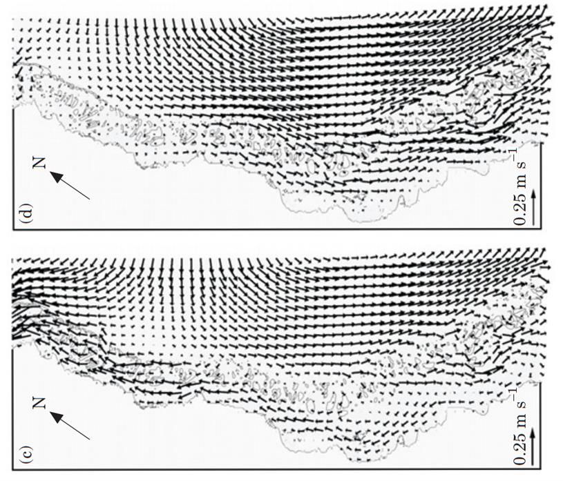
heating due to the earth’s orbit. For example, the bifurcation of the westerly flows in the Coral Sea
(Figure 19) at the surface moves south during the season of SE trade winds (April-November). During
the summer monsoon, southerly flows contributing to the EAC start near 15°S. In the winter, the
coastal bifurcation is found nearer to 18°S. Figure 19 suggests that this is due to a different fate for
surface flow steered to the north of the Queensland Plateau. Given the implied influence of the wind
fields, this displacement is likely to vary among years.
Figure 19. Coral Sea circulation inferred for the upper 1000m in October 1985; SEC – South
Figure
Equatorial27. Coral
Current; EACSea
– Eastcirculation inferred
Australian Current; for
HC – Hiri the (source
Current upperBurrage
1000m in
1993)
October 1985; SEC – South Equatorial Current; EAC – East
Ridgway and Godfrey (1997) detected a strong seasonal cycle in the open ocean zonal geostrophic
Australian Current; HC - Hiri Current (source Burrage 1993).
transport north of 25°S and a similar strong seasonal cycle in the EAC down the Australian coastline
between 25-45°S, with the strongest southward flow observed during the austral summer. They also
showed that the amplitude of this seasonal cycle in the EAC strength diminished with southward
progression especially below Sydney (34°S).
While average sea temperature across the GBR has increased by about 0.4°C since the 19th century
(Figure 8, Lough 2007), interannual variations within a decade at fixed sites have larger amplitude
and is a key factor affecting the risk of coral bleaching. Figure 20 shows three historical bleaching
episodes on the GBR coincident with summer maximum water temperatures about 1°C above the
flanking years. All three events occurred during years with strongly negative SO indices indicative of
El Niño episodes. However the index was equally strong with the same sign in 1993 and 1997 (Figure
20), which remained cooler and without bleaching. The 1996/7 summer experienced five tropical
cyclones between January and March, which collectively drew a lot of heat from the Coral Sea and
may have reduced heat stress along the GBR.
30Magnetic Island - Reef-slope
Average daily temperature
34 Bleaching Bleaching Bleaching
32
30
28
(°C)
26
24
22
20
18
Jan-91
Jan-92
Jan-93
Jan-94
Jan-95
Jan-96
Jan-97
Jan-98
Jan-99
Jan-00
Jul-90
Jul-91
Jul-92
Jul-93
Jul-94
Jul-95
Jul-96
Jul-97
Jul-98
Jul-99
Jul-00
Figure 20. Interannual variations in temperature on the reef slope at Magnetic Island (source
Madeleine van Oppen, AIMS).
Schiller et al. (2009) reanalysed the conditions prevailing during three episodes when the Coral Sea
showed significant SST anomalies (including that caused by TC Justin in 1997). They found that the
dynamics of all three events were different due to a unique mix of local and remote influences,
which points to the difficulty of interpreting interannual variation without observational data.
3.2.2.1 The Madden-Julian Oscillation (MJO)
The northern Australian summer monsoon is also modulated on 30-50 day timescales by the MJO
(Risbey et al. 2009). This is a large-scale eastward moving atmospheric wave-like disturbance along
the equator mainly operating between the Indian and Pacific Oceans. As it passes through a given
region, it can enhance or suppress convective activity and thus can lead to bursts and breaks in the
northern Australian summer monsoon (Wheeler et al., 2009).
The MJO is classified into eight phases based on the pattern of convection and zonal winds in near
equatorial latitudes and its phase is tracked in near-real time by the Bureau of Meteorology
(http://www.bom.gov.au/climate/mjo/). Passage of the MJO, by enhancing/suppressing monsoonal
activity not only affects rainfall but also can lead to surface water cooling or warming at critical times
for thermal stress events; thus influencing the risk of coral bleaching.
The MJO interacts with ENSO. In northern Australia, MJO-forced dry spells are drier in El-Niño years
than in La Niña years (Risbey et al. 2009). During winter, the rainfall response along the Queensland
coast co-varies with the MJO phase due to modulation of the SE trade winds. While the spatial
domain influenced by the MJO is not as great as for ENSO or IPO, the time domain is much shorter
with variation in wind and rainfall expressed at scales of days to weeks rather than seasons and
years.
313.2.2.2 Tropical Cyclones
Differences in the strength of the summer monsoon circulation over northern Australia associated
with ENSO events also result in marked differences in the occurrence of tropical cyclones along the
GBR, with reduced activity during El Niño years when the tropical warm pool has receded into the
east and enhanced activity during La Niña years (Lough 1994). Although there are several
environmental conditions required for tropical cylone formation, these highly energetic atmospheric
disturbances require SST above 26°C (Emanuel 2003). The recent record suggests slightly enhanced
activity during La Niña episodes in the western Pacific but the record of their tracks over the same
period shows that they have varied origins and diverse trajectories (Figure 21), which are only
predictable from knowledge of ocean temperatures and atmospheric conditions applying near and
following their formation.
Figure 21. (Left) Interannual variation in the number of tropical cyclones affecting northern Australia
(source: http://www.bom.gov.au/cyclone/climatology/trends.shtml). (Right) Cyclone tracks in the
Western Pacific (http://www.bom.gov.au/cyclone/about/eastern.shtml#history).
Due to their sporadic occurrence and tracks, there is, as yet, no clear evidence as to whether the
frequency and/or intensity of tropical cyclones in the southwestern Pacific has changed (Australian
Bureau of Meteorology and CSIRO 2011). Some come from the far field (distant western or eastern
origins) but severe tropical cyclones (Categories 4,5) impacting the Queensland coast inevitably
require a period of intensification over the adjacent Coral Sea.
Even though the long-term trend is unclear, the GBR has been impacted substantially by severe
(Category 4,5) tropical cyclones since 2005 (Figure 22). The cumulative exposure to cyclones since
1985 has been responsible for approximately half of an observed decline in coral cover (De’ath et al.
2012) across the whole GBR but the impacts have been much more severe in the southern GBR
(Figure 23).
The potential for these severe atmospheric disturbances to create extreme and anomalous weather
conditions is revealed by comparing the extent of fresh water flooding of the GBR observed in 2010-
11 with the average result from two decades of observation (Figure 22). In 2010-11, separate events
(TC Yasi and TC Oswald) resulted in exceptional rainfall in the Burdekin and Fitzroy catchments,
32You can also read