Risk Averse Robust Adversarial Reinforcement Learning
←
→
Page content transcription
If your browser does not render page correctly, please read the page content below
Risk Averse Robust Adversarial Reinforcement Learning
                                                                                    Xinlei Pan1 , Daniel Seita1 , Yang Gao1 , John Canny1

                                             Abstract— Deep reinforcement learning has recently made                                                           Competition

                                         significant progress in solving computer games and robotic con-
                                         trol tasks. A known problem, though, is that policies overfit to
                                         the training environment and may not avoid rare, catastrophic
                                                                                                                                     Maximize                                               Minimize
                                         events such as automotive accidents. A classical technique for                              Reward                                                 Reward
                                         improving the robustness of reinforcement learning algorithms
arXiv:1904.00511v1 [cs.LG] 31 Mar 2019

                                         is to train on a set of randomized environments, but this
                                         approach only guards against common situations. Recently, ro-                                          Protagonist:                  Adversary:
                                         bust adversarial reinforcement learning (RARL) was developed,                                          Risk Averse                  Risk Seeking
                                         which allows efficient applications of random and systematic
                                         perturbations by a trained adversary. A limitation of RARL                          Fig. 1: Risk averse robust adversarial reinforcement learning diagram: an
                                         is that only the expected control objective is optimized; there                     autonomous driving example. Our framework includes two competing agents
                                         is no explicit modeling or optimization of risk. Thus the                           acting against each other, trying to drive a car (protagonist), or trying to
                                         agents do not consider the probability of catastrophic events                       slow or crash the car (adversary). We include a notion of risk modeling
                                                                                                                             in policy learning. The risk-averse protagonist and risk-seeking adversarial
                                         (i.e., those inducing abnormally large negative reward), except                     agents learn policies to maximize or minimize reward, respectively. The use
                                         through their effect on the expected objective. In this paper we                    of the adversary helps the protagonist to effectively explore risky states.
                                         introduce risk-averse robust adversarial reinforcement learning
                                         (RARARL), using a risk-averse protagonist and a risk-seeking
                                         adversary. We test our approach on a self-driving vehicle                           We envision this as enabling training of more robust agents
                                         controller. We use an ensemble of policy networks to model                          in simulation and then using sim-to-real techniques [10] to
                                         risk as the variance of value functions. We show through                            generalize to real world applications, such as house-hold
                                         experiments that a risk-averse agent is better equipped to
                                         handle a risk-seeking adversary, and experiences substantially
                                                                                                                             robots or autonomous driving, with high reliability and safety
                                         fewer crashes compared to agents trained without an adversary.                      requirements. A recent algorithm combining robustness in
                                         Supplementary materials are available at https://sites.                             reinforcement learning and the adversarial framework is
                                         google.com/view/rararl.                                                             robust adversarial reinforcement learning (RARL) [11], which
                                                                                                                             trained a robust protagonist agent by having an adversary
                                                                     I. I NTRODUCTION
                                                                                                                             providing random and systematic attacks on input states and
                                            Reinforcement learning has demonstrated remarkable per-                          dynamics. The adversary is itself trained using reinforcement
                                         formance on a variety of sequential decision making tasks                           learning, and tries to minimize the long term expected reward
                                         such as Go [1], Atari games [2], autonomous driving [3],                            while the protagonist tries to maximize it. As the adversary
                                         [4], and continuous robotic control [5], [6]. Reinforcement                         gets stronger, the protagonist experiences harder challenges.
                                         learning (RL) methods fall under two broad categories: model-                          RARL, along with similar methods [12], is able to achieve
                                         free and model-based. In model-free RL, the environment’s                           some robustness, but the level of variation seen during
                                         physics are not modeled, and such methods require substantial                       training may not be diverse enough to resemble the variety
                                         environment interaction and can have prohibitive sample                             encountered in the real-world. Specifically, the adversary
                                         complexity [7]. In contrast, model-based methods allow                              does not actively seek catastrophic outcomes as does the
                                         for systematic analysis of environment physics, and in                              agent constructed in this paper. Without such experiences,
                                         principle should lead to better sample complexity and more                          the protagonist agent will not learn to guard against them.
                                         robust policies. These methods, however, have to date been                          Consider autonomous driving: a car controlled by the protag-
                                         challenging to integrate with deep neural networks and to                           onist may suddenly be hit by another car. We call this and
                                         generalize across multiple environment dimensions [8], [9],                         other similar events catastrophic since they present extremely
                                         or in truly novel scenarios, which are expected in unrestricted                     negative rewards to the protagonist, and should not occur
                                         real-world applications such as driving.                                            under a reasonable policy. Such catastrophic events are highly
                                            In this work, we focus on model-free methods, but                                unlikely to be encountered if an adversary only randomly
                                         include explicit modeling of risk. We additionally focus on                         perturbs the environment parameters or dynamics, or if the
                                         a framework that includes an adversary in addition to the                           adversary only tries to minimize total reward.
                                         main (i.e., protagonist) agent. By modeling risk, we can train                         In this paper, we propose risk averse robust adversarial
                                         stronger adversaries and through competition, more robust                           reinforcement learning (RARARL) for training risk averse
                                         policies for the protagonist (see Figure 1 for an overview).                        policies that are simultaneously robust to dynamics changes.
                                           1
                                                                                                                             Inspired by [13], we model risk as the variance of value
                                               University of California, Berkeley. {xinleipan,seita,yg,canny}@berkeley.edu
                                                                                                                             functions. To emphasize that the protagonist be averse to
                                                                                                                             catastrophes, we design an asymmetric reward function (see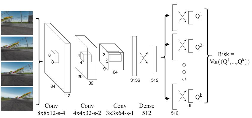
Section IV-A): successful behavior receives a small positive       sampling trajectories which may never encounter adverse
reward, whereas catastrophes receive a very negative reward.       outcomes, whereas with sparse risks (as is the case here)
   A robust policy should not only maximize long term              adversarial sampling provides more accurate estimates of the
expected reward, but should also select actions with low           probability of a catastrophe.
variance of that expected reward. Maximizing the expectation          A popular ingredient is to enforce constraints on an
of the value function only maximizes the point estimate of         agent during exploration [24] and policy updates [25], [26].
that function without giving a guarantee on the variance.          Alternative techniques include random noise injection during
While [13] proposed a method to estimate that variance, it         various stages of training [27], [28], injecting noise to the
assumes that the number of states is limited, while we don’t       transition dynamics during training [29], learning when to
assume limited number of states and that assumption makes          reset [30] and even physically crashing as needed [31].
it impractical to apply it to real world settings where the        However, Rajeswaran et al. [29] requires training on a target
number of possible states could be infinitely large. Here, we      domain and experienced performance degradation when the
use an ensemble of Q-value networks to estimate variance. A        target domain has a different model parameter distribution
similar technique was proposed in Bootstrapped DQNs [14]           from the source. We also note that in control theory, [32], [33]
to assist exploration, though in our case, the primary purpose     have provided theoretical analysis for robust control, though
of the ensemble is to estimate variance.                           their focus lies in model based RL instead of model free RL.
   We consider a two-agent reinforcement learning scenario         These prior techniques are orthogonal to our contribution,
(formalized in Section III). Unlike in [11], where the agents      which relies on model ensembles to estimate variance.
performed actions simultaneously, here they take turns                Uncertainty-Driven Exploration. Prior work on explo-
executing actions, so that one agent may take multiple steps       ration includes [34], which measures novelty of states using
to bring the environment in a more challenging state for the       state prediction error, and [35], which uses pseudo counts
other. We seek to enable the adversarial agent to actively         to explore novel states. In our work, we seek to measure
explore the parameter variation space, so that the perturbations   the risk of a state by the variance of value functions. The
are generated more efficiently. We use a discrete control          adversarial agent explores states with high variance so that it
task, autonomous driving with the TORCS [15] simulator, to         can create appropriate challenges for the protagonist.
demonstrate the benefits of RARARL.                                   Simulation to Real Transfer. Running reinforcement
                                                                   learning on physical hardware can be dangerous due to
                    II. R ELATED W ORK                             exploration and slow due to high sample complexity. One
   Reinforcement Learning with Adversaries. A recent               approach to deploying RL-trained agents safely in the real
technique in reinforcement learning involves introducing           world is to experience enough environment variation during
adversaries and other agents that can adjust the environment       training in simulation so that the real-world environment looks
difficulty for a main agent. This has been used for robust         just like another variation. These simulation-to-real techniques
grasping [16], simulated fighting [17], and RARL [11], the         have grown popular, including domain randomization [10],
most relevant prior work to ours. RARL trains an adversary         [36] and dynamics randomization [37]. However, their focus
to appropriately perturb the environment for a main agent.         is on transferring policies to the real world rather than training
The perturbations, though, were limited to a few parameters        robust and risk averse policies.
such as mass or friction, and the trained protagonist may be
vulnerable to other variations.                                          III. R ISK AVERSE ROBUST A DVERSARIAL RL
   The works of [12] and [18] proposed to add noise to state         In this section, we formalize our risk averse robust
observations to provide adversarial perturbations, with the        adversarial reinforcement learning (RARARL) framework.
noise generated using fast gradient sign method [19]. However,
                                                                   A. Two Player Reinforcement Learning
they did not consider training an adversary or training risk
averse policies. The work of [20] proposed to introduce              We consider the environment as a Markov Decision Process
Bayesian optimization to actively select environment variables     (MDP) M = {S , A , R, P, γ}, where S defines the state
that may induce catastrophes, so that models trained can be        space, A defines the action space, R(s, a) is the reward
robust to these environment dynamics. However, they did not        function, P(s0 |s, a) is the state transition model, and γ is the
systematically explore dynamics variations and therefore the       reward discount rate. There are two agents: the protagonist
model may be vulnerable to changing dynamics even if it is         P and the adversary A.
robust to a handful of rare events.                                  Definition. Protagonist Agent. A protagonist P learns a
   Robustness and Safety in RL. More generally, robustness         policy πP to maximize discounted expected reward EπP [∑ γ t rt ].
and safety have long been explored in reinforcement learn-         The protagonist should be risk averse, so we define the value
ing [21], [22], [23]. Chow et al. [23] proposed to model risk      of action a at state s to be
via constraint or chance constraint on the conditional value                  Q̂P (s, a) = QP (s, a) − λPVark [QkP (s, a)],      (1)
at risk (CVaR). This paper provided strong convergence guar-
antees but made strong assumptions: value and constrained          where Q̂P (s, a) is the modified Q function, QP (s, a) is the
value functions are assumed to be known exactly and to             original Q function, and Vark [QkP (s, a)] is the variance of the
be differentiable and smooth. Risk is estimated by simply          Q function across k different models, and λP is a constant;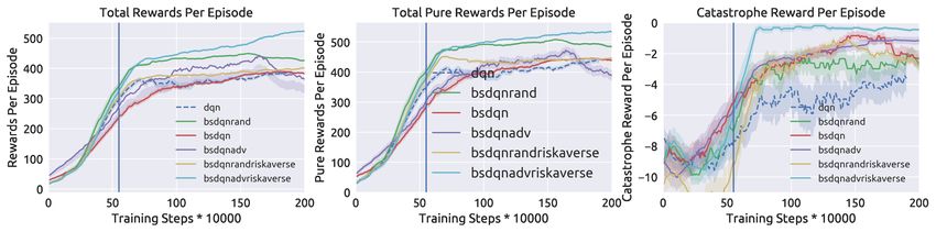
the variance of Q value functions by training multiple Q
                                                                               value networks in parallel. Hereafter, we use Q to denote
                                                                               the entire Q value network, and use Qi to denote the i-
                                                                               th head of the multi-heads Q value network.1 As shown
                                                                               in Figure 2, the network takes in input s, which consists
                                                                               of stacked frames of consecutive observations. It passes s
                                                                               through three shared convolutional layers, followed by one
                                                                               (shared) dense layer. After this, the input is passed to k
                                                                               different heads which perform one dense layer to obtain
                                                                               k action-value outputs: {Q1 (s, · ), . . . , Qk (s, · )}. Defining the
Fig. 2: Our neural network design. (Notation: “s” indicates stride for         mean as Q̃(s, a) = 1k ∑ki=1 Qi (s, a), the variance of a single
the convolutional weight kernel, and two crossing arrows indicate dense
layers.) The input is a sequence of four stacked observations to form an       action a is,
(84 × 84 × 12)-dimensional input. It is passed through three convolutional
                                                                                                              1 k
layers to obtain a 3136-dimensional vector, which is then processed through
a dense layer. (All activations are ReLus.) The resulting 512-dimensional
                                                                                          Vark (Q(s, a)) =      ∑ (Qi (s, a) − Q̃(s, a))2 ,
                                                                                                              k i=1
                                                                                                                                                    (3)
vector is copied and passed to k branches, which each process it through
dense layers to obtain a state value vector Qi (s, ·). We apply the ensemble   where we use the k subscripts to indicate variance over k
DQN framework for estimating the value function variance.                      models, as in Equations 1 and 2. The variance in Equation 3
                                                                               measures risk, and our goal is for the protagonist and
The term −λPVark [QkP (s, a)] is called the risk-averse term                   adversarial agents to select actions with low and high variance,
thereafter, and encourages the protagonist to seek lower                       respectively.
variance actions. The reward for P is the environment reward                      At training time, when we sample one action using the Q
rt at time t.                                                                  values, we randomly choose one of k heads from Q1 to Qk ,
   Definition. Adversarial Agent. An adversary A learns                        and use this head throughout one episode to choose the action
a policy πA to minimize long term expected reward, or                          that will be applied by the agent. When updating Q functions,
to maximize the negative discounted reward EπA [∑ −γ t rt ].                   our algorithm (like DQN [2]) samples a batch of data of size B
To encourage the adversary to systematically seek adverse                      from the replay buffer {(s, a, s0 , r, done)t }t=1
                                                                                                                              B   which, for each
outcomes, its modified value function for action selection is                  data point, includes the state, action, next state, reward, and
             Q̂A (s, a) = QA (s, a) + λAVark [QkA (s, a)],              (2)    task completion signal. Then we sample a k-sized mask. Each
                                                                               mask value is sampled using a Poisson distribution (modeling
where Q̂A (s, a) is the modified Q function, QA (s, a) is the                  a true Bootstrap sample with replacement) instead of the
original Q function, Vark [QkA (s, a)] is the variance of the Q                Bernoulli distribution in [14] (sample without replacement).
function across k different models, and λA is a constant;                      At test time, the mean value Q̃(s, a) is used for selecting
the interaction between agents becomes a zero-sum game                         actions.
by setting λA = λP . The term λAVark [QkA (s, a)] is called the
                                                                               C. Risk Averse RARL
risk-seeking term thereafter. The reward of A is the negative
of the environment reward −rt , and its action space is the                       In our two-player framework, the agents take actions
same as for the protagonist.                                                   sequentially, not simultaneously: the protagonist takes m
   The necessity of having two agents working separately                       steps, the adversary takes n steps, and the cycle repeats. The
instead of jointly is to provide the adversary more power                      experience of each agent is only visible to itself, which means
to create challenges for the protagonist. For example, in                      each agent changes the environment transition dynamics
autonomous driving, a single risky action may not put                          for another agent. The Q learning Bellman equation is
the vehicle in a dangerous condition. In order to create a                     modified to be compatible with this case. Let the current
catastrophic event (e.g., a traffic accident) the adversary needs              and target value functions be QP and Q∗P for the protagonist,
to be stronger. In our experiments (a vehicle controller with                  and (respectively) QA and Q∗A for the adversary. Given the
discrete control), the protagonist and adversary alternate full                current state and action pair (st , at ), we denote actions
control of a vehicle, though our methods also apply to settings                executed by the protagonist as atP and actions taken by the
in [11], where the action applied to the environment is a sum                  adversary as atA . The target value functions are QP (stP , atP ) =
                                                                                                             A , aA ) + γ n+1 max Q∗ (sP
                                                                               r(stP , atP ) + ∑ni=1 γ i r(st+i
of contributions from the protagonist and the adversary.                                                          t+i               a       t+n+1 , a),
                                                                               and, similarly,QA (st , atA ) = r(stA , atA ) + ∑m
                                                                                                       A
                                                                                                                                i=1 γ i r(sP , aP ) +
                                                                                                                                           t+i t+i
B. Reward Design and Risk Modeling                                             γ m+1 maxa Q∗ (st+m+1
                                                                                                  A       , a). To increase training stability for
  To train risk averse agents, we propose an asymmetric                        the protagonist, we designed a training schedule Ξ of the
reward function design such that good behavior receives small                  adversarial agent. For the first ξ steps, only the protagonist
positive rewards and risky behavior receives very negative                     agent takes actions. After that, for every m steps taken by
rewards. See Section IV-A and Equation 4 for details.                          the protagonist, the adversary takes n steps. The reason
  The risk of an action can be modeled by estimating the                         1 We use Q and Qi to represent functions that could apply to either the
variance of the value function across different models trained                 protagonist or adversary. If it is necessary to distinguish among the two
on different sets of data. Inspired by [14], we estimate                       agents, we add the appropriate subscript of P or A.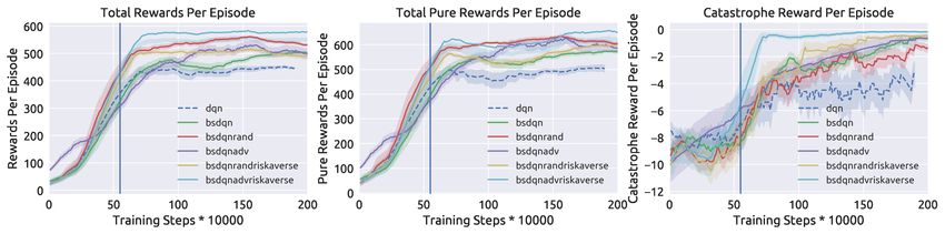
for this training schedule design is that we observed if the       do nothing, (6) move right, (7) move right and decelerate, (8)
adversarial agent is added too early (e.g., right at the start),   move ahead and decelerate, (9) move right and decelerate.
the protagonist is unable to attain any rewards. Thus, we let         We next define our asymmetric reward function. Let v
the protagonist undergo a sufficient amount of training steps      be the magnitude of the speed, α be the angle between the
                                                                   speed and road direction, p be the distance of the vehicle
to learn basic skills. The use of masks in updating Q value        to the center of the road, and w be the road width. We
functions is similar to [14], where the mask is a integer          additionally define two binary flags: 1st and 1da , with 1st = 1
vector of size equal to batch size times number of ensemble        if the vehicle is stuck (and 0 otherwise) and 1da =l 1 if the   m
Q networks, and is used to determine which model is to be          vehicle is damaged (and 0 otherwise). Letting C = 1st +1  2
                                                                                                                                da
                                                                                                                                    ,
updated with the sample batch. Algorithm 1 describes our           the reward function is defined as:
training algorithm.
                                                                                                 2p

                                                                     r =β v cos(α) − | sin(α)| −      (1 − 1st )(1 − 1da ) + rcat ·C (4)
                                                                                                 w
 Algorithm 1: Risk Averse RARL Training Algorithm
                                                                     with the intuition being that cos(α) encourages speed
  Result: Protagonist Value Function QP ; Adversarial              direction along the road direction, | sin(α)| penalizes moving
           Value Function QA .                                     across the road, and 2p w penalizes driving on the side of
  Input: Training steps T; Environment env; Adversarial            the road. We set the catastrophe reward as rcat = −2.5 and
   Action Schedule Ξ; Exploration rate ε; Number of                set β = 0.025 as a tunable constant which ensures that the
   models k.                                                       magnitude of the non-catastrophe reward is significantly less
  Initialize: QiP , QiA (i = 1, · · · , k); Replay Buffer RBP ,    than that of the catastrophe reward. The catastrophe reward
   RBA ; Action choosing head HP , HA ∈ [1, k]; t = 0;             measures collisions, which are highly undesirable events to
   Training frequency f ; Poisson sample rate q;                   be avoided. We note that constants λP = λA used to blend
  while t < T do                                                   reward and variance terms in the risk-augmented Q-functions
      Choose Agent g from
                                                                   in Equations 1 and 2 were set to 0.1.
        {A(Adversarial agent), P(Protagonist agent)}
                                                                      We consider two additional reward functions to investigate
        according to Ξ ;
                                                                   in our experiments. The total progress reward excludes the
      Compute Q̂g (s, a) according to (1) and (2) ;
                                                                   catastrophe reward:
      Select action according to Q̂g (s, a) by applying
        ε-greedy strategy ;                                                                         2p
                                                                      r = β v cos(α) − | sin(α)| −         (1 − 1st )(1 − 1da ), (5)
      Excute action and get obs, reward, done;                                                       w
      RBg = RBg ∪ {(obs, reward, done)};                           and the pure progress reward is defined as
      if t % f = 0 then
           Generate mask M ∈ Rk ∼ Poisson(q);                             r = β v cos(α) − | sin(α)| (1 − 1st )(1 − 1da ).          (6)
           Update QiP with RBP and Mi , i = 1, 2, ..., k;
           Update QiA with RBA and Mi , i = 1, 2, ..., k;          The total progress reward considers both moving along the
                                                                   road and across the road, and penalizes large distances to the
      if done then                                                 center of the road, while the pure progress only measures the
          update H p and Ha by randomly sampling
                                                                   distance traveled by the vehicle, regardless of the vehicle’s
            integers from 1 to k ;
                                                                   location. The latter can be a more realistic measure since
          reset env;
                                                                   vehicles do not always need to be at the center of the road.
      t = t + 1;
                                                                   B. Baselines and Our Method
                                                                      All baselines are optimized using Adam [41] with learning
                      IV. E XPERIMENTS                             rate 0.0001 and batch size 32. In all our ensemble DQN
                                                                   models, we trained with 10 heads since empirically that
   We evaluated models trained by RARARL on an au-                 provided a reasonable balance between having enough models
tonomous driving environment, TORCS [15]. Autonomous               for variance estimation but not so much that training time
driving has been explored in recent contexts for policy            would be overbearing. For each update, we sampled 5 models
learning and safety [38], [39], [40] and is a good testbed for     using Poisson sampling with q = 0.03 to generate the mask
risk-averse reinforcement learning since it involves events        for updating Q value functions. We set the training frequency
(particularly crashes) that qualify as catastrophes.               as 4, the target update frequency as 1000, and the replay buffer
                                                                   size as 100,000. For training DQN with an epsilon-greedy
A. Simulation Environment                                          strategy, the ε decreased linearly from 1 to 0.02 from step
  For experiments, we use the Michigan Speedway environ-           10,000 to step 500,000. The time point to add in perturbations
ment in TORCS [15], which is a round way racing track; see         is ξ = 550, 000 steps, and for every m = 10 steps taken by
Figure 6 for sample observations. The states are (84 ×84 ×3)-      protagonist agent, the random agent or adversary agent will
dimensional RGB images. The vehicle can execute nine               take n = 1 step.
actions: (1) move left and accelerate, (2) move ahead and             Vanilla DQN. The purpose of comparing with vanilla DQN
accelerate, (3) move right and accelerate, (4) move left, (5)      is to show that models trained in one environment may overfit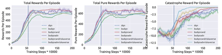
to specific dynamics and fail to transfer to other environments,   TABLE I: Robustness of Models Measured by Average Best
particularly those that involve random perturbations. We           Catastrophe Reward Per Episode (Higher is better)
denote this as dqn.                                                          Exp            Normal   Random Perturb   Adv. Perturb
   Ensemble DQN. Ensemble DQN tends to be more robust                        dqn             -0.80        -3.0            -4.0
                                                                            bsdqn            -0.90        -1.1            -2.5
than vanilla DQN. However, without being trained on different            bsdqnrand           -0.10        -1.0            -2.1
dynamics, even Ensemble DQN may not work well when                        bsdqnadv           -0.30        -0.5            -1.0
there are adversarial attacks or simple random changes in the        bsdqnrandriskaverse     -0.09        -0.4            -2.0
                                                                     bsdqnadvriskaverse      -0.08        -0.1            -0.1
dynamics. We denote this as bsdqn.
   Ensemble DQN with Random Perturbations Without
Risk Averse Term. We train the protagonist and provide             exploration rate decreases to 0.02 at 0.50 million steps, and
random perturbations according to the schedule Ξ. We do            we allow additional 50000 steps for learning to stabilize.
not include the variance guided exploration term here, so             Does adding adversarial agent’s perturbation affect the
only the Q value function is used for choosing actions. The        robustness? In Table I, we compare the robustness of all
schedule Ξ is the same as in our method. We denote this as         models by their catastrophe rewards. The results indicate
bsdqnrand.                                                         that adding perturbations improves a model’s robustness,
   Ensemble DQN with Random Perturbations With the                 especially to adversarial attacks. DQN trained with random
Risk Averse Term. We only train the protagonist agent and          perturbations is not as robust as models trained with adver-
provide random perturbations according to the adversarial          sarial perturbations, since random perturbations are weaker
training schedule Ξ. The protagonist selects action based on       than adversarial perturbations.
its Q value function and the risk averse term. We denote this         How does the risk term affect the robustness of the
as bsdqnrandriskaverse.                                            trained models? As shown in Figures 4 and 5, models
   Ensemble DQN with Adversarial Perturbation. This is             trained with the risk term achieved better robustness under
to compare our model with [11]. For a fair comparison, we          both random and adversarial perturbations. We attribute this
also use Ensemble DQN to train the policy while the variance       to the risk term encouraging the adversary to aggressively
term is not used as either risk-averse or risk-seeking term in     explore regions with high risk while encouraging the opposite
either agents. We denote this as bsdqnadv.                         for the protagonist.
   Our method. In our method, we train both the protagonist           How do adversarial perturbations compare to random
and the adversary with Ensemble DQN. We include here               perturbations? A trained adversarial agent can enforce
the variance guided exploration term, so the Q function and        stronger perturbations than random perturbations. By com-
its variance across different models will be used for action       paring Figure 4 and Figure 5, we see that the adversarial
selection. The adversarial perturbation is provided according      perturbation provides stronger attacks, which causes the
to the adversarial training schedule Ξ. We denote this as          reward to be lower than with random perturbations.
bsdqnadvriskaverse.                                                   We also visualize an example of the differences between
                                                                   a trained adversary and random perturbations in Figure 6,
C. Evaluation                                                      which shows that a trained adversary can force the protagonist
   To evaluate robustness of our trained models, we use            (a vanilla DQN model) to drive into a wall and crash.
the same trained models under different testing conditions,                                 V. C ONCLUSION
and evaluate using the previously-defined reward classes of
total progress (Equation 5), pure progress (Equation 6), and          We show that by introducing a notion of risk averse
additionally consider the reward of catastrophes. We present       behavior, a protagonist agent trained with a learned adversary
three broad sets of results: (1) No perturbations. (Figure 3)      experiences substantially fewer catastrophic events during
We tested all trained models from Section IV-B without             test-time rollouts as compared to agents trained without an
perturbations. (2) Random perturbations. (Figure 4) To             adversary. Furthermore, a trained adversarial agent is able
evaluate the robustness of trained models in the presence          to provide stronger perturbations than random perturbations
of random environment perturbations, we benchmarked all            and can provide a better training signal for the protagonist as
trained models using random perturbations. For every 10            compared to providing random perturbations. In future work,
actions taken by the main agent, 1 was taken at random. (3)        we will apply RARARL in other safety-critical domains, such
Adversarial Perturbations. (Figure 5) To test the ability of       as in surgical robotics.
our models to avoid catastrophes, which normally require                                   ACKNOWLEDGMENTS
deliberate, non-random perturbations, we test with a trained         Xinlei Pan is supported by Berkeley Deep Drive. Daniel Seita is
adversarial agent which took 1 action for every 10 taken by        supported by a National Physical Science Consortium Fellowship.
the protagonist.
   All subplots in Figures 3, 4, and 5 include a vertical blue
line at 0.55 million steps indicating when perturbations were
first applied during training (if any). Before 0.55 million
steps, we allow enough time for protagonist agents to be able
to drive normally. We choose 0.55 million steps because the
Fig. 3: Testing all models without attacks or perturbations. The reward is divided into distance related reward (left subplot), progress related reward (middle
subplot). We also present results for catastrophe reward per episode (right subplot). The blue vertical line indicates the beginning of adding perturbations
during training. All legends follow the naming convention described in Section IV-B.
Fig. 4: Testing all models with random attacks. The three subplots follow the same convention as in Figure 3.
Fig. 5: Testing all models with adversarial attack. The three subplots follow the same convention as in Figure 3.
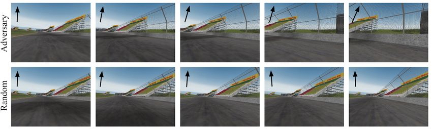
Fig. 6: Two representative (subsampled) sequences of states in TORCS for a trained protagonist, with either a trained adversary (top row) or random
perturbations (bottom row) affecting the trajectory. The overlaid arrows in the upper left corners indicate the direction of the vehicle. The top row indicates
that the trained adversary is able to force the protagonist to drive towards the right and into the wall (i.e., a catastrophe). Random perturbations cannot
affect the protagonist’s trajectory to the same extent because many steps of deliberate actions in one direction are needed to force a crash.R EFERENCES [23] Y. Chow, M. Ghavamzadeh, L. Janson, and M. Pavone, “Risk-
constrained reinforcement learning with percentile risk criteria,” Journal
[1] D. Silver, A. Huang, C. J. Maddison, A. Guez, L. Sifre, G. Van of Machine Learning Research, 2018.
Den Driessche, J. Schrittwieser, I. Antonoglou, V. Panneershelvam, [24] T. M. Moldovan and P. Abbeel, “Safe exploration in markov decision
M. Lanctot, et al., “Mastering the game of go with deep neural networks processes,” in International Conference on Machine Learning (ICML),
and tree search,” Nature, vol. 529, no. 7587, pp. 484–489, 2016. 2012.
[2] V. Mnih, K. Kavukcuoglu, D. Silver, A. A. Rusu, J. Veness, M. G. [25] J. Achiam, D. Held, A. Tamar, and P. Abbeel, “Constrained policy
Bellemare, A. Graves, M. Riedmiller, A. K. Fidjeland, G. Ostrovski, optimization,” in International Conference on Machine Learning
et al., “Human-level control through deep reinforcement learning,” (ICML), 2017.
Nature, vol. 518, no. 7540, pp. 529–533, 2015. [26] D. Held, Z. McCarthy, M. Zhang, F. Shentu, and P. Abbeel, “Proba-
bilistically safe policy transfer,” in IEEE International Conference on
[3] S. Shalev-Shwartz, S. Shammah, and A. Shashua, “Safe, multi-
Robotics and Automation (ICRA), 2017.
agent, reinforcement learning for autonomous driving,” arXiv preprint
[27] M. Plappert, R. Houthooft, P. Dhariwal, S. Sidor, R. Y. Chen, X. Chen,
arXiv:1610.03295, 2016.
T. Asfour, P. Abbeel, and M. Andrychowicz, “Parameter space noise for
[4] Y. You, X. Pan, Z. Wang, and C. Lu, “Virtual to real reinforcement
exploration,” in International Conference on Learning Representations
learning for autonomous driving,” British Machine Vision Conference,
(ICLR), 2018.
2017.
[28] M. Fortunato, M. G. Azar, B. Piot, J. Menick, I. Osband, A. Graves,
[5] T. P. Lillicrap, J. J. Hunt, A. Pritzel, N. Heess, T. Erez, Y. Tassa, V. Mnih, R. Munos, D. Hassabis, O. Pietquin, C. Blundell, and S. Legg,
D. Silver, and D. Wierstra, “Continuous control with deep reinforcement “Noisy networks for exploration,” in International Conference on
learning,” in International Conference on Learning Representations Learning Representations (ICLR), 2018.
(ICLR), 2016. [29] A. Rajeswaran, S. Ghotra, B. Ravindran, and S. Levine, “Epopt:
[6] Y. Duan, X. Chen, R. Houthooft, J. Schulman, and P. Abbeel, Learning robust neural network policies using model ensembles,” in
“Benchmarking deep reinforcement learning for continuous control,” in International Conference on Learning Representations (ICLR), 2017.
International Conference on Machine Learning (ICML), 2016. [30] B. Eysenbach, S. Gu, J. Ibarz, and S. Levine, “Leave no trace:
[7] J. Schulman, S. Levine, P. Moritz, M. I. Jordan, and P. Abbeel, “Trust Learning to reset for safe and autonomous reinforcement learning,” in
region policy optimization,” in International Conference on Machine International Conference on Learning Representations (ICLR), 2018.
Learning (ICML), 2015. [31] D. Gandhi, L. Pinto, and A. Gupta, “Learning to fly by crashing,” in
[8] Y. Zhu, Z. Wang, J. Merel, A. Rusu, T. Erez, S. Cabi, S. Tunya- IEEE/RSJ International Conference on Intelligent Robots and Systems
suvunakool, J. Kramar, R. Hadsell, N. de Freitas, and N. Heess, (IROS), 2017.
“Reinforcement and imitation learning for diverse visuomotor skills,” [32] A. Aswani, H. Gonzalez, S. S. Sastry, and C. Tomlin, “Provably safe and
in Robotics: Science and Systems (RSS), 2018. robust learning-based model predictive control,” Automatica, vol. 49,
[9] A. Nagabandi, G. Kahn, R. S. Fearing, and S. Levine, “Neural network no. 5, pp. 1216–1226, 2013.
dynamics for model-based deep reinforcement learning with model- [33] A. Aswani, P. Bouffard, and C. Tomlin, “Extensions of learning-
free fine-tuning,” in IEEE International Conference on Robotics and based model predictive control for real-time application to a quadrotor
Automation (ICRA), 2018. helicopter,” in American Control Conference (ACC), 2012. IEEE,
[10] F. Sadeghi and S. Levine, “CAD2RL: real single-image flight without 2012, pp. 4661–4666.
a single real image,” in Robotics: Science and Systems, 2017. [34] D. Pathak, P. Agrawal, A. A. Efros, and T. Darrell, “Curiosity-driven
[11] L. Pinto, J. Davidson, R. Sukthankar, and A. Gupta, “Robust adversarial exploration by self-supervised prediction,” in International Conference
reinforcement learning,” International Conference on Machine Learning on Machine Learning (ICML), vol. 2017, 2017.
(ICML), 2017. [35] M. Bellemare, S. Srinivasan, G. Ostrovski, T. Schaul, D. Saxton, and
[12] A. Mandlekar, Y. Zhu, A. Garg, L. Fei-Fei, and S. Savarese, “Adversar- R. Munos, “Unifying count-based exploration and intrinsic motivation,”
ially robust policy learning: Active construction of physically-plausible in Advances in Neural Information Processing Systems, 2016, pp.
perturbations,” in IEEE/RSJ International Conference on Intelligent 1471–1479.
Robots and Systems (IROS), 2017. [36] J. Tobin, R. Fong, A. Ray, J. Schneider, W. Zaremba, and P. Abbeel,
[13] A. Tamar, D. Di Castro, and S. Mannor, “Learning the variance of the “Domain randomization for transferring deep neural networks from
reward-to-go,” Journal of Machine Learning Research, vol. 17, no. 13, simulation to the real world,” in IEEE/RSJ International Conference
pp. 1–36, 2016. on Intelligent Robots and Systems (IROS), 2017.
[14] I. Osband, C. Blundell, A. Pritzel, and B. Van Roy, “Deep exploration [37] X. B. Peng, M. Andrychowicz, W. Zaremba, and P. Abbeel, “Sim-to-
via bootstrapped dqn,” in Advances in Neural Information Processing real transfer of robotic control with dynamics randomization,” in IEEE
Systems, 2016, pp. 4026–4034. International Conference on Robotics and Automation (ICRA), 2018.
[15] B. Wymann, E. Espié, C. Guionneau, C. Dimitrakakis, R. Coulom, and [38] G.-H. Liu, A. Siravuru, S. Prabhakar, M. Veloso, and G. Kantor,
A. Sumner, “Torcs, the open racing car simulator,” Software available “Learning end-to-end multimodal sensor policies for autonomous
at http://torcs. sourceforge. net, 2000. navigation,” in Conference on Robot Learning (CoRL), 2017.
[16] L. Pinto, J. Davidson, and A. Gupta, “Supervision via competition: [39] S. Ebrahimi, A. Rohrbach, and T. Darrell, “Gradient-free policy
Robot adversaries for learning tasks,” in IEEE International Conference architecture search and adaptation,” in Conference on Robot Learning
on Robotics and Automation (ICRA), 2017. (CoRL), 2017.
[17] T. Bansal, J. Pachocki, S. Sidor, I. Sutskever, and I. Mordatch, [40] A. Amini, L. Paull, T. Balch, S. Karaman, and D. Rus, “Learning
“Emergent complexity via multi-agent competition,” in International steering bounds for parallel autonomous systems,” in IEEE International
Conference on Learning Representations (ICLR), 2018. Conference on Robotics and Automation (ICRA), 2018.
[18] A. Pattanaik, Z. Tang, S. Liu, G. Bommannan, and G. Chowdhary, [41] D. P. Kingma and J. Ba, “Adam: A method for stochastic optimization,”
“Robust deep reinforcement learning with adversarial attacks,” arXiv in International Conference on Learning Representations (ICLR), 2015.
preprint arXiv:1712.03632, 2017.
[19] I. J. Goodfellow, J. Shlens, and C. Szegedy, “Explaining and harness-
ing adversarial examples,” in International Conference on Learning
Representations (ICLR), 2015.
[20] S. Paul, K. Chatzilygeroudis, K. Ciosek, J.-B. Mouret, M. A. Osborne,
and S. Whiteson, “Alternating optimisation and quadrature for robust
control,” in AAAI 2018-The Thirty-Second AAAI Conference on
Artificial Intelligence, 2018.
[21] R. Neuneier and O. Mihatsch, “Risk sensitive reinforcement learning,”
in Neural Information Processing Systems (NIPS), 1998.
[22] S. Carpin, Y.-L. Chow, and M. Pavone, “Risk aversion in finite markov
decision processes using total cost criteria and average value at risk,”
in IEEE International Conference on Robotics and Automation (ICRA),
2016.You can also read