Rolling Bearing Fault Diagnosis Based on Component Screening Vector Local Characteristic-Scale Decomposition
←
→
Page content transcription
If your browser does not render page correctly, please read the page content below
Hindawi
Shock and Vibration
Volume 2022, Article ID 9925681, 13 pages
https://doi.org/10.1155/2022/9925681

Research Article
Rolling Bearing Fault Diagnosis Based on Component Screening
Vector Local Characteristic-Scale Decomposition

 Tengfei Guan , Shijun Liu, Wenbo Xu, Zhisheng Li, Hongtao Huang, and Qi Wang
 Zhengzhou Research Institute of Mechanical Engineering Co., Ltd, Zhengzhou 45000, China

 Correspondence should be addressed to Tengfei Guan; guantengfei1314@126.com

 Received 9 April 2021; Revised 1 June 2021; Accepted 23 December 2021; Published 10 January 2022

 Academic Editor: Ke Feng

 Copyright © 2022 Tengfei Guan et al. This is an open access article distributed under the Creative Commons Attribution License,
 which permits unrestricted use, distribution, and reproduction in any medium, provided the original work is properly cited.

 The fault vibration signal of a bearing has nonstationary and nonlinear characteristics and can be regarded as the combination of
 multiple amplitude- and frequency-modulation components. The envelope of a single component contains the fault charac-
 teristics of a bearing. Local characteristic-scale decomposition (LCD) can decompose the vibration signal into a series of multiple
 intrinsic scale components. Some components can clearly reflect the running state of a bearing, and fault diagnosis is conducted
 according to the envelope spectrum. However, the conventional LCD takes a single-channel signal as the research object, which
 cannot fully reflect the characteristic information of the rotor, and the analysis results based on different channel signals of the
 same section will be inconsistent. To solve this problem, based on full vector spectrum technology, the homologous dual-channel
 information is fused. A vector LCD method based on cross-correlation coefficient component selection is given, and a simulation
 analysis is completed. The effectiveness of the proposed method is verified by simulated signals and experimental signals of a
 bearing, which provides a method for bearing feature extraction and fault diagnosis.

1. Introduction have been adopted to process nonstationary and nonlinear
 vibration signals. Among them, signal decomposition
Rotating machinery is developing in the direction of high methods contribute much. Tiwari [15] described a self-
speeds, heavy loads, and high reliability, which places higher adaptive signal decomposition technique, concealed com-
requirements on mechanical transmission equipment [1]. ponent decomposition (CCD), as the basis of a precise
The operational state of mechanical equipment is changing, bearing fault diagnosis model. Ying [16] introduced a novel
and its safe, stable, and reliable operation must be ensured. permutation entropy-based improved uniform phase em-
Rolling bearings are widely used in mechanical equipment, pirical mode decomposition (PEUPEMD) method and
and their working condition greatly affects its operation [2]. obtained better analysis than comparative methods about
Owing to complex operating conditions and changing ex- empirical mode decomposition (EMD) in decomposing
ternal environment, rolling bearings are prone to failure [3]. accuracy and mode mixing suppression. Patel [17] applied
It is of great significance to monitor their working status and variational mode decomposition (VMD) to filter out non-
diagnose their fault degree [4, 5]. Some studies have focused stationarities due to variable speed conditions and provided
on the fault features of rotating machinery through modern a complete diagnostic solution for the spur gear systems. Li
signal processing methods [6–8]. [18] presented a local mean decomposition (LMD) method
 Fault vibration signals of bearings are usually weak based on an improved compound interpolation envelope,
nonstationary signals with complex frequency components. whose effect was comparable to or slightly better than that of
The key to fault diagnosis of rolling bearings is to extract other methods. Zheng [19] proposed local characteristic-
effective feature information from vibration signals con- scale decomposition (LCD), a nonstationary signal analysis
taining complex frequencies [9]. Vibration analysis and fault method that adaptively decomposes a signal to a series of
diagnosis have received considerable attention [10–14] and intrinsic scale components in different scales. With good
2 Shock and Vibration

compatibility, LCD methods have seen new applications, from a test stand by a signal acquisition module. Then, the
such as the local characteristic-scale decomposition-Teager vector LCD method was used to compute and analyze the
energy operator (LCD-TEO) [20], improved local charac- data. Next, the fusion data were enveloped into the
teristic-scale decomposition (ILCD) [21], and piecewise spectrum. Lastly, the fault frequency features were
cubic Hermite interpolating polynomial-local characteristic- matched with the specific fault type and the failure reason
scale decomposition (PCHIP-LCD) [22]. was located.
 However, the conventional LCD methods focus on single-
channel signals, which probably cause incomplete fault fea-
ture extraction. In the fault diagnosis of rotating machinery, 2.1. Local Characteristic-Scale Decomposition. According to
the sensor information collected by a multi-sensor system is the extreme value of a signal, the LCD can adaptively de-
related to the same or different sides of rotating machinery in compose nonlinear and nonstationary signals to a series of
the same environment. There is an inevitable connection ISCs satisfying the following conditions:
between various types of information, which are different in (1) The length between any two adjacent extreme points
time, space, credibility, and expression, whose focuses and of the data sample is monotonic
uses are not exactly the same, and whose requirements for
information processing and management are different. If the (2) If the extreme point in a data sample is Xk (k � 1, 2,
information collected by each source is considered in isola- ..., M) and τ k is the corresponding time, then any two
tion, then their internal connections and characteristics are maximum (or minimum) value points (τ k , Xk ),
lost. Multi-source information fusion can solve this problem (τ k+2 , Xk+2 ) can be connected to form a line segment.
[23]. Multi-sensor data fusion methodologies include the τ k+1 is the corresponding time of the maximum (or
holospectrum [24–27], full spectrum [28–31], and full vector minimum) value point (τ k+1 , Xk+1 ) in the middle of
spectrum [32]. Proposed by Han [32], the full vector spectrum the line segment. The corresponding function value
has been widely studied and applied in engineering [33–35] at this moment is
and has formed the basis of many compound methods. Chen
[36] applied full-vector signal acquisition and information τ k+1 − τ k
fusion to fault prediction. Gong [37] combined the full vector Ak � Xk + X − Xk . (1)
 τ k+2 − τ k k+2
spectrum with ensemble empirical decomposition and ap-
plied it to the diagnosis of gear faults. Yu [38] introduced the The ratio of the function value to the maximum (or
empirical wavelet transform and variance contribution rate to minimum)
the full vector spectrum, which improved the adaptability and
accuracy of full vector information fusion. τ k+1 − τ k
 a X k + X − Xk +(1 − a)Xk+1 � 0, (2)
 Based on the above analysis, the main contributions of τ k+2 − τ k k+2
this paper are as follows:
 remains unchanged, where a ∈ (0, 1) is a constant, and
 (1) A signal processing method, vector LCD, is pro- a � 1/2 for frequency modulated, amplitude modulated,
 posed, which fully considers homologous signals and amplitude-frequency modulated, and sine-cosine signals.
 intrinsic scale components (ISCs) On the basis of the ISC, LCD can decompose any signal
 (2) Vector LCD can simplify the analysis of ISCs by taking x(t) to a series of ISCs, as follows [39]:
 the cross-correlation coefficient in screening components (1) Find all extreme points of x(t) and their corre-
 (3) The fusion of optimal components can obtain more sponding moments τ k (k � 1, 2, ..., M), set a � 1/2,
 complete and accurate fault features and make a linear transformation for x(t) between
 any two extreme points,
 The remainder of this article is arranged as follows.
Section 2 shows the calculation of LCD, presents the theory Lk+1 − Lk
of the cross-correlation coefficient, describes the principles P1 � L k + x − Xk ,
 Xk+1 − Xk t
of the conventional full vector spectrum, and introduces a
method for bearing feature extraction and fault diagnosis τ k+1 − τ k
based on the correlation coefficient vector LCD. In Section 3, Lk+1 � a Xk + X − Xk +(1 − a)Xk+1 ,
 τ k+2 − τ k k+2
the proposed methodology is verified through application to
the homologous simulation signals of a rolling bearing. In (3)
Section 4, the rolling bearing experimental data from two
directions of sensors are used to validate vector LCD. where t ∈ (τ k , τ k+1 ).
Conclusions are given in Section 5. (2) Subtract P1 (t) from the original signal x(t) to get a
 new signal,

2. Theoretical Description of Vector LCD I1 (t) � x(t) − P1 (t). (4)

The proposed fault diagnosis method using vector local (3) Ideally, I1 (t) can be used as the first ISC. At this
characteristic-scale decomposition (Vector LCD) is moment Lk+1 is equal to zero; in practice, assuming a
presented in Figure 1. Vibration signals were obtained variable △e, the iteration ends when |Lk+1 | ≤ △e. If
Shock and Vibration 3

 Signal acquisition
 module

 A test stand

 X signal Y signal Vibration signals

 Vector LCD

 Envelop spectrum

 Fault frequency
 matching

 Fault diagnosis

 Figure 1: Block diagram of the proposed fault diagnosis method using vector LCD.

 I1 (t) does not meet the two conditions of ISC, the ni�1 xi − x yi − y
 above steps are repeated k times until Ik (t) satisfies r � ����������� � , (6)
 2 2
 the conditions and denote Ik (t) as the first ISC c1 (t) ni�1 xi − x ni�1 yi − y
 of x(t).
 (4) Subtract c1 (t) from x(t) to get a new signal, r1 . Take where x and y are the mean values of sequences x-and y,
 r1 as the original data and repeat steps 1–3 to get the respectively.
 second ISC component, c2 (t), of x(t). Repeat n times Suppose xnor and ynor are normal operating signals
 to get n ISCs of the signal x(t). The function does not perpendicular to each other, and xabn , yabn are the homol-
 terminate until rn is monotonic: ogous signals when faults occur. After the decomposition of
 n LCD, we obtain four ISCs, ISCxnork , ISCynork , ISCyabnk , and
 x(t) � cp (t) + rn (t). (5) ISCxabnk , where k � 1, 2, . . ., N is the order of an ISC. The
 p�1 cross-correlation coefficient is calculated as follows:
 (1) Calculate the correlation coefficients between
 It can be seen from equation (5) that the signal x(t) can ISCxnork and xnor , ISCynork , and ynor , and find their
be reconstructed by n ISCs and a monotonic signal. average, Uk ;
 (2) Calculate the correlation coefficients between
 ISCxabnk and xabn , ISCyabnk , and ISCyabnk , and find
2.2. Correlation Coefficient. Correlation is a kind of non-
 their average, Vk ;
deterministic relationship, and the correlation coefficient
measures the degree of linear correlation between variables. (3) Calculate the correlation coefficients between
The correlation coefficient between sequences ISCxnork and ISCynork , ISCxabnk , and ISCyabnk , and find
x � (x1 , x2 , . . . , xn ) and y � (y1 , y2 , . . . , yn ) can be calcu- their average, Wk ;
lated as (4) Calculate the sensitivity factor,
4 Shock and Vibration

 U k + Vk next optimal ISC of orthogonal signals can be obtained, the
 Sk � − Wk , (7) vector ISCs are formed through the optimal ISC component
 2
 fusion, and the vector ISCs are enveloped and demodulated.
where Uk and Vk indicate the degree of correlation between The proposed method can identify the nonlinear charac-
the decomposed ISC and the initial signal. The larger the teristics of fault signals for fault diagnosis.
value, the more similar are ISC and the initial signal. The Wk
indicates the correlation between ISCs of the same order. 3. Simulation Analysis
The smaller the value, the greater the change in the ISC.
Overall, the larger the Sk , the more sensitive the ISC of this Analog signals were analyzed to validate the effectiveness of
order, and the more it can reflect spectral changes. vector local characteristic-scale decomposition in processing
 homologous signals. For the rolling bearing signal, the vi-
2.3. Full Vector Spectrum. To overcome limitations due to bration signal at the time of failure presents a modulation
incomplete and inaccurate sensor information, two or- phenomenon. The vibration signal of a rolling bearing with
thogonal sensors are usually fixed on the same section of the an outer ring fixed structure is
rotor in the field test of large rotating machinery. The full x(t) � α sin 2πfb 1 + β sin 2πfr t , (9)
vector spectrum technology meets the accuracy and reli-
ability requirements of condition monitoring and fault di- where fb is the passing frequency of the inner ring of the
agnosis. The vortex phenomenon of the rotor is the rolling bearing and fr is the rotation frequency of the rotor.
combined effect of each harmonic frequency, and the vortex Based on this, the following analog acceleration signal is
intensity at each harmonic frequency is the basis for fault constructed:
judgment and identification. The space rotation trajectory of
 ⎧
 ⎪
 ⎪ xnor (t) � sin(40πt) + sin(600πt),
each harmonic is an ellipse, and the maximum vibration ⎪
 ⎪
vector is in its long-axis direction [40]. ⎪
 ⎪ ynor (t) � cos(40πt) + cos(600πt),
 ⎪
 ⎪
 Suppose the cross section channel signals ( xk and yk ) ⎪
 ⎪
 ⎪
 ⎨ xabn (t) � sin(40πt) + 0.8 sin(600πt) + 0.9(1 + sin(40πt))
are perpendicular to each other and form them into a ⎪ sin(200πt),
complex signal ( zk � xk + j yk ), only a single Fourier ⎪
 ⎪
 ⎪
 ⎪
transform (FT) of the complex signal is needed to obtain the ⎪
 ⎪
 ⎪
 ⎪ yabn (t) � cos(40πt) + 1.2 cos(600πt) +(1 + sin(40πt))
characteristic information required by the full vector ⎪
 ⎪
 ⎩
spectrum under each harmonic frequency. The algorithm is cos(200πt),
robust, it greatly reduces calculation, and it is compatible (10)
with conventional analysis methods. When processing a
single-channel signal, the algorithm is still valid and can where xnor (t) and ynor (t) are two initial vibration signals
meet real-time requirements. The characteristic information that are perpendicular to each other under normal operating
includes the main vibration vector RLk , assistant vibration conditions, xabn (t) and yabn (t) are two initial vibration
vector Rsk , angle ∅αk between the main vibration vector and signals that are perpendicular to each other under abnormal
the x-axis, and the elliptical trajectory’s initial phase angle αk , operating conditions, the sampling frequency fs � 1024Hz,
which are described by and there are N � 2048 sampling points.
 The LCD is applied to decompose the two-channel
 ⎪
 ⎧ 1 signals corresponding to normal operating conditions. The
 ⎪
 ⎪ RLk � Zk + ZN−k ,
 ⎪
 ⎪ 2N time-domain waveforms and the ISCs are shown in Figure 3
 ⎪
 ⎪
 ⎪
 ⎪ for x-channel signals and Figure 4 for y-channel signals.
 ⎪
 ⎪
 ⎪
 ⎪ 1 The LCD is then applied to decompose the two-channel
 ⎪
 ⎪ Rsk � Zk − ZN−k ,
 ⎪
 ⎪ 2N signals corresponding to abnormal operating conditions, for
 ⎪
 ⎪
 ⎨ which the time-domain waveforms and the ISCs of x- and
 ⎪ (8) y-channel signals are shown in Figures 5 and 6, respectively.
 ⎪
 ⎪ ZIk ZR(N−k) − ZRk ZI(N−k)
 ⎪
 ⎪ tan 2∅αk � , The correlation coefficients between ISCs and initial
 ⎪
 ⎪ ZIk ZI(N−k) + ZRk ZR(N−k)
 ⎪
 ⎪ signals can be calculated, i.e., between ISCxnori and xnor,
 ⎪
 ⎪
 ⎪
 ⎪ ISCynori and ynor, ISCxabni and xabn, and ISCyabni and yabn, as
 ⎪
 ⎪
 ⎪
 ⎪ ZIk + ZI(N−k) shown in Table 1.
 ⎪
 ⎪
 ⎩ tan αk � , Figures 5 and 6 show that the initial signals are
 ZRk + ZR(N−k)
 decomposed to six ISCs with different frequency bands.
where k � 1, 2, . . ., N/2–1. The characteristic information of There is a great difference in amplitude between the x- and
each harmonic trace from equation (8) is the main char- y-directions. If the signal is analyzed in a certain direction
acteristic information under each harmonic trace of full alone, the analysis results will also be quite different.
vector spectrum technology. Therefore, information fusion is necessary. The full vector
 Figure 2 is a flowchart of the proposed method. At first, fusion is introduced. Considering the value of the correla-
the LCD is applied to the homology information acquired tion coefficient, the first-order ISCxnor and third-order
from two orthogonal sensors. The cross-correlation coeffi- ISCynor are closer to the initial signals than the others. The
cient is selected to choose the ISCs of orthogonal signals, the second-order ISCxabn and second-order ISCyabn have more
Shock and Vibration 5

 x direction sensor y direction sensor

 {xk} {yk}

 LCD LCD

 component ISCxi ISCyi component
 screening screening

 optimal component optimal component
 ISCxo ISCyo

 full vector fusion

 ISCzo

 envelope &
 demodulation analysis

 fault diagnosis

 Figure 2: Flowchart of vector LCD.

 4 2
 2
 ISC1
 xnor

 0 0
 -2
 -4 -2
 0 0.2 0.4 0.6 0.8 1 0 0.2 0.4 0.6 0.8 1
 2 2
 ISC2

 ISC3

 0 0
 Amplitude (g)

 Amplitude (g)

 -2 -2
 0 0.2 0.4 0.6 0.8 1 0 0.2 0.4 0.6 0.8 1
 2 2
 ISC4

 ISC5

 0 0

 -2 -2
 0 0.2 0.4 0.6 0.8 1 0 0.2 0.4 0.6 0.8 1
 2 2
 ISC6

 res.

 0 0

 -2 -2
 0 0.2 0.4 0.6 0.8 1 0 0.2 0.4 0.6 0.8 1
 Time (s) Time (s)
 Figure 3: LCD decomposition results of x-channel under normal conditions.
6 Shock and Vibration 4 2 2 ISC1 ynor 0 0 -2 -4 -2 0 0.2 0.4 0.6 0.8 1 0 0.2 0.4 0.6 0.8 1 2 2 ISC2 ISC3 0 0 Amplitude (g) Amplitude (g) -2 -2 0 0.2 0.4 0.6 0.8 1 0 0.2 0.4 0.6 0.8 1 2 2 ISC4 ISC5 0 0 -2 -2 0 0.2 0.4 0.6 0.8 1 0 0.2 0.4 0.6 0.8 1 2 2 ISC6 0 res. 0 -2 -2 0 0.2 0.4 0.6 0.8 1 0 0.2 0.4 0.6 0.8 1 Time (s) Time (s) Figure 4: LCD decomposition results of y-channel under normal conditions. 4 2 2 ISC1 xabn 0 0 -2 -4 -2 0 0.2 0.4 0.6 0.8 1 0 0.2 0.4 0.6 0.8 1 2 2 ISC2 ISC3 0 0 Amplitude (g) Amplitude (g) -2 -2 0 0.2 0.4 0.6 0.8 1 0 0.2 0.4 0.6 0.8 1 2 2 ISC4 ISC5 0 0 -2 -2 0 0.2 0.4 0.6 0.8 1 0 0.2 0.4 0.6 0.8 1 2 2 ISC6 res. 0 0 -2 -2 0 0.2 0.4 0.6 0.8 1 0 0.2 0.4 0.6 0.8 1 Time (s) Time (s) Figure 5: LCD decomposition results of x-channel under abnormal conditions.
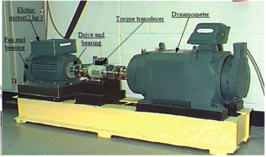
Shock and Vibration 7

 4 2
 2

 ISC1
 yabn
 0 0
 -2
 -4 -2
 0 0.2 0.4 0.6 0.8 1 0 0.2 0.4 0.6 0.8 1
 2 2
 ISC2

 ISC3
 0 0
 Amplitude (g)

 Amplitude (g)
 -2 -2
 0 0.2 0.4 0.6 0.8 1 0 0.2 0.4 0.6 0.8 1
 2 2
 ISC4

 ISC5
 0 0

 -2 -2
 0 0.2 0.4 0.6 0.8 1 0 0.2 0.4 0.6 0.8 1
 2 2
 ISC6

 0 res. 0

 -2 -2
 0 0.2 0.4 0.6 0.8 1 0 0.2 0.4 0.6 0.8 1
 Time (s) Time (s)
 Figure 6: LCD decomposition results of y-channel under abnormal conditions.

 Table 1: Correlation coefficients of ISCs of each order between two channel signals under two conditions.
ISC order 1 2 3 4 5 6
 xnor 0.7035 0.1648 0.6998 0.0869 0.0032 0.0062
 ynor 0.6983 0.1851 0.7045 −0.1065 0.11 −0.0203
Correlation coefficient
 xabn 0.5308 0.6293 0.4658 0.6119 0.0043 −0.0628
 yabn 0.6385 0.6576 0.5345 0.0147 −0.0027 0.0125
The bold value is the maximum value of all ISCs (between the order 1 to 6).

fault information than others. Thus, we apply full vector 4. Application
fusion to the first-order ISCxnor, third-order ISCynor, second-
order ISCxabn, and second-order ISCyabn. However, the fault The validity and advantage of vector LCD in fault diagnosis
frequency information cannot be acquired just from time- of a rolling bearing were examined through experimental
domain waveforms. Finally, envelope and demodulation are data from the Case Western Reserve University bearing data
applied to fusion signals, as shown in Figure 7. It is clear in center. Figure 8 shows the layout of the test stand, which
Figure 7(a) that the rotation frequencies (20 Hz and 300 Hz) consisted of a 2-hp motor, torque transducer/encoder, dy-
are consistent with the preset value under the normal op- namometer, and control electronics. The test bearings
erating condition. In Figure 7(b), the amplitudes of the fault supported the motor shaft, and they had single-point faults
frequency (100 Hz) and sidebands (20 Hz) show the exis- from electro-discharge machining. Accelerometers collected
tence of modulation under the abnormal operating vibration data and were attached to the support of the drive
condition. end bearing, fan end bearing, and motor supporting base.
 From the simulation analysis, the vector LCD has a good The technical parameters of fault diagnosis are listed in
analysis result when applied to fault signals with frequency Table 2.
or amplitude modulation, which can enhance the accuracy Normal baseline data, outer race fault data, and inner
of fault diagnosis. The adoption of the cross-correlation race fault data were adopted from the experimental signals.
coefficient avoids repeated analysis between multiple com- The ball fault data frequency is not matched with the usual
ponents and simplifies the analysis, for a unique and ac- value for the slip adjusting to lock onto a dominant fre-
curate conclusion. quency [41]. Therefore, ball fault data are not discussed here.
8 Shock and Vibration

 2 2

 Amplitude (g)
 Amplitude (g)

 1.5 1.5
 (20,0.9775) (300,0.9953)
 1 1 (100,0.8894)

 0.5 0.5 (80,0.3499) (120,0.4096)

 0 0
 0 50 100 150 200 250 300 350 400 0 50 100 150 200 250 300 350 400
 Frequency (Hz) Frequency (Hz)
 (a) (b)

 Figure 7: Vector LCD spectra of simulation signals: (a) normal condition; (b) abnormal condition.

 Figure 8: Case Western Reserve University bearing test stand.

 Table 2: Technical parameters.
Fault location Fault diameter (inches) Fault depth (inches) Motor load (hp) Sampling frequency (Hz)
Normal 0 0 0 12000
Outer race 0.007 0.011 0 12000
Inner race 0.007 0.011 0 12000
Fault location Motor speed (rpm) Defect frequencies (Hz) Sample points Data file name
Normal 1797 — 8192 97.mat
Outer race 1797 107.3 8192 130.mat/144.mat
Inner race 1797 162.1 8192 105.mat

4.1. Normal Baseline Data Analysis. Because the normal analysis. Similar to normal baseline data processing, ISC
baseline data only have one channel of drive end section, components were acquired after LCD. The ISC components
processing the single-sensor data is just a special case of a full of the x-and y-channels are shown in Figures 11 and 12,
vector spectrum. According to the flowchart of vector LCD, respectively. As seen in Table 4, the first ISC components of
we first applied LCD to the drive-end single-channel signal the x-and y-signals are optimal. From Figures 11 and 12, the
to obtain 10 ISCs. Considering that the higher the order of time-domain waves of the first ISC components of the x- and
ISC, the smaller the amplitude, only the first six orders of y-signals have different amplitudes and frequencies. If only
ISCs are displayed in Figure 9. We compare the values of ISC one direction of the x- or y-signal is analyzed, then different
cross-correlation coefficients in Table 3, where the first is the results will be obtained, which is contrary to fault diagnosis.
optimal component. Finally, the envelope and demodulation Therefore, we apply full vector fusion to the two optimal ISC
are applied to the first ISC. From Figure 10, the rotation components to obtain a new combined signal. Finally, the
frequency fr (29.95 Hz) and 2fr (59.9 Hz) account for the envelope and demodulation are applied to the combined
main components without other fault frequencies, which is a signal. The outer race fault frequency fOR (107.3 Hz) can be
normal operating condition. easily distinguished from other spectra, and the amplitude of
 fOR is the highest among all spectra (as seen in Figure 13).
4.2. Outer Race Fault Data Analysis. Outer race fault data
were obtained by three homologous sensors in the same 4.3. Inner Race Fault Data Analysis. Inner race fault data were
section, and channels of centered 6 : 00 clock and or- recorded in a single channel for the drive end, and the inner
thogonal 3 : 00 clocks were employed to vector LCD race fault signal was treated in the same way as normal
Shock and Vibration 9

 0.5 0.2

 ISC1
 xnor
 0 0

 -0.5 -0.2
 0 0.2 0.4 0.6 0 0.2 0.4 0.6
 0.2 0.1
 ISC2

 ISC3
 0 0
 Amplitude (g)

 Amplitude (g)
 -0.2 -0.1
 0 0.2 0.4 0.6 0 0.2 0.4 0.6
 0.1 0.1
 ISC4

 ISC5
 0 0

 -0.1 -0.1
 0 0.2 0.4 0.6 0 0.2 0.4 0.6
 0.1 0.5
 ISC6

 0 res.

 -0.1 0
 0 0.2 0.4 0.6 0 0.2 0.4 0.6
 Time (s) Time (s)
 Figure 9: LCD decomposition results of x-channel under normal conditions.

 Table 3: Correlation coefficients of ISCs of each order under normal conditions.
ISC order 1 2 3 4 5
Correlation coefficient 0.7994 0.5678 0.3904 0.4009 0.3037
ISC order 6 7 8 9 10
Correlation coefficient 0.1167 0.0773 0.0052 0.0077 0.0042
The bold value is the maximum value of all ISCs (between the order 1 to 10).

 0.04 fr
 Amplitude (g)

 2fr
 0.02

 0
 0 100 200 300 400 500 600
 Frequency (Hz)
 Figure 10: Vector LCD spectra of x-channel under normal conditions.

baseline data. The vector LCD spectra can be displayed after This bearing experimental application shows that the
the optimal ISC is screened out, with decomposition results as proposed method can be applied to rolling bearing fault
shown in Figure 14. From Table 5, the optimal ISC (the first diagnosis. The screening of the optimal ISC can simplify
ISC component) can be easily obtained. From the vector LCD fault diagnosis and clearly display the typical features. The
spectra in Figure 15, the inner race fault frequency fIR full vector fusion between optimal ISCs of the x- and
(162.1 Hz) and rotation frequency harmonics fr (29.95 Hz), 2fr y-signals gives an accurate and unique conclusion for fault
(59.9 Hz), and 4fr (119.8 Hz) can be acquired from the spectra, diagnosis. The vector LCD provides an easy way to extract
which agrees with the inner race fault features. fault features.
10 Shock and Vibration

 0.5 0.2

 ISC1
 xOR
 0 0

 -0.5 -0.2
 0 0.2 0.4 0.6 0 0.2 0.4 0.6
 0.2 0.1
 ISC2

 ISC3
 0 0
 Amplitude (g)

 Amplitude (g)
 -0.2 -0.1
 0 0.2 0.4 0.6 0 0.2 0.4 0.6
 0.1 0.1
 ISC4

 ISC5
 0 0

 -0.1 -0.1
 0 0.2 0.4 0.6 0 0.2 0.4 0.6
 0.1 0.5
 ISC6

 0 res.

 -0.1 0
 0 0.2 0.4 0.6 0 0.2 0.4 0.6
 Time (s) Time (s)
 Figure 11: LCD decomposition results of x-channel under outer race fault condition.

 0.5 0.2
 ISC1
 yOR

 0 0

 -0.5 -0.2
 0 0.2 0.4 0.6 0 0.2 0.4 0.6
 0.2 0.1
 ISC2

 ISC3

 0 0
 Amplitude (g)

 Amplitude (g)

 -0.2 -0.1
 0 0.2 0.4 0.6 0 0.2 0.4 0.6
 0.1 0.1
 ISC4

 ISC5

 0 0

 -0.1 -0.1
 0 0.2 0.4 0.6 0 0.2 0.4 0.6
 0.1 0.5
 ISC6

 res.

 0

 -0.1 0
 0 0.2 0.4 0.6 0 0.2 0.4 0.6
 Time (s) Time (s)
 Figure 12: LCD decomposition results of y-channel under outer race fault condition.
Shock and Vibration 11

 Table 4: Correlation coefficient of ISCs of each order under outer race fault condition.
ISC order Direction 1 2 3 4 5 6
Correlation x 0.8375 0.5643 0.2833 0.2490 0.1737 0.1280
coefficient y 0.7529 0.6911 0.3957 0.2071 0.1321 0.0858
ISC order Direction 7 8 9 10 11 12
Correlation x 0.0712 0.0243 0.0089 0.0001 0.002 —
coefficient y 0.0426 −0.001 0.0054 0.0017 0.0004 0.0008

 0.03
 fOR
 Amplitude (g)

 0.02
 2fOR
 0.01

 0
 0 100 200 300 400 500 600
 Frequency (Hz)
 Figure 13: Vector LCD spectra of vector signal under outer race fault condition.

 0.5 0.2
 ISC1
 xIR

 0 0

 -0.5 -0.2
 0 0.2 0.4 0.6 0 0.2 0.4 0.6
 0.2 0.1
 ISC2

 ISC3

 0 0
 Amplitude (g)

 Amplitude (g)

 -0.2 -0.1
 0 0.2 0.4 0.6 0 0.2 0.4 0.6
 0.1 0.1
 ISC4

 ISC5

 0 0

 -0.1 -0.1
 0 0.2 0.4 0.6 0 0.2 0.4 0.6
 0.1 0.5
 ISC6

 res.

 0

 -0.1 0
 0 0.2 0.4 0.6 0 0.2 0.4 0.6
 Time (s) Time (s)
 Figure 14: LCD decomposition results of x-channel under inner race fault condition.

 Table 5: Correlation coefficient of ISCs of each order under inner race fault condition.
ISC order 1 2 3 4 5 6
Correlation coefficient 0.7563 0.7399 0.4803 0.3197 0.1993 0.1183
ISC order 7 8 9 10 11 12
Correlation coefficient 0.0300 0.0230 0.0005 0.0005 0.0013 0.0005
The bold value is the maximum value of all ISCs (between the order 1 to 12).
12 Shock and Vibration

 0.02 graphs,” Advanced Engineering Informatics, vol. 47, Article ID
 2fr 101253, 2021.
 Amplitude (g)

 0.015
 fr 4fr [4] J. Cheng, Y. Yang, X. Li, and J. Cheng, “Adaptive periodic
 0.01 fIR mode decomposition and its application in rolling bearing
 fault diagnosis,” Mechanical Systems and Signal Processing,
 0.005
 vol. 161, Article ID 107943, 2021.
 0 [5] W. Zhu, G. Ni, Y. Cao, and H. Wang, “Research on a rolling
 0 100 200 300 400 500 600
 bearing health monitoring algorithm oriented to industrial
 Frequency (Hz)
 big data,” Measurement, vol. 185, Article ID 110044, 2021.
Figure 15: Vector LCD spectra of x-signal under inner race fault [6] A. Glowacz, “Ventilation diagnosis of angle grinder using
condition. thermal imaging,” Sensors, vol. 21, no. 8, p. 2853, 2021.
 [7] P. Luo, N. Hu, L. Zhang, J. Shen, and Z. Cheng, “Improved
 phase space warping method for degradation tracking of
5. Conclusion rotating machinery under variable working conditions,”
 Mechanical Systems and Signal Processing, vol. 157, Article ID
A multiple signal processing method of rolling bearing fault 107696, 2021.
diagnosis was described in this paper. By combining the full [8] X. Li, Y. Yang, H. Shao, X. Zhong, J. Cheng, and J. Cheng,
vector spectrum with local characteristic-scale decomposi- “Symplectic weighted sparse support matrix machine for gear
tion, the vector LCD can fully consider homologous signals fault diagnosis,” Measurement, vol. 168, Article ID 108392,
and ISCs. This method is used to synchronously handle 2021.
multiple signals. The cross-correlation coefficient was in- [9] J. Yang, D. Huang, D. Zhou, and H. Liu, “Optimal IMF se-
troduced to choose ISCs, which simplifies the analysis of lection and unknown fault feature extraction for rolling
ISCs. The vector ISC displays a more complete and precise bearings with different defect modes,” Measurement, vol. 157,
fault frequency than a single ISC. The simulation analysis Article ID 107660, 2020.
and rolling bearing experimental fault diagnosis verified the [10] A. Klausen, H. V. Khang, and K. G. Robbersmyr, “Multi-band
effectiveness of vector LCD. With the good compatibility of identification for enhancing bearing fault detection in variable
 speed conditions,” Mechanical Systems and Signal Processing,
vector LCD, various types of faults and machines could be
 vol. 139, Article ID 106422, 2020.
diagnosed in our future work. Moreover, the signals from
 [11] Y. Ma, J. Cheng, P. Wang, J. Wang, and Y. Yang, “Rotating
different types of sensors will be combined to improve the machinery fault diagnosis based on multivariate multiscale
accuracy of fault diagnosis. fuzzy distribution entropy and Fisher score,” Measurement,
 vol. 179, Article ID 109495, 2021.
Data Availability [12] A. Glowacz, R. Tadeusiewicz, S. Legutko et al., “Fault diag-
 nosis of angle grinders and electric impact drills using acoustic
The experimental data were taken from the Case Western signals,” Applied Acoustics, vol. 179, Article ID 108070, 2021.
Reserve University bearing data center. [13] M. Hosseinpour-Zarnaq, M. Omid, and E. Biabani-Aghdam,
 “Fault Diagnosis of Tractor Auxiliary Gearbox Using Vi-
 bration Analysis and Random forest Classifier,” Information
Conflicts of Interest
 Processing in Agriculture, 2021, In press.
The authors declare that there are no conflicts of interest [14] H. Pan, H. Xu, J. Zheng, J. Su, and J. Tong, “Multi-class fuzzy
regarding the publication of this paper. support matrix machine for classification in roller bearing
 fault diagnosis,” Advanced Engineering Informatics, vol. 51,
 Article ID 101445, 2022.
Acknowledgments [15] P. Tiwari and S. H. Upadhyay, “Novel self-adaptive vibration
 signal analysis: concealed component decomposition and its
The authors would like to thank the National Key Research application in bearing fault diagnosis,” Journal of Sound and
and Development Program of China (2016YFF0203100) and Vibration, vol. 502, Article ID 116079, 2021.
the Henan Provincial Key Science and Technology Research [16] W. Ying, J. Zheng, H. Pan, and Q. Liu, “Permutation entropy-
Project of China (202102210075). The authors also thank the based improved uniform phase empirical mode decomposi-
Case Western Reserve University bearing data center for the tion for mechanical fault diagnosis,” Digital Signal Processing,
bearing fault test data. vol. 117, Article ID 103167, 2021.
 [17] A. Patel and P. Shakya, “Spur gear crack modelling and
 analysis under variable speed conditions using variational
References
 mode decomposition,” Mechanism and Machine Theory,
 [1] R. Liu, B. Yang, E. Zio, and X. Chen, “Artificial intelligence for vol. 164, Article ID 104357, 2021.
 fault diagnosis of rotating machinery: a review,” Mechanical [18] X. Li, J. Ma, X. Wang, J. Wu, and Z. Li, “An improved local
 Systems and Signal Processing, vol. 108, pp. 33–47, 2018. mean decomposition method based on improved composite
 [2] B. Zhao, X. Zhang, H. Li, and Z. Yang, “Intelligent fault interpolation envelope and its application in bearing fault
 diagnosis of rolling bearings based on normalized CNN feature extraction,” ISA Transactions, vol. 97, pp. 365–383,
 considering data imbalance and variable working conditions,” 2020.
 Knowledge-Based Systems, vol. 199, Article ID 105971, 2020. [19] J. Zheng, J. Cheng, and Y. Yang, “A rolling bearing fault
 [3] Y. Gao and D. Yu, “Intelligent fault diagnosis for rolling diagnosis approach based on LCD and fuzzy entropy,”
 bearings based on graph shift regularization with directed Mechanism and Machine Theory, vol. 70, pp. 441–453, 2013.
Shock and Vibration 13

[20] H. Liu, X. Wang, and C. Lu, “Rolling bearing fault diagnosis [38] H. Yu, H. Li, Y. Li, and Y. Li, “A novel improved full vector
 based on LCD-TEO and multifractal detrended fluctuation spectrum algorithm and its application in multi-sensor data
 analysis,” Mechanical Systems and Signal Processing, vol. 60- fusion for hydraulic pumps,” Measurement, vol. 133,
 61, pp. 273–288, 2015. pp. 145–161, 2019.
[21] L. Wang and Z. Liu, “An improved local characteristic-scale [39] J. Cheng, J. Zheng, and Y. Yang, “A new non-stationary signal
 decomposition to restrict end effects, mode mixing and its analysis approach-the local characteristic-scale decomposi-
 application to extract incipient bearing fault signal,” Me- tion method,” Journal of Vibration Engineering, vol. 25, no. 2,
 chanical Systems and Signal Processing, vol. 156, Article ID pp. 215–220, 2012.
 107657, 2021. [40] J. Han and L. Shi, “Study on space precession and vibration
[22] C. Yang, J. Ma, X. Wang, X. Li, Z. Li, and T. Luo, “A Novel characteristic of high-speed rotary shaft,” Journal of Vibration
 Based-Performance Degradation Indicator RUL Prediction Engineering, vol. 17, no. 3, pp. 69–72, 2004.
 Model and its Application in Rolling Bearing,” ISA Trans- [41] W. A. Smith and R. B. Randall, “Rolling element bearing
 actions, 2021. diagnostics using the Case Western Reserve University data: a
[23] P. Zhang, T. Li, G. Wang et al., “Multi-source information benchmark study,” Mechanical Systems and Signal Processing,
 fusion based on rough set theory: a review,” Information vol. 64-65, pp. 100–131, 2015.
 Fusion, vol. 68, pp. 85–117, 2021.
[24] S. Liu, “A modified low-speed balancing method for flexible
 rotors based on holospectrum,” Mechanical Systems and
 Signal Processing, vol. 21, no. 1, pp. 348–364, 2007.
[25] S. Liu and L. Qu, “A new field balancing method of rotor
 systems based on holospectrum and genetic algorithm,”
 Applied Soft Computing, vol. 8, no. 1, pp. 446–455, 2008.
[26] L. Qu, Y. Liao, J. Lin, and M. Zhao, “Investigation on the
 subsynchronous pseudo-vibration of rotating machinery,”
 Journal of Sound and Vibration, vol. 423, pp. 340–354, 2018.
[27] L. Qu, X. Liu, G. Peyronne, and Y. Chen, “The holospectrum: a
 new method for rotor surveillance and diagnosis,” Mechanical
 Systems and Signal Processing, vol. 3, no. 3, pp. 255–267, 1989.
[28] A. Muszynska and P. Goldman, “Application of full spectrum
 to rotating machinery diagnostics,” Orbit, vol. 1, no. 20,
 pp. 17–21, 1999.
[29] T. H. Patel and A. K. Darpe, “Application of full spectrum
 analysis for rotor fault diagnosis,”Springer, New York, NY,
 USA.
[30] T. Patel and A. Darpe, “Use of full spectrum cascade for rotor
 rub identification,” Advances in Vibration Engineering, vol. 8,
 pp. 139–151, 2009.
[31] X. Zhao, T. H. Patel, and M. J. Zuo, “Multivariate EMD and
 full spectrum based condition monitoring for rotating ma-
 chinery,” Mechanical Systems and Signal Processing, vol. 27,
 pp. 712–728, 2012.
[32] J. Han and L. Shi, Full Vector Spectrum Technology and its
 Enginnering Application, China Machine Press, Beijing,China,
 2008.
[33] L. Chen, J. Han, W. Lei, Z. Guan, and Y. Gao, “Prediction
 model of vibration feature for equipment maintenance based
 on full vector spectrum,” Shock and Vibration, vol. 2017,
 Article ID 6103947, 8 pages, 2017.
[34] X. Gong, L. Ding, and W. Du, “Application of the full vector
 spectrum to local rub-impact fault diagnosis in rotor sys-
 tems,” Journal of Residuals Science & Technology, vol. 13, no. 8,
 2016.
[35] H. Li, X. M. Dong, W. S. Hao, A. G. Liu, X. D. Yin, and
 A. J. Wang, “Applying full vector spectrum for electric hoist
 gearbox fault diagnosis,” Applied Mechanics and Materials,
 vol. 365-366, pp. 725–728, 2013.
[36] L. Chen, J. Han, W. Lei, Y. Cui, and Z. Guan, “Full-vector
 signal acquisition and information fusion for the fault pre-
 diction,” International Journal of Rotating Machinery,
 vol. 2016, Article ID 5980802, 7 pages, 2016.
[37] X. Gong, L. Ding, W. Du, and H. Wang, “Gear fault diagnosis
 using dual channel data fusion and EEMD method,” Procedia
 Engineering, vol. 174, pp. 918–926, 2017.
You can also read