RUHR ECONOMIC PAPERS Travel Mode and Tour Complexity: The Roles of Fuel Price and Built Environment - RWI ...
←
→
Page content transcription
If your browser does not render page correctly, please read the page content below
RUHR
                                      ECONOMIC PAPERS

Michael Simora
   Colin Vance

                 Travel Mode and Tour Complexity:
                 The Roles of Fuel Price and Built
                 Environment

                                       #711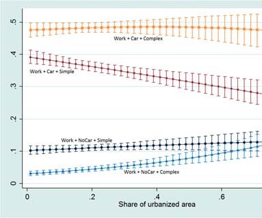
Imprint

Ruhr Economic Papers

Published by
RWI Leibniz-Institut für Wirtschaftsforschung
Hohenzollernstr. 1-3, 45128 Essen, Germany
Ruhr-Universität Bochum (RUB), Department of Economics
Universitätsstr. 150, 44801 Bochum, Germany
Technische Universität Dortmund, Department of Economic and Social Sciences
Vogelpothsweg 87, 44227 Dortmund, Germany
Universität Duisburg-Essen, Department of Economics
Universitätsstr. 12, 45117 Essen, Germany

Editors

Prof. Dr. Thomas K. Bauer
RUB, Department of Economics, Empirical Economics
Phone: +49 (0) 234/3 22 83 41, e-mail: thomas.bauer@rub.de
Prof. Dr. Wolfgang Leininger
Technische Universität Dortmund, Department of Economic and Social Sciences
Economics – Microeconomics
Phone: +49 (0) 231/7 55-3297, e-mail: W.Leininger@tu-dortmund.de
Prof. Dr. Volker Clausen
University of Duisburg-Essen, Department of Economics
International Economics
Phone: +49 (0) 201/1 83-3655, e-mail: vclausen@vwl.uni-due.de
Prof. Dr. Roland Döhrn, Prof. Dr. Manuel Frondel, Prof. Dr. Jochen Kluve
RWI, Phone: +49 (0) 201/81 49 -213, e-mail: presse@rwi-essen.de

Editorial Office

Sabine Weiler
RWI, Phone: +49 (0) 201/81 49 -213, e-mail: sabine.weiler@rwi-essen.de

Ruhr Economic Papers #711

Responsible Editor: Manuel Frondel
All rights reserved. Essen, Germany, 2017
ISSN 1864-4872 (online) – ISBN 978-3-86788-830-1
The working papers published in the Series constitute work in progress circulated to
stimulate discussion and critical comments. Views expressed represent exclusively the
authors’ own opinions and do not necessarily reflect those of the editors.
Ruhr Economic Papers #711

            Michael Simora and Colin Vance

Travel Mode and Tour Complexity:
  The Roles of Fuel Price and Built
                      Environment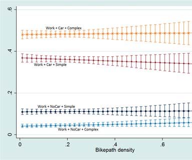
Bibliografische Informationen der Deutschen Nationalbibliothek The Deutsche Nationalbibliothek lists this publication in the Deutsche National bibliografie; detailed bibliographic data are available on the Internet at http://dnb.dnb.de RWI is funded by the Federal Government and the federal state of North Rhine-Westphalia. http://dx.doi.org/10.4419/86788830 ISSN 1864-4872 (online) ISBN 978-3-86788-830-1
Michael Simora and Colin Vance1

Travel Mode and Tour Complexity: The
Roles of Fuel Price and Built Environment

Abstract
Despite steady increases in fuel economy, CO2 emissions from road transportation in
Germany are on the rise, increasing by nearly 4% since 2009. This study analyzes the
impact of different policy levers for bucking this trend, focusing specifically on the role
of fuel prices and features of the built environment. We estimate two multinomial logit
models, one addressing work-related tours and the other non-work related tours. Both
models consider two interrelated dimensions of travel on the extensive margin: mode
choice and tour complexity. We use the model estimates to predict outcome probabilities
for different levels of our policy variables. Our results suggest significant effects of the
built environment – measured by bike path density, urbanization, and proximity to
public transit – in discouraging car use and increasing tour complexity. Fuel prices, by
contrast, appear to have little bearing on these choices.

JEL Classification: D10, R48, R42

Keywords: Activity-based approach; travel mode choice; tour complexity; multinomial
logit; predicted probabilities

September 2017

1 Michael Simora, RWI; Colin Vance, RWI and Jacobs University Bremen. – We thank Manuel Frondel for helpful
commentary and suggestions. Financial support by the Collaborative Research Center “Statistical Modeling of
Nonlinear Dynamic Processes” (SFB 823) of the German Research Foundation (DFG), within Project A3, “Dynamic
Technology Modeling” is gratefully acknowledged.– All correspondence to: Colin Vance, RWI, Hohenzollernstr.
1/3, 45128 Essen, Germany, e-mail: colin.vance@rwi-essen.de
1 Introduction

The transportation sector has emerged as a seemingly intractable obstacle to Ger-
many’s success in reducing CO2 emissions. While the country’s overall CO2 emis-
sions decreased by 27% between 1990 and 2014, emissions in transportation are on
the rise. To buck this trend, legislation was introduced by the European Commis-
sion in 2009 that limits the average emissions of new cars to 130g CO2 /kilometer by
2015 and 95g CO2 /kilometer by 2020 (European Commission, 2009). On its face, the
legislation has been effective: Between 2009 and 2014, the per kilometer CO2 dis-
charge of new cars in Germany decreased by about 14%, from 154.0 to 132.5g CO2
/kilometer (European Environment Agency, 2017). Over the same interval, however,
overall emissions from road transportation in Germany increased by nearly 4%, from
approximately 156 to 162 million tons (Umweltbundesamt, 2016).
  One explanation for these opposing trends is a rising travel demand. Between 2005
and 2014, the mileage of German drivers steadily increased from 875.7 to 935 billion
kilometers (Bundesministerium für Verkehr und digitale Infrastruktur, 2016). Various
factors have contributed to this increase, one being that the real per kilometer costs
of driving decreased due to improved fuel economy and a stagnation in the level of
the ecotax on fuel, which has been set at 0.65 cent per liter for petrol and 0.45 cents
per liter for diesel since 2003. Higher fuel taxes is therefore one of the debated policy
options to decrease emissions, as taxes directly confront motorists with the costs of
driving. Several studies by Frondel and colleagues (Frondel and Vance, 2009, 2014,
2017) using household data from Germany support this tact, estimating fuel price
elasticities for German drivers to be on the order of 60%. Other studies, however, have
found substantially lower responsiveness to the cost of driving, calling into question

                                           4
the effectiveness of fuel taxation as an instrument to reduce emissions (De Borger
et al., 2016; Gillingham et al., 2016; Goodwin et al., 2004; Ritter et al., 2016; Small and
Van Dender, 2007).
These discrepancies raise the question of what policy levers can be availed to dis-
courage automobile dependency. Drawing on data set stemming from 16 years of
individual travel data in Germany, the present paper addresses this issue by present-
ing results from two multinomial logit models, one addressing work-related tours
and the other non-work related tours. Both models consider two interrelated dimen-
sions of travel on the extensive margin: mode choice and tour complexity. Specifi-
cally, the models distinguish four distinct combinations of tour choices according to
whether the car is used and whether the tour is simple or complex, with simple tours
being those without intermediate stops. The model includes a rich array of explana-
tory variables, many of which, including fuel prices, the accessibility of public transit
and bike path density, have immediate relevance for policy, but have rarely been
parametrized using household data. In a second step, we move beyond the standard
focus on the magnitude and significance of the parameter estimates to consider their
implications for predicted outcomes. To this end, we employ a Monte Carlo simula-
tion technique proposed by King et al. (2000) to explore the predictions of the model
and the associated degrees of uncertainty.
Among our main results, we find significant effects of the built environment – mea-
sured by bike path density, urbanization, and proximity to public transit – in discour-
aging car use and increasing tour complexity. Fuel prices, by contrast, appear to have
little bearing on these discrete choices, notwithstanding the high fuel price elastic-
ities that have been estimated for German drivers (Keller and Vance, 2013; Frondel
and Vance, 2017). Taken together, these results suggest that the extension of transit
infrastructure and increased building density hold promise for discouraging car use.
5The paper is organized as follows. In Section 2 we describe the data set, derive
the dependent variable of our model, and introduce the control variables. Section 3
shortly reviews the multinomial logit model. In Section 4 we first show regression
results, followed by the prediction of outcome probabilities. Finally, Section 5 sum-
marizes and concludes.
2 Data
The data is drawn from the German Mobility Panel (MOP, 2015) and covers sixteen
years, spanning 1999 through 2014. Participating individuals are surveyed upwards
of three consecutive years for a period of one week. During this week, they fill out
a drivers’s logbook documenting their travel behavior, including each trip taken, its
purpose, mode, duration, and several other features. In addition, the survey collects
sociodemographic information on the individual and household. A total of 13,500
individuals are observed for an average of 16 tours over the three-year survey period,
yielding a total sample size of approximately 220,000 observations.
2.1 The dependent variable
Following Ben-Akiva and Bowman (1998) as well as Shiftan et al. (2003), who argue
that a tour-based approach is best suited for disaggregate travel demand modeling
when analyzing the influence of built environment, we define our dependent variable
with reference to home-based tours that occur over the five-day work week. While
many studies focus exclusively on work tours (De Palma and Rochat, 1999; Kingham
et al., 2001; Krygsman et al., 2007; Rodrı̀guez and Joo, 2004), we also analyze non-
work related travel, since it considerably contributes to traffic and hence, emissions
(Bhat, 1997). A tour is considered to be work related as soon as at least one trip of the
6tour includes the workplace. Hence, work related tours might incorporate several
non-work related stops. Conversely, we define non-work tours to include any stops
other than work. As work related tours are different from non-work related tours in
the sense that they are non-discretionary and repeatedly undertaken, we model these
tour types separately using two multinomial logit estimators.
Two dimensions are considered in our models. First, we distinguish the travel
mode between car and no car. The latter includes walking, cycling and all modes of
public transit, while the former incorporates all modes of private motorized travel,
including rides as a passenger. Second, we distinguish between simple and complex
tours. Following Strathman and Dueker (1990), we define a tour to be complex if it
consists of more than two trips. For example, a tour from home to work and back is
considered a simple tour. If the individual adds at least one intermediate stop, the
tour becomes complex. Conducting one complex tour instead of several simple ones,
i.e. engaging in trip chaining, is an alternative strategy to reduce car usage.
The two dimensions – mode and complexity – result in four distinct options whose
shares are presented in Table 1. Note that because we exclude individuals who do
not have access to a car as well as individuals who are not working, the presented
shares are not intended to be representative of German travel mode choices. Unsur-
prisingly, complex non-car tours are the least favored option in both cases. It has been
found in previous studies that the complexity of tours is negatively correlated with
the propensity to use non-car options, since stops would need to be in proximity of
each other (Hensher and Reyes, 2000; Krygsman et al., 2007; Strathman and Dueker,
1990).
7Table 1: Different tour options and their sample shares
Option Description Share (in %)
WCS Work + Car + Simple 34.8
WCC Work + Car + Complex 47.0
WNS Work + NoCar + Simple 11.8
WNC Work + NoCar + Complex 6.4
N 123,436
Option Description Share (in %)
NCS NonWork + Car + Simple 46.9
NCC NonWork + Car + Complex 25.6
NNS NonWork + NoCar + Simple 23.7
NNC NonWork + NoCar + Complex 3.8
N 94,488
2.2 The explanatory variables
In assembling the explanatory variables presented in Table 2, we augmented the MOP
with various external data sources to allow investigation of policy-relevant variables
like fuel prices and features of the built environment. Fuel prices are obtained from
the website of Aral, one of Germany’s largest gasoline retailers, which publishes nom-
inal fuel prices by month dating back to 1999. The nominal fuel prices are converted
into real values using a consumer price index from Germany’s Federal Ministry of
Statistics.
Three variables of built environment are used, one of which is derived from
a shapefile of bike paths in Germany gathered from OpenStreetMap.org (Open-
StreetMap, 2017). Using a Geographical Information System (GIS), we intersected
this layer with another shapefile of German counties from the year 2005, at which
time there were 439 counties having an average size of 814 square kilometers. The
resulting intersected shapefile allows us to calculate the total length of bike paths
8Table 2: Descriptive statistics of explanatory variables
Variable Explanation Mean Std.Dev.
female Dummy: 1 if respondent is female 0.526
age Age of respondent 44.98 10.18
fulltime Dummy: 1 if respondent works fulltime 0.656
numemployed Number of employed persons in household 1.73 0.59
kids09 Dummy: 1 if kids between 0 and 9 years 0.198
live in household
kids1017 Dummy: 1 if kids between 10 and 17 years 0.280
live in household
middle Dummy: 1 if middle income household 0.510
(i.e. 1,500 - 3,500 EUR per month)
wealthy Dummy: 1 if wealthy income household 0.423
(i.e. ¿ 3,500 EUR per month)
lackofcars Dummy: 1 if number of cars in household 0.368
is smaller than number of drivers
distancework Distance to work for respondent (in km) 13.03 17.86
rain Dummy: 1 if rain fell on day of travel 0.495
temperature Mean temperature on day of travel 10.59 4.11
petrol Real petrol price in Cents (monthly average) 134.30 14.64
minutes Minutes to walk to nearest bus, tram 5.45 4.62
or train station from respondent’s home
bikepathdens Bikepath density in respondent’s county 0.169 0.161
urbanization Share of urbanized area in respondent’s county 0.195 0.193
1999 Dummy: 1 if year=1999 0.065
2000 Dummy: 1 if year=2000 0.054
2001 Dummy: 1 if year=2001 0.072
2002 Dummy: 1 if year=2002 0.057
2003 Dummy: 1 if year=2003 0.068
2004 Dummy: 1 if year=2004 0.060
2005 Dummy: 1 if year=2005 0.060
2006 Dummy: 1 if year=2006 0.053
2007 Dummy: 1 if year=2007 0.053
2008 Dummy: 1 if year=2008 0.060
2009 Dummy: 1 if year=2009 0.051
2010 Dummy: 1 if year=2010 0.055
2011 Dummy: 1 if year=2011 0.055
2012 Dummy: 1 if year=2012 0.062
2013 Dummy: 1 if year=2013 0.086
2014 Dummy: 1 if year=2014 0.090
in each county. Dividing this by the total area yields a measure of bike path den-
sity. Bhat et al. (2009) find a positive effect of a higher bike path density on opting for
non-motorized travel alternatives, though not distinguishing between work and non-
work related activities. On the contrary, Kingham et al. (2001) as well as Rodrı̀guez
9and Joo (2004) do not detect a significant effect, ascribing their finding to long com-
mute distances precluding an influence of bike paths. However, these two studies
focused solely on work commute, leaving open the possibility that more bike paths
lead to a more frequent use of this mode for recreational, thus non-work related,
travel.
The second metric capturing the built environment measures the extent of urban-
ized area, which was derived in a similar manner using the Corine Land Cover satel-
lite imagery obtained from the website of the European Environmental Agency. The
imagery distinguishes 26 land cover classes in raster format at a resolution of 100 ×
100 meters, and is available for the years 2000 and 2006. We added up the area clas-
sified as artificial surfaces (e.g. urban fabric, industrial and transport units) within
each county to obtain the square kilometers of urbanized area, and divided this by
the total size of the county to obtain the urban share. We assigned the 2000 value
of urban area to the years 1999 through 2005, and the 2006 value to the subsequent
years. Previous studies have found that a higher degree of urbanization fosters tour
complexity (Scheiner and Holz-Rau, 2017; Strathman and Dueker, 1990) as well as
non-motorized travel (Frank et al., 2008; Zhang, 2004).
The remaining variable measuring the built environment is directly recorded in
the MOP and measures the time in minutes to walk from a respondent’s home to
the nearest bus, tram or train station. We expect a closer proximity to decrease the
probability of those options that include the car as a travel mode.
For the variables of the built environment we might face endogeneity issues, as in-
dividuals with less inclination to drive may select into regions with a higher degree
of urbanization and better public transit. While endogeneity cannot be completely
ruled out, we follow the argumentation of Naess (2014) (p. 75), who notes that this
residential self-selection is “unlikely to represent any great source of error ... if tradi-
10tional demographic and socioeconomic variables have already been accounted for.”
Consequently, a suite of sociodemographic control variables is incorporated into our
analysis. These include the individual’s age, gender, and employment status as well
as the proximity of the workplace. They also comprise household level dummy vari-
ables indicating the presence of (young) children, the income level, and whether the
number of licensed drivers is greater than the number of cars. These variables have
been shown to significantly influence travel behavior in previous studies (Bhat, 1997;
Bhat et al., 2009; Hensher and Reyes, 2000; Kuhnimhof et al., 2006; Scheiner and Holz-
Rau, 2017) . Furthermore, we include a measure of the mean temperature on the day
of travel and a dummy indicating whether it rained, as De Palma and Rochat (1999)
found adverse weather conditions to lead to more car usage. The specification is
completed by year dummies to account for changes in travel behavior over time.
3 Methodology
As our dependent variable is nominal without natural ordering, we make use of the
multinomial logit model (MNLM). This section shortly reviews this approach.1
Let J = {1, ..., 4} denote the set of tour options individuals can choose from. As-
suming a standard random utility model (RUM), the utility for individual i from op-
tion j ∈ J is given by:
Uij = Vij + ij . (1)
Here, ij is the unobserved error term and Vij is the observed indirect utility, for which
1 For more details see Long & Freese (2006) for estimation implementation. Furthermore, note that
using a nested logit approach is precluded due to a lack of option specific variables such as travel cost
or time.
11we assume a linear functional form depending on observed characteristics xi :
Vij = β Tj xi . (2)
xi comprises fuel price, the variables measuring built environment, sociodemo-
graphic and household characteristics, and year dummies. β j are the coefficients to
be estimated with superscript T denoting the transposition of a vector. As individual
i chooses option j if its utility is highest from this option, the probability of choosing
option j can be written as:
Pij = Pr (Uij > Uik ) = Pr (ik − ij < Vij − Vik ), ∀k = 1, ..., 4, k = j (3)
If we further assume that the differences in the error terms (ik − ij ) follow a logistic
distribution, we derive the multinomial logit model by rewriting equation 3 as:
β Tj xi
eVij e
Pij = = . (4)
∑4k=1 eVik ∑4k=1 e β k xi
T
From equation 4 it directly follows that the odds between two options just depend on
the parameters of these two options:
Pij
= e ( β j − β k ) xi ,
T
(5)
Pik
which poses a potential shortcoming of the model, known as the independence of
irrelevant alternatives (IIA) assumption. That is, the choice between two alternative
outcomes is unaffected by what other choices are available. While the IIA assumption
is in some contexts restrictive, particularly when relevant options have been omitted
from the definition of the choice set, there are two reasons why it is deemed to be
relatively innocuous for the current application. First, as advocated by McFadden
12(1973) and reiterated by Long and Freese (2006), the multinomal logit model is ap-
propriate when the choice categories are clearly distinct and not substitutes for one
another, a condition that can reasonably be said to apply to the choice between our
different travel options. Second, verification is provided by a Hausman testas well as
a Small-Hsiao test, both support the IIA assumption for our data.
To facilitate the interpretation of selected results from the model, the predicted
probabilities and associated 95% confidence intervals for particular variables of in-
terest are plotted, using a statistical simulation method described in King et al. (2000)
and Tomz et al. (2003). Recognizing that the parameter estimates from a maximum
likelihood model are asymptotically normal, the method uses a sampling procedure
akin to Monte Carlo simulation in which a large number of values – say 1,000 – of
each estimated parameter are drawn from a multivariate normal distribution. Taking
the vector of coefficient estimates from the model as the mean of the normal distri-
bution and the variance-covariance matrix as the variance, the simulated parameter
estimates can be used to calculate predicted values and the associated degree of un-
certainty. In generating the predictions, all explanatory variables except the one of
interest are held constant at their sample mean while the value of the variable under
scrutiny is varied.
4 Results
4.1 Estimates
Table 3 illustrates the effects of our variables of interest on travel behavior for work
related tours while Table 4 presents key results for non-work related tours. Results
for the further controls can be found in Tables X and Y in the Appendix. Note that
during a given day an individual might conduct several tours, which leads to non-
13independent observations. To account for this, we cluster standard errors on the per-
son level.
To ease interpretation, the discussion focuses on odds ratios for the different com-
binations of options. Broadly speaking, an odds ratio bigger than one indicates a
preference for the first of the compared options if the independent variable under
scrutiny increases. Correspondingly, an odds ratio smaller than one indicates a pref-
erence for the second option.
Table 3: Option odds from MNLM for work related tours
WCS/WCC WCS/WNS WCS/WNC WCC/WNS WCC/WNC WNS/WNC
minutes 1.007 1.026** 1.020* 1.019 1.013 0.994
bikepathdens 0.874 0.851** 0.548** 0.974 0.627** 0.644**
urbanization 0.621** 0.457** 0.095** 0.736 0.154** 0.209**
petrol 1.003 0.995 0.983 0.992 0.980 0.988
N 117,038
WCS=Work+Car+Simple; WCC=Work+Car+Complex; WNS=Work+NoCar+Simple; WNC=Work+NoCar+Complex.
** and * denote statistical significance at the 1 % and 5 % level, respectively.
Further controls as well as year dummies are included, though not depicted.
Results reveal that increasing remoteness of the nearest public transit station, mea-
sured by minutes, increases the odds that an individual conducts simple car tours
for work-related travel. The magnitude of the statistically significant estimates for
minutes, however, are relatively modest. For example, each minute increase in the
walking distance to the public transit is seen to increase the odds of using the car for
a simple tour relative to some other mode by just 2.6%. A similar magnitude of 2%
is seen for the comparison of a simple car tour relative to a complex non-car tour.
Thus, a better connection of the respondent’s place of residence to the public transit
network is associated with a somewhat higher propensity to refrain from car usage
for work related tours.
The results further reveal a strong tendency towards non-car travel given a higher
density of bike paths in the respondent’s county of residence. Both simple as well as
14complex tours without the car are preferred over simple car tours. Moreover, there
seems to be a preference of complex tours conducted with non-car modes in areas
with a high density of bike paths. This would suggest that if bike paths were ex-
tended, more individuals would refrain from car usage and chain more trips together
on their work commute. We also find strong effects of the degree of urbanization: Re-
spondents who live in urban areas are less likely to use their car for work-related
tours. Additionally, those individuals more frequently combine trips to complex
tours, especially when traveling without car, which might be explained by a higher
density of places of interest in urban areas.
Last, we see no evidence that the fuel price has an effect on the discrete travel
choices pertaining to work-related tours. We neither find a tendency to refrain from
car usage given high fuel prices, nor a tendency to chain trips together. One expla-
nation for this result is the model’s focus on work travel, which is typically non-
discretionary and hence less responsive to changes in fuel costs.
Table 4: Option odds from MNLM for non-work related tours
NCS/NCC NCS/NNS NCS/NNC NCC/NNS NCC/NNC NNS/NNC
minutes 1.007 1.027** 1.056** 1.019* 1.048** 1.028**
bikepathdens 0.933 0.923** 0.549** 0.989 0.588** 0.594**
urbanization 0.620** 0.391** 0.175** 0.631* 0.282** 0.447**
petrol 0.992 0.996** 1.000 1.004 1.008 1.004
N 76,570
NCS=NonWork+Car+Simple; NCC=NonWork+Car+Complex; NNS=NonWork+NoCar+Simple; NNC=NonWork+NoCar+Complex.
** and * denote statistical significance at the 1 % and 5 % level, respectively.
Further controls as well as year dummies are included, though not depicted.
Table 4 depicts the odds ratios for non-work related tours. Overall, the results
portray a similar pattern as that seen for work related travel. The walking distance to
the nearest transit stop, bike path density, and urban residency all encourage non-car
modes of transportation. In the case of the latter two variables, there is also evidence
for increased complexity of travel. One discrepancy relative to work tours is seen
15for the petrol price, which now registers a significant effect on the odds of car use
for simple tours relative to other modes. Nevertheless, the magnitude of the effect is
relatively small: each cent increase in the petrol price reduces the odds of using the
car by roughly 0.04%.
4.2 Predicted Probabilities
As the proliferation of estimates produced by the MNLM complicates the interpre-
tation of the results, we illustrate the impact of our key variables of interest in this
section by showing predicted probabilities for each travel option using the method of
King et al. (2000).
Results for work related tours are depicted in Figure 1. We focus on the three vari-
ables capturing the built environment. Notwithstanding the statistically significant
odds ratios estimated for these variables, their bearing on the predicted probabilities
is in many cases marginal. This is especially evident for the case of bike path density,
where the curves corresponding to each choice combination are seen to be relatively
flat.
Across the graphs, the highest probability, at about 0.47, is seen for the option com-
bining car travel with complex tours. Again, however, the flat trajectory of the curve
suggests that this is also the option that is least responsive to changes in the explana-
tory variables. The next most probable option is given by the combination of car use
with simple tours. The probability of this option is seen to increase with increasing
minutes to the nearest transit stop and to decrease with a higher share of urbanized
area in the county of residence.
Non-car modes for work commute are the two least probable options. For complex
tours, the probability increases markedly with a higher share of urbanized area, more
than doubling from a low of about 0.05 to a high of 0.13 when the urban share reaches
16Figure 1: Predicted probabilities for work related tour options depending on variables
of the built environment
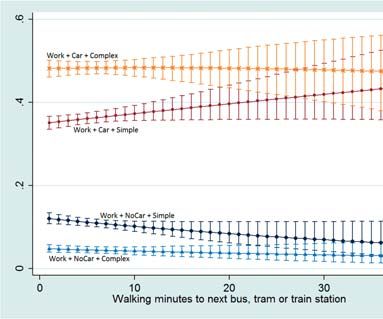
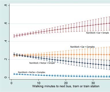
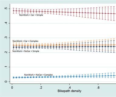
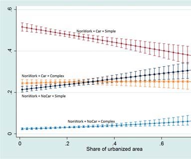
17Figure 2: Predicted probabilities for non-work related tour options depending on
variables of the built environment
180.8. Likewise, simple non-car tours respond strongly to public transit proximity, being
more likely when the station is nearby.
Figure 2 depicts predicted probabilities for non-work related tours. The most prob-
able option is now the one combining car travel with simple tours, indicating that trip
chaining is less likely when work stops are not part of the tour. This option appears
relatively responsive to changes in walking minutes to public transit and the share of
urban area, increasing with the former and decreasing with the latter. Likewise, non-
car simple tours are responsive to these two variables, in this case decreasing with the
former and increasing with the latter. It is also notable that the probability of non-car
simple tours, which ranges between nearly 0.2 and 0.3, is roughly twice that of the
corresponding probability for work-related travel.
Regarding bike path density, we again observe discrepancies between the statisti-
cally significant regression results and a relatively flat pattern of the predicted proba-
bilities (middle chart). Taken together, we conclude that an increase in bike paths has
little bearing on travel probabilities relating to work and non-work purposes.
5 Conclusion
Using a large data set stemming from 16 years of a household travel diary panel,
this paper has analyzed the roles of the fuel price and the built environment on work
and non-work related tours. To this end, we first estimated a multinomial logit model
that considered mode and the complexity of travel, two decisions that interrelate with
each other and thus should be scrutinized jointly (Bhat, 1997; Feng et al., 2013; Krygs-
man et al., 2007). In a second step we estimated outcome probabilities for different
levels of our policy levers.
Several findings emerge. First, for work related tours, we find no evidence for an
effect of fuel prices on the discrete choice pertaining to mode and tour complexity.
19This result may be partially explained by the fact that such tours are for the most
part non-discretionary and hence less likely to be subject to changes in fuel costs. For
non-work travel, we find slight evidence for an effect of the fuel price, decreasing the
odds that the car is used for simple tours. Overall there seems to be limited response
of individuals to fuel price changes with respect to discrete work-related travel de-
cisions. This may owe to the possibility that individuals react via investing in more
fuel efficient vehicles if fuel prices continue to increase (Bhat et al., 2009; Feng et al.,
2013; Goodwin et al., 2004).
Regarding features of the built environment, we find a statistically significant
but modest effect of a higher bike path density in the respondent’s county. Al-
though regression results suggest a tendency towards non-car travel with more bike
paths being available, the predicted probabilities reveal little decrease in car usage.
Thus, making bike use more practicable seems to foster only a muted effect on non-
motorized travel. This might be ascribed to long commute distances or inconve-
niences in e.g. shopping with bike.
By contrast, we observe a significant impact of public transit proximity on dis-
couraging car use for simple tours. This effect is more pronounced for non-work
related travel than for work commute. In line with previous studies, we conclude
that extending public transit is the most promising approach to discourage car use
(De Palma and Rochat, 1999; Frank et al., 2008; Gärling and Schuitema, 2007; King-
ham et al., 2001). Results from Weis et al. (2010) moreover suggest that price elastic-
ities for public transit are higher than for car use, especially for leisure trips. Conse-
quently, subsidizing public transit should lead to stronger reactions than increasing
fuel prices. If public transit can compete better with car usage in terms of comfort
and price, individuals might switch.
However, certain barriers remain. For commuters, the distance to work still is an
20important obstacle for refraining from car usage (Gorham et al., 2002; Kingham et al.,
2001). Furthermore, for some users driving their own car is still a matter of social
status, while there is a stigma associated with the use of public transit (Aarts and
Dijksterhuis, 2000; Gärling and Schuitema, 2007; Gorham et al., 2002; Jensen, 1999).
Nevertheless, the evidence in this and other studies (Bamberg et al., 2003; Kingham
et al., 2001) shows that individuals react to infrastructure improvements making pub-
lic transit more convenient. In particular, young adults, who have not built up strong
travel habits yet, have been found to be willing to change to other modes of transport
than car (Kuhnimhof et al., 2012).
Future research should address the impact of neighborhood compacts as well as
of information and feedback about the environmental friendliness of travel habits as
these have been found to change travel behavior in other studies (Rose and Ampt,
2001; Taylor and Ampt, 2003).
21References
Aarts, H., Dijksterhuis, A., 2000. The automatic activation of goal-directed behaviour:
The case of travel habit. Journal of Environmental Psychology 20 (1), 75–82.
Bamberg, S., Ajzen, I., Schmidt, P., 2003. Choice of travel mode in the theory of
planned behavior: The roles of past behavior, habit, and reasoned action. Basic and
Applied Social Psychology 25 (3), 175–187.
Ben-Akiva, M. E., Bowman, J. L., 1998. Activity based travel demand model systems.
In: Equilibrium and advanced transportation modelling. Springer, pp. 27–46.
Bhat, C. R., 1997. Work travel mode choice and number of non-work commute stops.
Transportation Research Part B: Methodological 31 (1), 41–54.
Bhat, C. R., Sen, S., Eluru, N., 2009. The impact of demographics, built environment
attributes, vehicle characteristics, and gasoline prices on household vehicle hold-
ings and use. Transportation Research Part B: Methodological 43 (1), 1–18.
Bundesministerium für Verkehr und digitale Infrastruktur, Apr. 2016. Verkehr in
Zahlen 2016/2017. Tech. Rep. 2, Berlin.
URL www.eea.europa.eu/highlights/reported-co2-emissions-from-new
De Borger, B., Mulalic, I., Rouwendal, J., 2016. Measuring the rebound effect with mi-
cro data: A first difference approach. Journal of Environmental Economics and Man-
agement 79, 1–17.
De Palma, A., Rochat, D., 1999. Understanding individual travel decisions: Results
from a commuters survey in geneva. Transportation 26 (3), 263–281.
European Commission, Apr. 2009. Regulation No 443/2009 of the European Parlia-
ment and of the Council of 23 April 2009 setting emission performance standards
22for new passenger cars as part of the Community’s integrated approach to reduce
CO2 emissions from light-duty vehicles. Tech. Rep. 2, Brussels.
URL http://www.ncbi.nlm.nih.gov/pubmed/22373637
European Environment Agency, Apr. 2017. Reported CO2 emissions from new cars
continue to fall. . Tech. Rep. 2, Copenhagen.
URL www.eea.europa.eu/highlights/reported-co2-emissions-from-new
Feng, Y., Fullerton, D., Gan, L., 2013. Vehicle choices, miles driven, and pollution
policies. Journal of Regulatory Economics 44 (1), 4–29.
Frank, L., Bradley, M., Kavage, S., Chapman, J., Lawton, T. K., 2008. Urban form,
travel time, and cost relationships with tour complexity and mode choice. Trans-
portation 35 (1), 37–54.
Frondel, M., Vance, C., 2009. Do high oil prices matter? Evidence on the mobility
behavior of german households. Environmental and Resource Economics 43 (1), 81–
94.
Frondel, M., Vance, C., 2014. More pain at the diesel pump? An econometric compar-
ison of diesel and petrol price elasticities. Journal of Transport Economics and Policy
48 (3), 449–463.
Frondel, M., Vance, C., 2017. Drivers’ response to fuel taxes and efficiency standards:
Evidence from Germany. Transportation, 1–13.
Gärling, T., Schuitema, G., 2007. Travel demand management targeting reduced pri-
vate car use: Effectiveness, public acceptability and political feasibility. Journal of
Social Issues 63 (1), 139–153.
Gillingham, K., Rapson, D., Wagner, G., 2016. The rebound effect and energy effi-
ciency policy. Review of Environmental Economics and Policy 10 (1), 68–88.
23Goodwin, P., Dargay, J., Hanly, M., 2004. Elasticities of road traffic and fuel consump-
tion with respect to price and income: A review. Transport Reviews 24 (3), 275–292.
Gorham, R., Black, W., Nijkamp, P., 2002. Car dependence as a social problem. Social
Change and Sustainable Transport, 107–115.
Hensher, D. A., Reyes, A. J., 2000. Trip chaining as a barrier to the propensity to use
public transport. Transportation 27 (4), 341–361.
Jensen, M., 1999. Passion and heart in transport—a sociological analysis on transport
behaviour. Transport Policy 6 (1), 19–33.
Keller, R., Vance, C., 2013. Landscape pattern and car use: Linking household data
with satellite imagery. Journal of Transport Geography 33, 250–257.
King, G., Tomz, M., Wittenberg, J., 2000. Making the most of statistical analyses: Im-
proving interpretation and presentation. American Journal of Political Science 44 (2),
347–361.
Kingham, S., Dickinson, J., Copsey, S., 2001. Travelling to work: Will people move out
of their cars. Transport Policy 8 (2), 151–160.
Krygsman, S., Arentze, T., Timmermans, H., 2007. Capturing tour mode and activity
choice interdependencies: A co-evolutionary logit modelling approach. Transporta-
tion Research Part A: Policy and Practice 41 (10), 913–933.
Kuhnimhof, T., Buehler, R., Wirtz, M., Kalinowska, D., 2012. Travel trends among
young adults in germany: Increasing multimodality and declining car use for men.
Journal of Transport Geography 24, 443–450.
Kuhnimhof, T., Chlond, B., von der Ruhren, S., 2006. Users of transport modes
and multimodal travel behavior steps toward understanding travelers’ options
24and choices. Transportation Research Record: Journal of the Transportation Research
Board (1985), 40–48.
Long, J. S., Freese, J., 2006. Regression Models for Categorical Dependent Variables Using
Stata. Stata press.
McFadden, D., 1973. Conditional logit analzsis of qualitative choice behvaior. Aca-
demic Press.
MOP, 2015. MOP: The German Mobility Panel. http://mobilitaetspanel.ifv.
uni-karlsruhe.de/de/studie/index.html,accessedApril2016.
Naess, P., 2014. Tempest in a teapot: The exaggerated problem of transport-related
residential self-selection as a source of error in empirical studies. Journal of Transport
and Land Use 7 (3), 57–79.
OpenStreetMap, 2017. OpenStreetMap - Deutschland. https://www.openstreetmap.
de/,accessedJune2016.
Ritter, N., Schmidt, C. M., Vance, C., 2016. Short-run fuel price responses: At the
pump and on the road. Energy Economics 58, 67–76.
Rodrı̀guez, D. A., Joo, J., 2004. The relationship between non-motorized mode choice
and the local physical environment. Transportation Research Part D: Transport and
Environment 9 (2), 151–173.
Rose, G., Ampt, E., 2001. Travel blending: An Australian travel awareness initiative.
Transportation Research Part D: Transport and Environment 6 (2), 95–110.
Scheiner, J., Holz-Rau, C., 2017. Women’s complex daily lives: A gendered look at trip
chaining and activity pattern entropy in Germany. Transportation 44 (1), 117–138.
25Shiftan, Y., Ben-Akiva, M., Proussaloglou, K., de Jong, G., Popuri, Y., Kasturirangan,
K., Bekhor, S., 2003. Activity-based modeling as a tool for better understanding
travel behaviour. In: 10th International Conference on Travel Behaviour Research. pp.
10–15.
Small, K. A., Van Dender, K., 2007. Long run trends in transport demand, fuel price
elasticities and implications of the oil outlook for transport policy. OECD Publish-
ing.
Strathman, J. G., Dueker, K. J., 1990. Understanding trip chaining. Special Reports on
Trip and Vehicle Attributes, 1–1.
Taylor, M. A., Ampt, E. S., 2003. Travelling smarter down under: policies for volun-
tary travel behaviour change in Australia. Transport Policy 10 (3), 165–177.
Tomz, M., Wittenberg, J., King, G., 2003. CLARIFY: Software for Interpreting Statisti-
cal Results. Version 2.1. Stanford University, University of Wisconsin, and Harvard
University. January.
Umweltbundesamt, Apr. 2016. Climate Change 24/2016. Submission under the
United Nations Framework Convention on Climate Change and the Kyoto Pro-
tocol 2016. National Inventory Report for the German Greenhouse Gas Inventory
1990-2014. Tech. Rep. 2, Dessau.
URL www.eea.europa.eu/highlights/reported-co2-emissions-from-new
Weis, C., Axhausen, K., Schlich, R., Zbinden, R., 2010. Models of mode choice and mo-
bility tool ownership beyond 2008 fuel prices. Transportation Research Record: Journal
of the Transportation Research Board (2157), 86–94.
Zhang, M., 2004. The role of land use in travel mode choice: Evidence from Boston
and Hong Kong. Journal of the American Planning Association 70 (3), 344–360.
26Appendix
Table A1: Option odds from MNLM for work related tours: Full Model
WCS/WCC WCS/WNS WCS/WNC WCC/WNS WCC/WNC WNS/WNC
minutes 1.007 1.026** 1.020* 1.019 1.013 0.994
bikepathdens 0.874 0.851** 0.548** 0.974 0.627** 0.644**
urbanization 0.621** 0.457** 0.095** 0.736 0.154** 0.209**
petrol 1.003 0.995 0.983 0.992 0.980 0.988
female 0.744** 0.820 0.549** 1.102 0.738** 0.670
age 1.008** 0.997 1.013 0.989 1.005 1.016
fulltime 0.907 1.189** 0.859 1.311** 0.947 0.722**
numemployed 1.173** 1.205* 1.464** 1.028 1.248** 1.215*
kids09 0.735** 0.913 0.732* 1.242* 0.997 0.803
kids1017 1.139* 1.112 1.378** 0.976 1.210 1.239
middle 0.778** 1.019 0.949 1.310* 1.220 0.931
wealthy 0.592** 0.983 0.637** 1.661** 1.075 0.647*
lackofcars 1.189** 0.347** 0.358** 0.292** 0.301** 1.031
distancework 1.007** 1.021 1.058 1.013 1.050 1.036
rain 0.989 0.984 1.072 0.995 1.085 1.090
temperature 0.998 1.006 1.011 1.008 1.012 1.004
N 117,038
WCS=Work+Car+Simple; WCC=Work+Car+Complex; WNS=Work+NoCar+Simple; WNC=Work+NoCar+Complex.
** and * denote statistical significance at the 1 % and 5 % level, respectively.
Year dummies are included, though not depicted.
27Table A2: Option odds from MNLM for non-work related tours: Full Model
NCS/NCC NCS/NNS NCS/NNC NCC/NNS NCC/NNC NNS/NNC
minutes 1.007 1.027** 1.056** 1.019* 1.048** 1.028**
bikepathdens 0.933 0.923** 0.549** 0.989 0.588** 0.594**
urbanization 0.620** 0.391** 0.175** 0.631* 0.282** 0.447**
petrol 0.992 0.996** 1.000 1.004 1.008 1.004
female 0.890* 0.902 0.620** 1.013 0.696** 0.687
age 1.016** 0.998 1.016 0.982 1.000 1.018
fulltime 1.301** 1.101** 1.330* 0.847** 1.022 1.208
numemployed 1.097* 1.090 1.077** 0.994 0.982 0.989
kids09 0.800** 0.797** 0.597** 0.996 0.746 0.749*
kids1017 1.269** 1.376** 1.761** 1.084 1.388** 1.280*
middle 1.087 1.064 1.592** 0.978 1.464* 1.497**
wealthy 0.956 1.281* 1.405** 1.341* 1.470* 1.096
lackofcars 1.051 0.741** 0.568** 0.705** 0.540** 0.766
distancework 0.999 1.002 1.004 1.003 1.005 1.002
rain 0.938 1.078 1.087 1.149 1.159 1.009
temperature 1.002 0.994 1.000 0.992 0.997 1.005
N 76,570
NCS=NonWork+Car+Simple; NCC=NonWork+Car+Complex; NNS=NonWork+NoCar+Simple; NNC=NonWork+NoCar+Complex.
** and * denote statistical significance at the 1 % and 5 % level, respectively.
Year dummies are included, though not depicted.
28You can also read